
Reliability Analysis of Distribution Systems with Photovoltaic Generation Using a Power Flow Simulator and a Parallel Monte Carlo Approach

Abstract
:1. Introduction
2. Procedure for Distribution Reliability Calculation
2.1. Description of the Procedure
- Run the test system during one year using time-based power flow simulation and a constant time step (e.g., 1 h). This run, known in this work as base case, provides basic information (e.g., energy values) that will be used for later calculations. Depending on the system under study, the simulation can be carried out with or without distributed generation.
- Estimate in advance all the random values related to the faults/failures to be simulated (location/component, time of occurrence, duration, type) for one year.
- Run the test system again but considering now the possibility of fault and/or equipment failure. Regardless of the location, type and duration of the fault/failure, a protective device will always operate. Reliability indices are updated once this sequence of events is finished.
- Repeat the procedure from Step 2 as many times as required to obtain the information needed for estimating reliability indices.
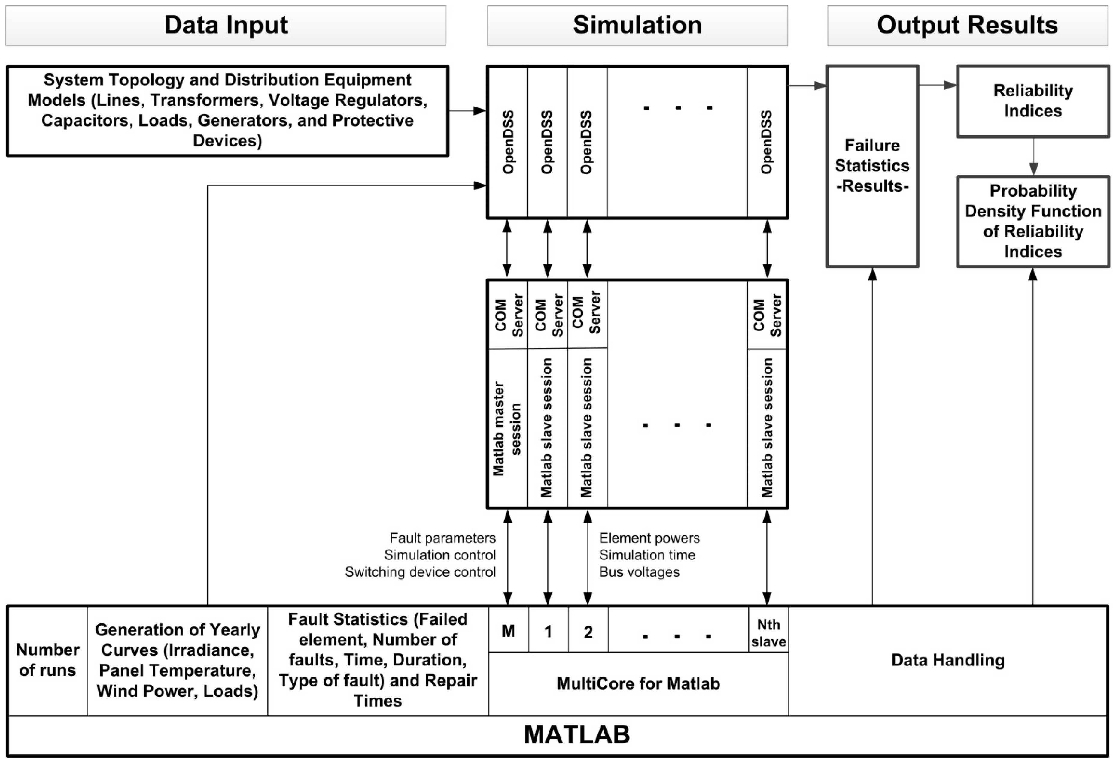
2.2. Implementation of the Procedure
3. Test System
- Rated voltage: 4.16 kV.
- Rated power of substation transformer: 10,000 kVA.
- Rated PV generation power (peak value): 1800 kW.
- Number of load nodes: 107.
- Overall number of customers: 713.
- Average rated power per MV load node: 74.77 kVA.
- Overall line length: 52.1 km.
4. Reliability Model
4.1. Modelling Approach
4.2. Parameters for Reliability Assessment
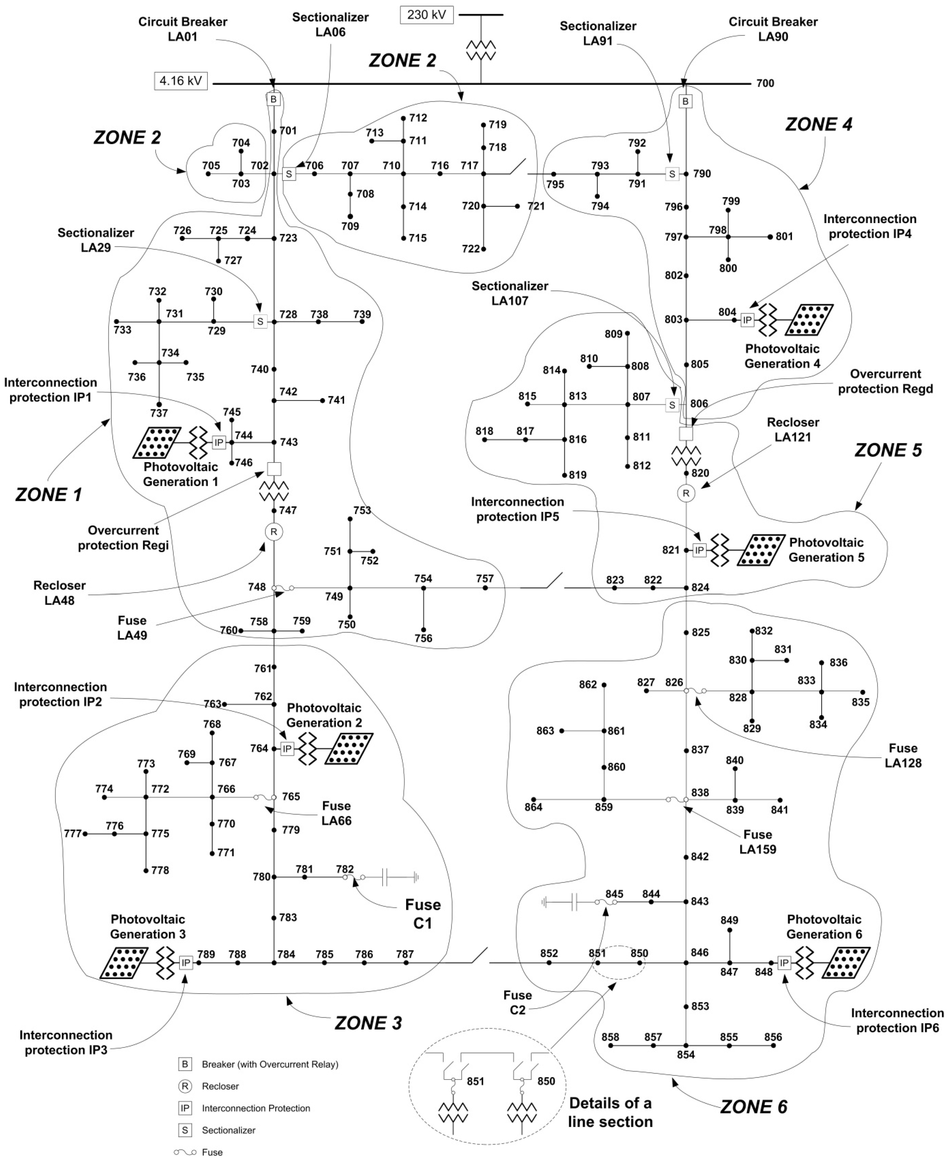
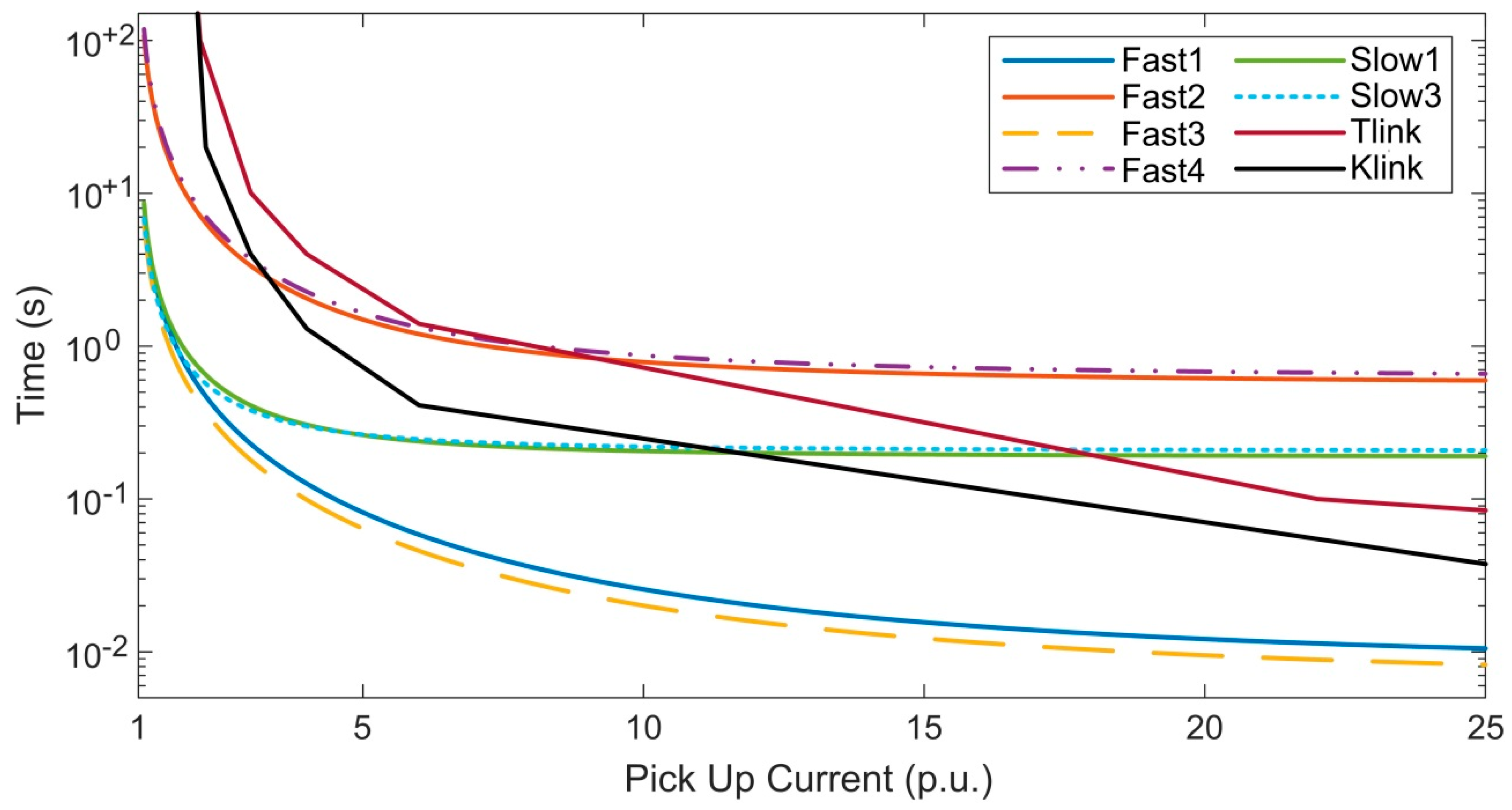
- Protective Devices: Figure 2 shows the type and location of the protective devices installed in the test system. The characteristic time-current curves are similar to those used in [5]; they are shown in Figure 3. The interconnection protection of each generator has over-/undervoltage and overcurrent protection. If a generator is disconnected after a fault, it will be reconnected when normal voltage values at the point of common coupling (PCC) are confirmed (>0.9 pu). On the other hand, it is assumed that PV generators do not suffer any damage during a fault and can be put back in operation as soon as possible. Table 1 provides some information about the devices installed to protect feeders and the interconnection protection of PV plants. Take into account that: (i) reclosers can perform up to three opening operations, two of which use the faster characteristic; (ii) fuses are coordinated using a fuse saving scheme; (iii) sectionalizers count up to two operations before performing an opening action. In all devices with automatic reclosing capabilities, the assumed dead times are 10 and 20 seconds. Except the sectionalizer model, which is a custom-made model, the models used to represent protective devices are those available in OpenDSS.
- Failure Statistics: A fault/failure is fully defined by specifying the faulted component (line, voltage regulator, or capacitor bank), the occurrence time, the duration, and the fault type. Table 2 shows the statistics assumed for this study. Except for PV generators, the explanations about the way in which this information is applied were given in [5]. The reliability model of a PV plant is rather complex; see, for instance, [4,28,29,30]. Implementing and applying a very detailed model is out of the scope of this study; instead a simplified reliability model is used. All PV generators consist of one or more 100 kW modules, being each module characterized by the same failure rate and repair time. Therefore, the parameters to be defined for reliability assessment of a PV generation unit are the rated power (i.e., the number of 100 kW modules), the failure rate and the mean repair time. A PV plant can totally reduce the power it injects into the system when either the interconnection transformer or all modules fail; the reduction of injected power will be partial when not all PV modules fail. The reliability parameters for the interconnection transformer are those used for any other distribution transformer, while the parameters for characterizing the PV modules are those shown in Table 2. The number of PV module failures in a year will be randomly generated using the failure rate shown in Table 2 and following a Poisson distribution. For every failure the number of failed modules must be determined using also a Poisson distribution. The average repair time is the result of multiplying the number of failed modules by the mean repair time; the actual repair time will be randomly calculated using an exponential distribution.
5. An Illustrative Case Study
5.1. Aim of the Case Study
5.2. Characteristics of the Case Study
- Location: Line section LA93, between load nodes 791 and 793.
- Time of occurrence: 2750 h.
- Type of fault: Phase-to-phase (two-phase fault).
- Faulted phases: A and B.
- Duration: Sustained.
- Scenario: Disconnection and repair of the failed element with load transfer between feeders.
5.3. Sequence of Events
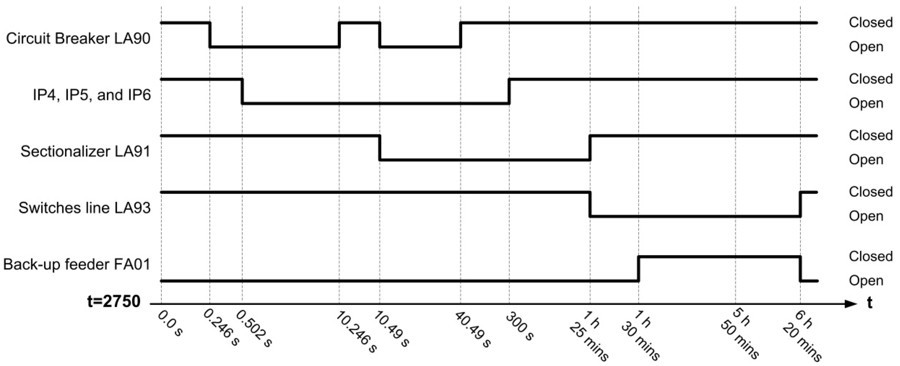
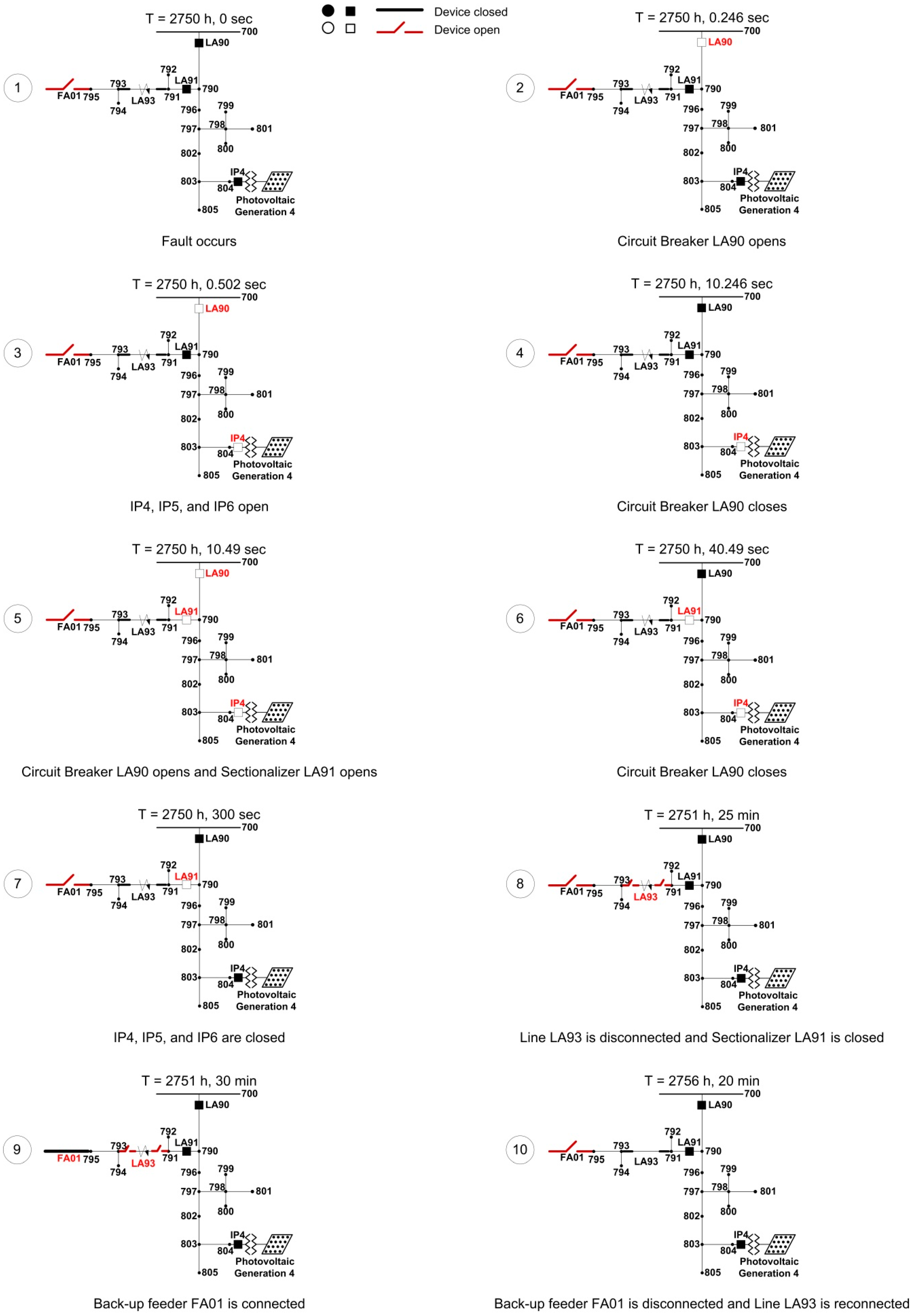
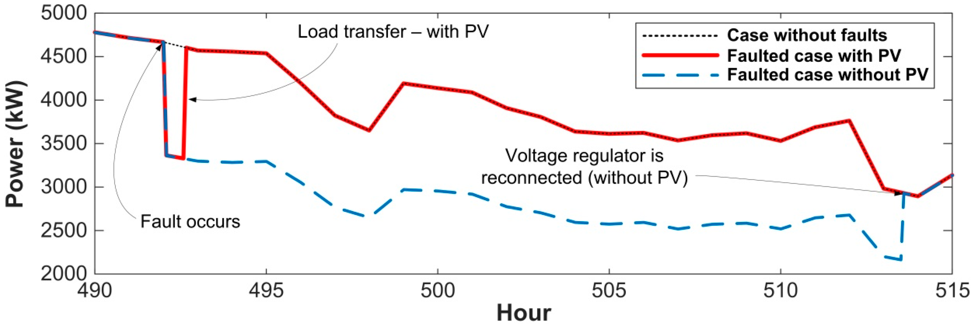
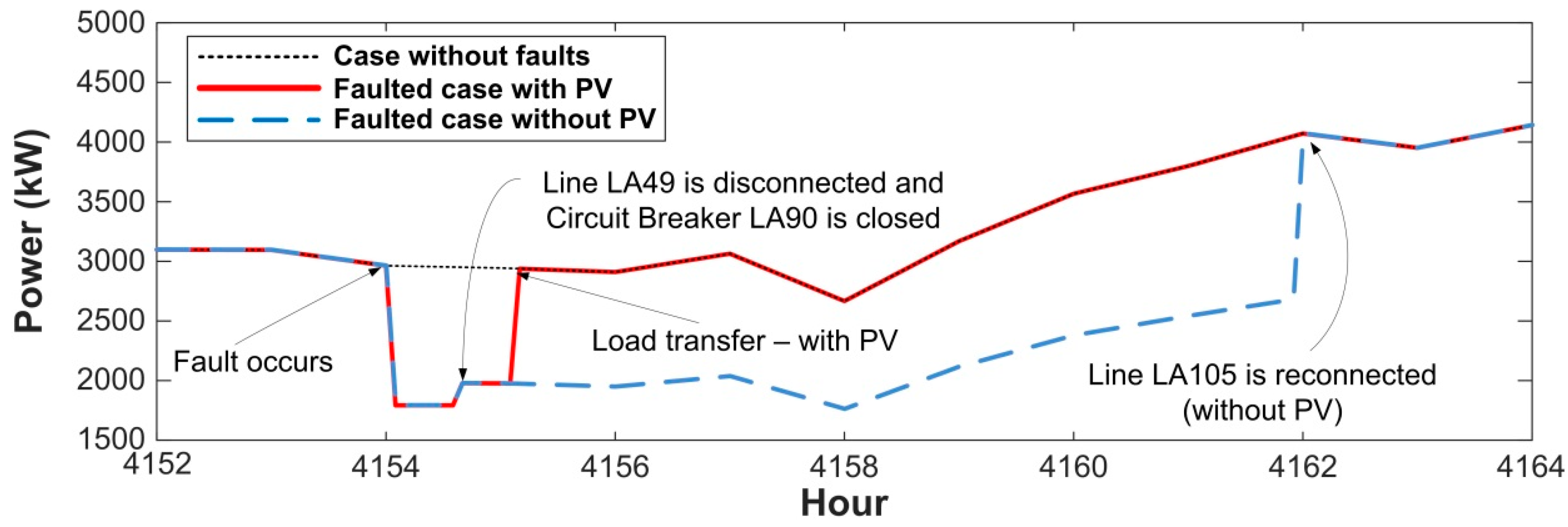
- Figure 4 shows how the configuration of the system changes during the sequence of events caused by the analyzed fault and the status of the various protective devices and switches/disconnectors involved in this case. Remember that, once the fault occurs, the first steps in the sequence of events are caused by the design and settings of the protection system, while the last steps will depend on the performance of the maintenance crew.
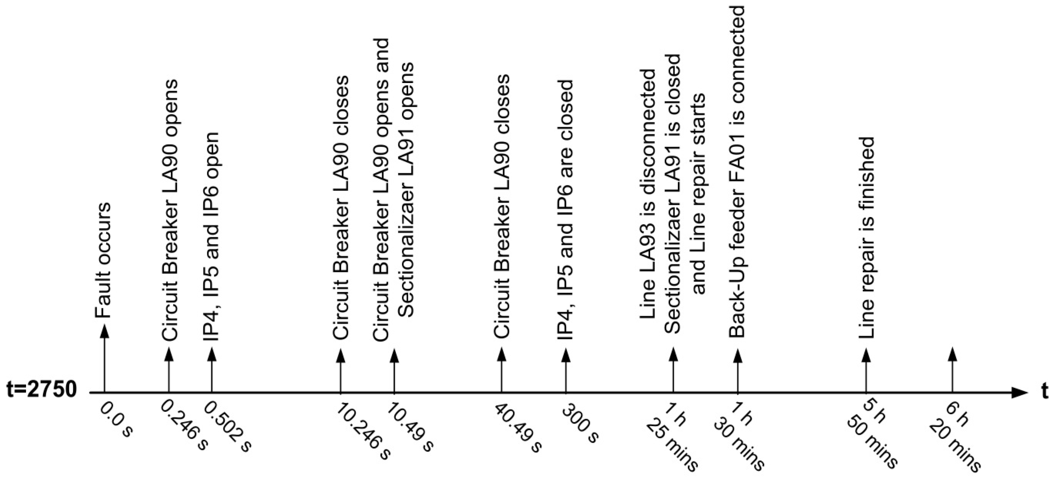
- Figure 5 provides a sequence of events with the time of occurrence of each event. As mentioned above, some of the values required to obtain this sequence are derived from the operation of the protective devices and are of deterministic nature, while others due to the performance of the maintenance crew are of random nature and generated according to the estimated probability distributions, see Section 6.
- Figure 6 shows a diagram with the status (e.g., opened/closed) of the protective devices and switches/disconnectors involved in this case.
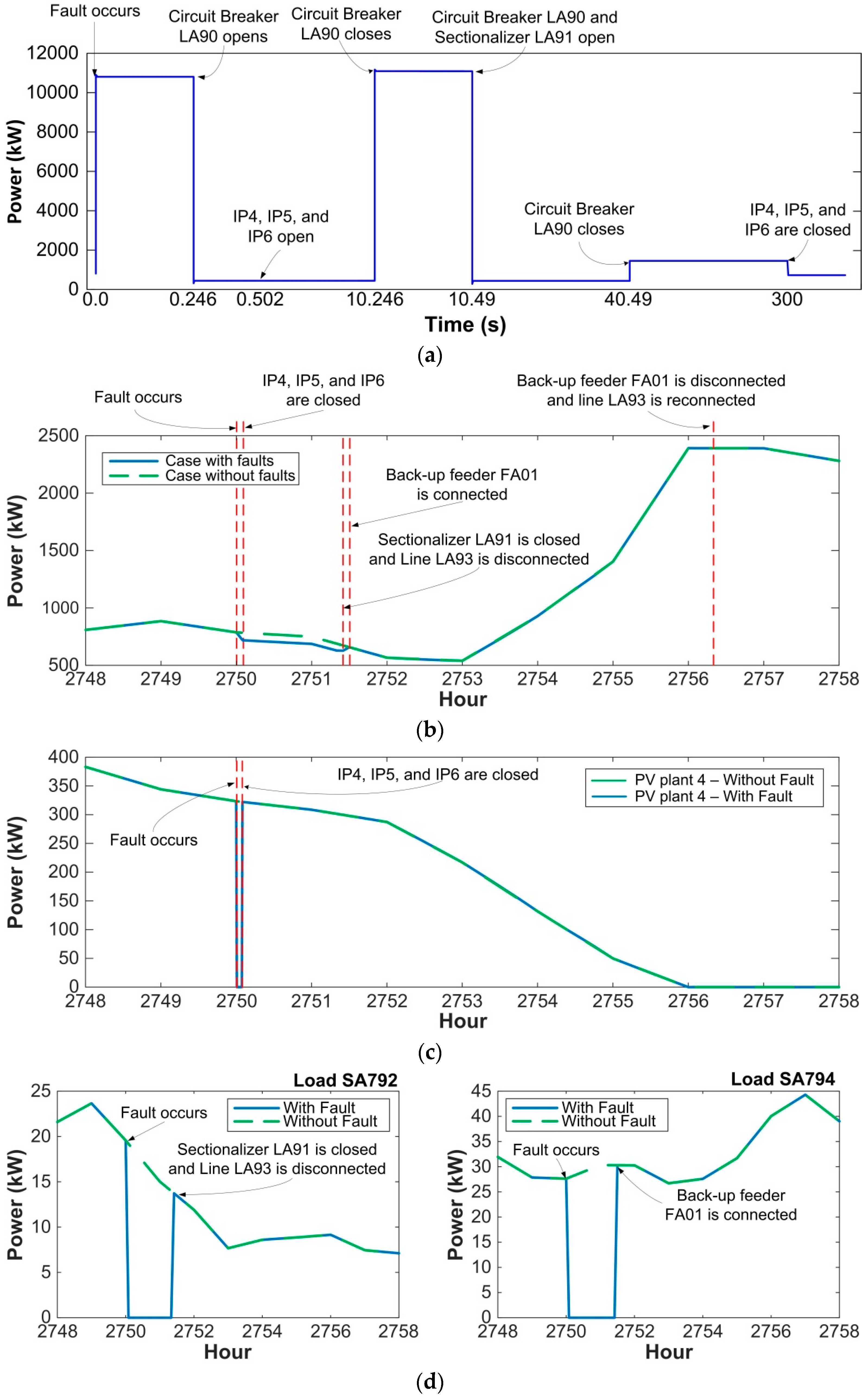
5.4. Simulation Results
6. Studies and Results
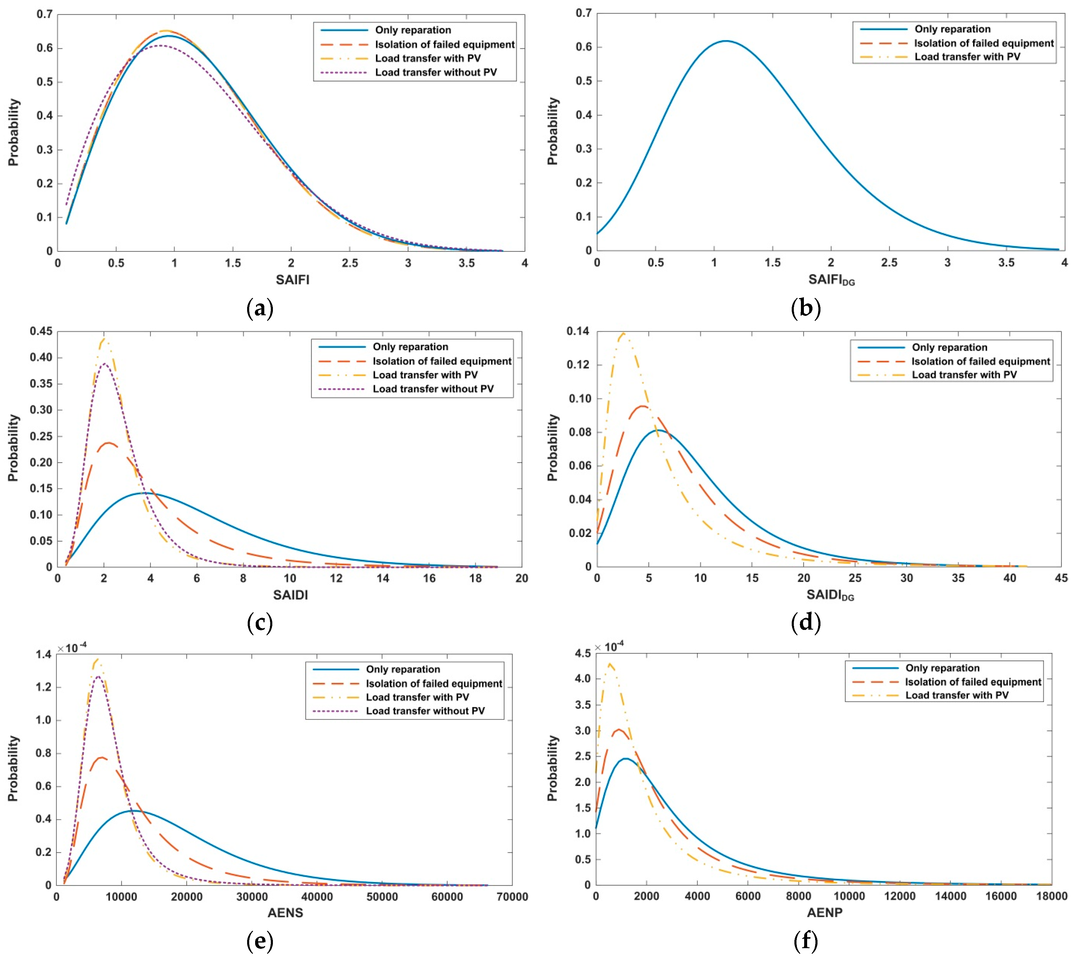
6.1. Reliability Studies
- Only protective devices operate; that is, a protection device locks out after a permanent fault, and service is not restored before the faulted component is repaired.
- Switching operations aimed at isolating the faulted section are performed; this may restore service only to load nodes upstream the failed component.
- System reconfiguration may be used by means of transfer switches between feeders to restore service to some load nodes downstream the faulted section, depending on the system design.
6.2. Some Remarks
- Network reconfiguration and surplus in PV generation can cause reverse power flow through voltage regulators. Reverse power flow can interfere with voltage regulator control and cause unacceptable operating conditions; therefore, voltage regulator control will be disabled during reverse power flow.
- A fault in a line section close to the substation will cause a voltage dip at the nodes of the adjacent feeder, and this could cause the operation of the undervoltage protection of PV generators. Protective devices have been coordinated to avoid these consequences; that is, the overcurrent relay installed to protect the faulted feeder will be faster that the undervoltage protection of PV generators connected to the adjacent feeder.
- Load transfer will be carried out only when normal operating conditions are ensured. That is, when load transfer is considered, the procedure will be as follows: (1) check for availability of back-up feeder; (2) if there is an available back-up feeder, load is transferred; (3) during the simulation, voltages at load points and phase currents through lines and voltage regulators are monitored; (4) when the simulation is finished, the procedure checks for the technical restrictions (all load point voltages are above 0.9 pu; phase current through distribution lines and voltage regulators do not exceed 110% of nominal rating); (5) if one of the previous restrictions is not satisfied the procedure will deem the operation not successful and repeat the simulation without considering load transfer.
- Some special situations have to be considered; one of these situations can occur when load transfer is possible and two maintenance crews are involved: one will take care of the repair and associated operations (e.g., isolation of the failed component), the other one will take care of the transfer maneuver. Both actions are considered independent from each other, and the moments at which the repair of the failed component will finish and the transfer maneuver will be made are randomly estimated. As a consequence of these calculations, the transfer maneuver should be made prior to the moment at which the other crew would finish the repair; if the time interval between the two moments is shorter than 15 min then the transfer operation is not carried out to avoid that an additional maneuver had to be made short after the failed component was repaired.
- A different situation can occur with the previous scenario if some remote control and small values are assumed for some switching times. Remember that back-up feeder connection time is randomly generated and follows an exponential distribution. Two cases have been considered:
- -
- Back-up feeder connection time is shorter than the time needed to disconnect the failed element and close the operated protective device: in this case the procedure will perform both actions simultaneously, using the longer time for both actions.
- -
- Back-up feeder connection time is longer than the time needed to disconnect the failed element and close the operated protective device: for this condition the procedure will perform both actions independently at their specified times.
- If a one-phase fault occurs on a distribution line protected by a fuse, two cases can be considered:
- -
- Phase voltages at LV load points are above 0.9 pu: the repair will be carried out in a normal manner; loads will not experience any interruption.
- -
- Phase voltages at LV load points are below 0.9 pu: the healthy phases will then be opened, isolating all elements downstream from the operated fuse.
If a two-phase fault occurs on a distribution line protected by a fuse, the remaining phase must be opened to disconnect all voltage sources from the failed zone.
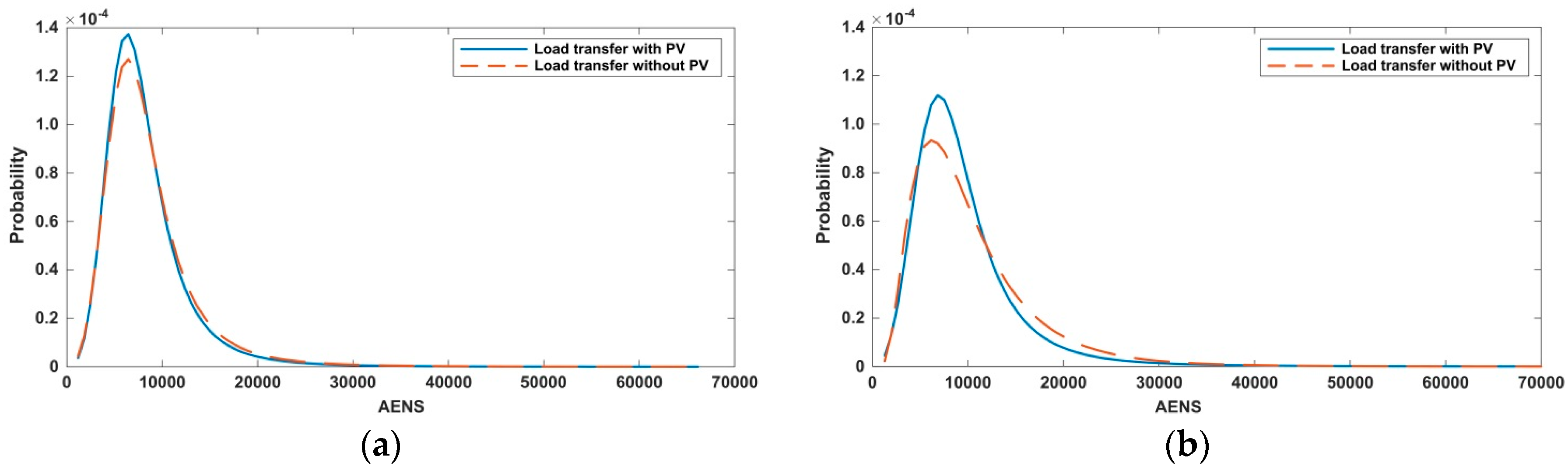
6.3. Reliability Indices
- System Average Interruption Frequency Index for DG (SAIFIDG):
- System Average Interruption Duration Index for DG (SAIDIDG):where k is the number of sustained interruptions in the distribution system corresponding to a given year, PGi is the number of rated kWs of PV generation disconnected from the system during an interruption in the system, PGT is the total rated generation, measured in kW, and Hi is the duration of the disconnection for the PV generation affected by the interruption.
6.4. Simulation Results
6.5. Simulation Time
7. Impact of Distributed Generation on Distribution System Reliability
8. Discussion
9. Conclusions
Author Contributions
Conflicts of Interest
References
- Ackerman, T.; Andersson, G.; Söder, L. Distributed generation: A definition. Electr. Power Syst. Res. 2001, 57, 195–204. [Google Scholar] [CrossRef]
- Lee Willis, H.; Scott, W.G. Distributed Power Generation. Planning and Evaluation; CRC Press: Boca Raton, FL, USA, 2000. [Google Scholar]
- De Leon, F.; Salcedo, R.; Ran, X.; Martinez-Velasco, J.A. Time-Domain Analysis of the Smart Grid Technologies: Possibilities and Challenges. In Transient Analysis of Power Systems: Solution Techniques, Tools and Applications; Martinez-Velasco, J.A., Ed.; John Wiley: Chichester, UK, 2015. [Google Scholar]
- Borges, C.L.T. An overview of reliability models and methods for distribution systems with renewable energy distributed generation. Renew. Sustain. Energy Rev. 2012, 16, 4008–4015. [Google Scholar] [CrossRef]
- Martinez-Velasco, J.A.; Guerra, G. Parallel Monte Carlo approach for distribution reliability assessment. IET Gener. Transm. Distrib. 2014, 8, 1810–1819. [Google Scholar] [CrossRef]
- Dugan, R.C. Reference Guide. The Open Distribution System Simulator (OpenDSS); Electric Power Research Institute (EPRI): Palo Alto, CA, USA, 2012. [Google Scholar]
- Dugan, R.C.; McDermott, T.E. An open source platform for collaborating on smart grid research. In Proceedings of the IEEE Power & Energy Society General Meeting, Detroit, MI, USA, 24–29 July 2011.
- Brown, R.E. Electric Power Distribution Reliability, 2nd ed.; CRC Press: Boca Raton, FL, USA, 2009. [Google Scholar]
- Chowdhury, A.A.; Koval, D.O. Power Distribution System Reliability. Practical Methods and Applications; John Wiley: Hoboken, NJ, USA, 2009. [Google Scholar]
- Moslehi, K.; Kumar, R. A reliability perspective of the smart grid. IEEE Trans. Smart Grids 2010, 1, 57–64. [Google Scholar] [CrossRef]
- Haughton, D.; Heydt, G.T. Smart distribution system design: Automatic reconfiguration for improved reliability. In Proceedings of the IEEE Power & Energy Society General Meeting, Minneapolis, MN, USA, 25–29 July 2010.
- Celli, G.; Ghiani, E.; Pilo, F.; Soma, G.G. Reliability assessment in smart distribution networks. Electr. Power Syst. Res. 2013, 104, 164–175. [Google Scholar] [CrossRef]
- Al-Muhaini, M.; Heydt, G.T. Evaluating future power distribution system reliability including distributed generation. IEEE Trans. Power Deliv. 2013, 28, 2264–2272. [Google Scholar] [CrossRef]
- Leite da Silva, A.M.; Nascimento, L.C.; da Rosa, M.A.; Issicaba, D.; Pecas Lopes, J.A. Distributed energy resources impact on distribution system reliability under load transfer restrictions. IEEE Trans. Smart Grid 2012, 3, 2048–2055. [Google Scholar] [CrossRef]
- Zhang, X.; Bie, Z.; Li, G. Reliability assessment of distribution networks with distributed generations using Monte Carlo method. Energy Procedia 2011, 12, 278–286. [Google Scholar] [CrossRef]
- Ge, H.; Asgarpoor, S. Parallel Monte Carlo simulation for reliability and cost evaluation of equipment and systems. Electr. Power Syst. Res. 2011, 81, 347–356. [Google Scholar] [CrossRef]
- Lin, J.; Wang, X.; Qin, L. Reliability evaluation for the distribution system with distributed generation. Eur. Trans. Electr. Power 2011, 21, 895–909. [Google Scholar]
- Park, J.; Liang, W.; Choi, J.; El-Keib, A.A.; Shahidehpour, M.; Billinton, R. A probabilistic reliability evaluation of a power system including solar/photovoltaic cell generator. In Proceedings of the IEEE Power & Energy Society General Meeting, Calgary, AB, Canada, 26–30 July 2009.
- Bae, I.S.; Kim, J.O. Reliability evaluation of distributed generation based on operation mode. IEEE Trans. Power Syst. 2007, 22, 785–790. [Google Scholar] [CrossRef]
- Ruiz-Rodriguez, F.J.; Gomez-Gonzalez, M.; Jurado, F. Reliability optimization of an electric power system by biomass fuelled gas engine. Int. J. Electr. Power Energy Syst. 2014, 61, 81–89. [Google Scholar] [CrossRef]
- Ferreira, H.; Faas, H.; Fulli, G.; Kling, W.L.; Peças Lopes, J. Reliability Analyses on Distribution Networks with Dispersed Generation: A Review of the State of the Art. Joint Research Centre—Institute for Energy and Transport, 2010. Available online: http://ses.jrc.ec.europa.eu/publications/conference-papers (accessed on 1 February 2016).
- Guerra, G.; Martinez, J.A. A Monte Carlo method for optimum placement of photovoltaic generation using a multicore computing environment. In Proceedings of the IEEE Power & Energy Society General Meeting, National Harbor, MD, USA, 27–31 July 2014.
- Martinez-Velasco, J.A.; Guerra, G. Analysis of large distribution networks with distributed energy resources. Ingeniare 2015, 23, 594–608. [Google Scholar] [CrossRef]
- Kepner, J. Parallel MATLAB for Multicore and Multinode Computers; Society for Industrial and Applied Mathematics (SIAM): Philadelphia, PA, USA, 2009. [Google Scholar]
- Moler, C. Parallel MATLAB: Multiple Processors and Multiple Cores. The MathWorks News & Notes, 2007. Available online: http://es.mathworks.com/company/newsletters/articles (accessed on 1 February 2016).
- Buehren, M. MATLAB Library for Parallel Processing on Multiple Cores. 2007. Available online: http://www.mathworks.com (accessed on 1 February 2016).
- IEEE Distribution Planning WG. Radial distribution test feeders. IEEE Trans. Power Syst. 1991, 6, 975–985. [Google Scholar]
- Eltawil, M.A.; Zhao, Z. Grid-connected photovoltaic power systems: Technical and potential problems: A review. Renew. Sustain. Energy Rev. 2010, 14, 112–129. [Google Scholar] [CrossRef]
- Zhang, P.; Li, W.; Li, S.; Wang, Y.; Xiao, W. Reliability assessment of photovoltaic power systems: Review of current status and future perspectives. Appl. Energy 2013, 104, 822–833. [Google Scholar] [CrossRef]
- Collins, E.; Dvorack, M.; Mahn, J.; Mundt, M.; Quintana, M. Reliability and availability analysis of a fielded photovoltaic system. In Proceedings of the 34th IEEE Photovoltaic Specialists Conference (PVSC), Philadelphia, PA, USA, 7–12 June 2009.
- IEEE 1366. In IEEE Guide for Electric Power Distribution Reliability Indices; IEEE: New York, NY, USA, 2012.
- Friend, F. Cold load pickup issues. In Proceedings of the 62nd Annual Conference for Protective Relay Engineers, Austin, TX, USA, 30 March–2 April 2009.
- Kumar, V.; Gupta, I.; Gupta, H.O. An overview of cold load pickup issues in distribution systems. Electr. Power Compon. Syst. 2006, 34, 639–651. [Google Scholar] [CrossRef]


| Devices for Feeder Protection | ||||
| Protective Device | Current (A) | TC Curve | ||
| Fast | Slow | |||
| Relay.la01 | 1000 | Fast2 | ----- | |
| Relay.la90 | 640 | Fast4 | ----- | |
| Recloser.la48 | 440 | Fast1 | Slow1 | |
| Recloser.la121 | 370 | Fast3 | Slow3 | |
| Overcurrent protection regi | 490 | Regi | ----- | |
| Overcurrent protection regd | 390 | Regd | ----- | |
| Fuse.la49 | 140 | Tlink | ----- | |
| Fuse.la66 | 140 | Klink | ----- | |
| Fuse.la128 | 100 | Tlink | ----- | |
| Fuse.la159 | 140 | Klink | ----- | |
| Fuse.c1 | 30 | Klink | ----- | |
| Fuse.c2 | 50 | Klink | ----- | |
| Sectionalizer.la06 | 115 | ----- | ----- | |
| Sectionalizer.la29 | 60 | ----- | ----- | |
| Sectionalizer.la91 | 25 | ----- | ----- | |
| Sectionalizer.la107 | 80 | ----- | ----- | |
| Interconnection Protection of PV Plants | ||||
| Protected Plant | Over/Undervoltage Protection | Overcurrent Protection | ||
| Protective Device | Rated Voltage (kV) | Protective Device | Pick-up Current (A) | |
| Plant1 | Relay.LV1 | 4.16 | Relay.PV1 | 65 |
| Plant2 | Relay.LV2 | 4.16 | Relay.PV2 | 110 |
| Plant3 | Relay.LV3 | 4.16 | Relay.PV3 | 130 |
| Plant4 | Relay.LV4 | 4.16 | Relay.PV4 | 65 |
| Plant5 | Relay.LV5 | 4.16 | Relay.PV5 | 110 |
| Plant6 | Relay.LV6 | 4.16 | Relay.PV6 | 130 |
| Time of Occurrence | |||
|---|---|---|---|
| Month and Hour | Probability (%) | ||
| Month | January | 4 | |
| February | 5 | ||
| March | 8 | ||
| April | 7 | ||
| May | 8 | ||
| June | 8 | ||
| July | 11 | ||
| August | 15 | ||
| September | 13 | ||
| October | 9 | ||
| November | 7 | ||
| December | 5 | ||
| Hour interval | 1–6 | 30 | |
| 7–12 | 20 | ||
| 13–18 | 30 | ||
| 19–24 | 20 | ||
| Duration | |||
| Type | Probability (%) | ||
| Momentary | 75 | ||
| Sustained | 25 | ||
| Type | |||
| Number of phases | Probability (%) | ||
| One-phase—1 | 70 | ||
| Two-Phase—2 | 25 | ||
| Three-Phase—3 | 5 | ||
| Lines | |||
| Zone | Failures | ||
| Average number (per 100 km) | Standard deviation (per 100 km) | Repair time (hours) | |
| 1 | 50 | 12 | 2 |
| 2 | 20 | 7.5 | 3 |
| 3 | 30 | 10 | 3 |
| 4 | 45 | 10 | 2.5 |
| 5 | 25 | 7.5 | 2.5 |
| 6 | 20 | 5 | 3 |
| Distribution Transformers | |||
| Failures per year | Repair time (hours) | ||
| 0.100 | 10 | ||
| Voltage Regulators | |||
| Failures per year | Repair time (hours) | ||
| 0.125 | 10 | ||
| Capacitor Banks | |||
| Failures per year | Repair time (hours) | ||
| 0.250 | 4 | ||
| PV Generation Modules | |||
| Module Size (kW) | Failures per year | Repair time (hours) | |
| 100 | 0.100 | 10 | |
| Index | Without DG | With DG (DG Equipment Does Not Fail) | With DG (DG Equipment Can Fail) | |||
|---|---|---|---|---|---|---|
| 360 runs | 360 runs | 420 runs | 360 runs | 420 runs | ||
| SAIFI (int) | Mean | 1.203 | 1.203 | 1.1723 | 1.197 | 1.163 |
| Deviation | 0.612 | 0.612 | 0.654 | 0.607 | 0.613 | |
| CV (%) | 2.680 | 2.6796 | 2.720 | 2.672 | 2.569 | |
| SAIDI (h/year) | Mean | 2.703 | 2.641 | 2.596 | 2.676 | 2.587 |
| Deviation | 1.375 | 1.285 | 1.280 | 1.426 | 1.373 | |
| CV (%) | 2.681 | 2.564 | 2.406 | 2.809 | 2.590 | |
| CAIDI * (h/int) | Mean | 2.683 | 2.638 | 2.809 | 2.699 | 2.628 |
| Deviation | 1.711 | 1.696 | 1.896 | 1.819 | 1.537 | |
| CV (%) | 3.362 | 3.388 | 3.293 | 3.553 | 2.854 | |
| AENS (kWh/year) | Mean | 8592.6 | 8365.6 | 8266.3 | 8565.6 | 8186.9 |
| Deviation | 4730.4 | 4354.3 | 4475.9 | 4976.6 | 4668.5 | |
| CV (%) | 2.901 | 2.743 | 2.642 | 3.062 | 2.782 | |
| SAIFIDG (int) | Mean | 1.108 | 1.078 | 1.361 | 1.327 | |
| Deviation | ----- | 0.658 | 0.697 | 0.696 | 0.684 | |
| CV (%) | 3.130 | 3.157 | 2.695 | 2.515 | ||
| SAIDIDG (h/year) | Mean | 1.659 | 1.634 | 6.212 | 6.057 | |
| Deviation | ----- | 1.500 | 1.571 | 5.984 | 5.240 | |
| CV (%) | 4.763 | 4.692 | 5.077 | 4.221 | ||
| AENP (kWh/year) | Mean | 489.4 | 486.3 | 1837.3 | 1883.8 | |
| Deviation | ----- | 593.2 | 613.5 | 2092.3 | 1908.7 | |
| CV (%) | 6.389 | 6.155 | 6.002 | 4.944 | ||
| Scenario | Index | Without DG | With DG (DG Equipment Does Not Fail) | With DG (DG Equipment Can Fail) | |||
|---|---|---|---|---|---|---|---|
| Mean | Deviation | Mean | Deviation | Mean | Deviation | ||
| 1—Service is restored to affected customers after repair | SAIFI (int) | 1.205 | 0.652 | 1.205 | 0.652 | 1.200 | 0.612 |
| SAIDI (h/year) | 5.522 | 3.170 | 5.522 | 3.170 | 5.689 | 3.302 | |
| CAIDI (h/int) | 5.074 | 2.307 | 5.074 | 2.307 | 5.007 | 2.189 | |
| AENS (kWh/year) | 17529.2 | 10179.6 | 17529.1 | 10179.6 | 17887.7 | 10456.7 | |
| SAIFIDG (int) | ----- | ----- | 1.078 | 0.697 | 1.327 | 0.684 | |
| SAIDIDG (h/year) | ----- | ----- | 4.640 | 3.946 | 9.325 | 6.246 | |
| AENP (kWh/year) | ----- | ----- | 1464.1 | 1713.7 | 2971.9 | 2620.4 | |
| 2—Service is restored to some customers after switching | SAIFI (int) | 1.176 | 0.654 | 1.176 | 0.654 | 1.167 | 0.613 |
| SAIDI (h/year) | 3.778 | 2.396 | 3.778 | 2.396 | 3.936 | 2.569 | |
| CAIDI (h/int) | 3.809 | 2.441 | 3.809 | 2.441 | 3.741 | 2.216 | |
| AENS (kWh/year) | 11698.2 | 7232.8 | 11698.2 | 7232.8 | 12122.0 | 7722.2 | |
| SAIFIDG (int) | ----- | ----- | 1.078 | 0.697 | 1.327 | 0.684 | |
| SAIDIDG (h/year) | ----- | ----- | 3.256 | 3.319 | 7.900 | 5.862 | |
| AENP (kWh/year) | ----- | ----- | 1043.2 | 1375.4 | 2486.9 | 2310.8 | |
| 3—Service is restored to some customers after reconfiguration | SAIFI (int) | 1.173 | 0.654 | 1.173 | 0.654 | 1.163 | 0.613 |
| SAIDI (h/year) | 2.654 | 1.316 | 2.596 | 1.280 | 2.587 | 1.373 | |
| CAIDI (h/int) | 2.861 | 1.909 | 2.809 | 1.896 | 2.628 | 1.537 | |
| AENS (kWh/year) | 8475.2 | 4631.5 | 8266.3 | 4475.9 | 8187.0 | 4668.5 | |
| SAIFIDG (int) | ----- | ----- | 1.078 | 0.697 | 1.327 | 0.684 | |
| SAIDIDG (h/year) | ----- | ----- | 1.634 | 1.571 | 6.057 | 5.240 | |
| AENP (kWh/year) | ----- | ----- | 486.3 | 613.5 | 1883.8 | 1908.7 | |
| Reliability Study | Runs | 1 core | 60 cores | |
|---|---|---|---|---|
| Base case with Distributed Generation | 1 run | 191 s | - | |
| Without Distributed Generation | 1 run | 5256 s | - | |
| 360 runs | - | 38237 s | ||
| With Distributed Generation | DG equipment does not fail | 1 run | 5375 s | - |
| DG equipment can fail | 1 run | 5427 s | - | |
| DG equipment does not fail | 420 runs | - | 45405 s | |
| DG equipment can fail | 420 runs | - | 46154 s | |
| Index | Without DG | With DG (DG Equipment Does Not Fail) | With DG (DG Equipment Can Fail) | |||
|---|---|---|---|---|---|---|
| Mean | Deviation | Mean | Deviation | Mean | Deviation | |
| Initial operating conditions | ||||||
| SAIFI (int) | 1.173 | 0.654 | 1.173 | 0.654 | 1.163 | 0.613 |
| SAIDI (h/year) | 2.654 | 1.316 | 2.596 | 1.280 | 2.587 | 1.373 |
| CAIDI (h/int) | 2.861 | 1.909 | 2.809 | 1.896 | 2.628 | 1.537 |
| AENS (kWh/year) | 8475.2 | 4631.5 | 8266.3 | 4475.9 | 8186.9 | 4668.5 |
| SAIFIDG (int) | ----- | ----- | 1.078 | 0.697 | 1.327 | 0.684 |
| SAIDIDG (h/year) | ----- | ----- | 1.634 | 1.571 | 6.057 | 5.240 |
| AENP (kWh/year) | ----- | ----- | 486.3 | 613.5 | 1883.8 | 1908.7 |
| New operating conditions | ||||||
| SAIFI (int) | 1.173 | 0.654 | 1.173 | 0.654 | 1.163 | 0.613 |
| SAIDI (h/year) | 2.970 | 1.785 | 2.721 | 1.418 | 2.796 | 1.612 |
| CAIDI (h/int) | 3.152 | 2.203 | 2.926 | 2.027 | 2.803 | 1.655 |
| AENS (kWh/year) | 10281.7 | 6423.4 | 9408.7 | 5378.1 | 9643.4 | 6023.5 |
| SAIFIDG (int) | ----- | ----- | 1.078 | 0.697 | 1.327 | 0.684 |
| SAIDIDG (h/year) | ----- | ----- | 1.801 | 1.786 | 6.344 | 5.283 |
| AENP (kWh/year) | ----- | ----- | 571.7 | 701.8 | 1907.5 | 1802.7 |
© 2016 by the authors; licensee MDPI, Basel, Switzerland. This article is an open access article distributed under the terms and conditions of the Creative Commons Attribution (CC-BY) license (http://creativecommons.org/licenses/by/4.0/).
Share and Cite
Martinez-Velasco, J.A.; Guerra, G. Reliability Analysis of Distribution Systems with Photovoltaic Generation Using a Power Flow Simulator and a Parallel Monte Carlo Approach. Energies 2016, 9, 537. https://doi.org/10.3390/en9070537
Martinez-Velasco JA, Guerra G. Reliability Analysis of Distribution Systems with Photovoltaic Generation Using a Power Flow Simulator and a Parallel Monte Carlo Approach. Energies. 2016; 9(7):537. https://doi.org/10.3390/en9070537
Chicago/Turabian StyleMartinez-Velasco, Juan A., and Gerardo Guerra. 2016. "Reliability Analysis of Distribution Systems with Photovoltaic Generation Using a Power Flow Simulator and a Parallel Monte Carlo Approach" Energies 9, no. 7: 537. https://doi.org/10.3390/en9070537
APA StyleMartinez-Velasco, J. A., & Guerra, G. (2016). Reliability Analysis of Distribution Systems with Photovoltaic Generation Using a Power Flow Simulator and a Parallel Monte Carlo Approach. Energies, 9(7), 537. https://doi.org/10.3390/en9070537