1. Introduction
Fluidized bed reactors are widely used in various industries; however, their hydrodynamic behavior, although crucial, has not been very well understood [
1]. Assessment of hydrodynamic regime of a fluidized system necessitates accurate study of the individual characteristics of the fluid and solid phases (e.g., velocity and volume fraction) as well as their dual interaction (e.g., drag force exerted by fluid on particles) [
2,
3,
4,
5].
On the other hand, measurements of all necessary parameters are challenging for fluidized bed gasifiers working at high temperatures; therefore, it is useful if a model column working at ambient condition generates information required for the gasifier. Scaling laws have been used to construct a small scale model which produces identical hydrodynamic behavior as the large scale fluidized bed system [
6,
7,
8]. For this purpose, scaling methods were developed based on different approaches. Good reviews on the scale up of fluidized bed combustors have been done by Leckneretal [
7]. Glicksman et al. [
9] made non-dimensional equations of mass and momentum conservations for solid and gas phases to develop scaling laws. Using Buckingham’s Pi-theory and incorporating dominant forces in a fluidized bed system including drag, inertia, viscous and gravity forces, other scaling laws have also been developed. These scaling laws are based on the concept that generally the ratio of different forces in the two scales should be equal if hydrodynamics are going to be equivalent. The ratios yield several dimensionless groups such as Froude (Fr) (
), Reynolds (
), and Archimedes (
), where
u0 is the superficial gas velocity,
g acceleration due to gravity,
dp particle diameter, ρ
f and ρ
p densities of gas and particle respectively, and μ
f gas viscosity.
Other researchers recommended slightly different groups; Fitzgerald et al. [
10] recommended:
where
D is the bed diameter, and
is the reciprocal of Fr defined based on bed dimension. For slugging systems, Di Felice et al. [
11] added
where
ut is the terminal velocity of particles. Glicksman et al. [
9] included
L/
dp, the dimensionless particle size distribution and the sphericity, where
L is the bed height. For bubbling beds, Zhang and Yang [
12] stated that only two groups were necessary to be equal for the two columns:
and
where
umf is the minimum fluidization velocity. Kehlenbeck et al. [
13] used a series of numbers cited from Glicksman et al. [
9] as follows:
where
Gp is mass flux at the bottom of bed (for recycling columns), and
is the sphericity of particles.
Although the fluidization appears to be a random phenomenon, it constitutes periodical behavior locally and globally [
14,
15]. One way to identify flow condition in fluidization systems is to use their stochastic characteristics such as pressure and density [
1,
16]. The reason is that in a low solid content fluidized bed (nearly our case) pressure fluctuation is mainly due to the gas phase hydrodynamics [
17]. It means that gas phase behavior is the indicator of system dynamics. A study by Stein et al. [
18] was carried out for analysis of system hydrodynamics from solid phase point of view where the frequency of particles cycle was measured.
Pressure fluctuations are usually collected as time series. According to Di Felice et al. [
11], dimensionless pressure properties (signal amplitude and frequency) can be used as a powerful means to compare behavior of different fluidized systems. That is, two systems hydrodynamics are equivalent if the statistical properties of their counterpart pressure signals are similar; such properties as mean, standard deviation, probability density function and power spectral density (PSD) function [
19,
20,
21]. Although the mean and variance of pressure-time series are simpler to be evaluated and compared, additional methods are to be implemented to confirm these mean-based conclusions.
The PSD of a stochastic process, with units of power per hertz, is a positive function of that process periodicity when it is transferred from time domain to frequency domain by fast Fourier transform (FFT) [
16,
22]. In the current study, to obtain PSD of the pressure data the pressure signals of the two columns are needed to be calculated. These are then compared using the signal processing toolbox of Matlab [
22].
In this study the dimensionless numbers used in Glicksman et al. [
23] and Nicastro and Glicksman [
24] were applied to construct a small scale fluidized bed gasifier from a large scale gasifier. The model column was tested and some hydrodynamic characteristics including pressure fluctuation and minimum fluidization velocity were measured to evaluate hydrodynamic similarity between the two columns. Based on the small scale gasifier, the hydrodynamic behavior of the large scale gasifier were determined.
Two approaches, the scaling-law and CFD modeling approaches, were generally used to facilitate the design of fluidized-bed gasifiers. Compared to the CFD modeling method, the scaling-law approach is a low-computational-cost method. The calculations can be done quickly and don’t require CFD software and high-performance computation facilities. This method is proved to be useful for the scale-up of fluidized-bed gasifier and can provide valuable information for the early stage of fluidized-bed gasifiers such as the conceptual design and preliminary design. In comparison, the CFD modeling approach is an expensive computational method which requires a large amount of computer resources, especially for 3D modeling of large-scale industrial fluidized-bed gasifiers. The costs of CFD software’s parallel licensing and high-performance computing hardware (computer clusters and supercomputers) can be a financial burden for small industrial users. However, for industrial users who can afford the cost, the CFD modeling approach as a robust method can be a better choice, because it can provide more information for the detailed design of fluidized-bed gasifiers. The flow pattern, gas species distribution, and reactor temperature predicted from CFD models can be directly used to determine the sizes, shapes, and internal structures of fluidized-bed gasifiers. The CFD modeling approach is also useful for the optimization and scale-up of fluidized-bed gasifiers. Considering the shortcomings and advantages of the two modeling methods, this paper presents both of two methods to suit various needs from the different stages of fluidized-bed gasifier design (conceptual, preliminary, and detailed designs) for different industrial (small and large) users.
2. Experimental Methods
The large column was a cylindrical fluidized bed gasifier with 10.2 cm diameter and 152.4 cm height, having a circulating path for solid recycling. The gasifier worked under 500 to 800 °C and 1 atm to gasify wheat straw with a nominal size of 10–15 mm, feeding at 20 to 25 g/s to a port 30 cm above the gas distributer, at the bottom of gasifier.
For the modeling purposes, accurate values of the following parameters are needed: gas velocity and solid volume fraction. Solid volume fraction is of particularly fundamental interest because it affects temperature distribution and many chemical reaction rates occurring in the bed and in the freeboard [
25].
To construct a small column with similar hydrodynamic behavior as the large column and running under ambient conditions, the following dimensionless groups [
9,
11,
13], mainly borrowed from Equation (1), were used:
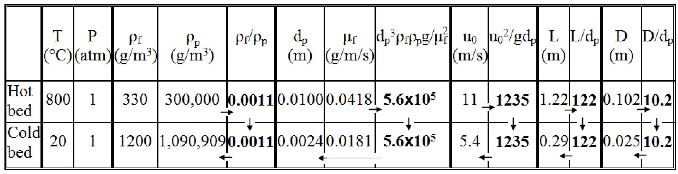
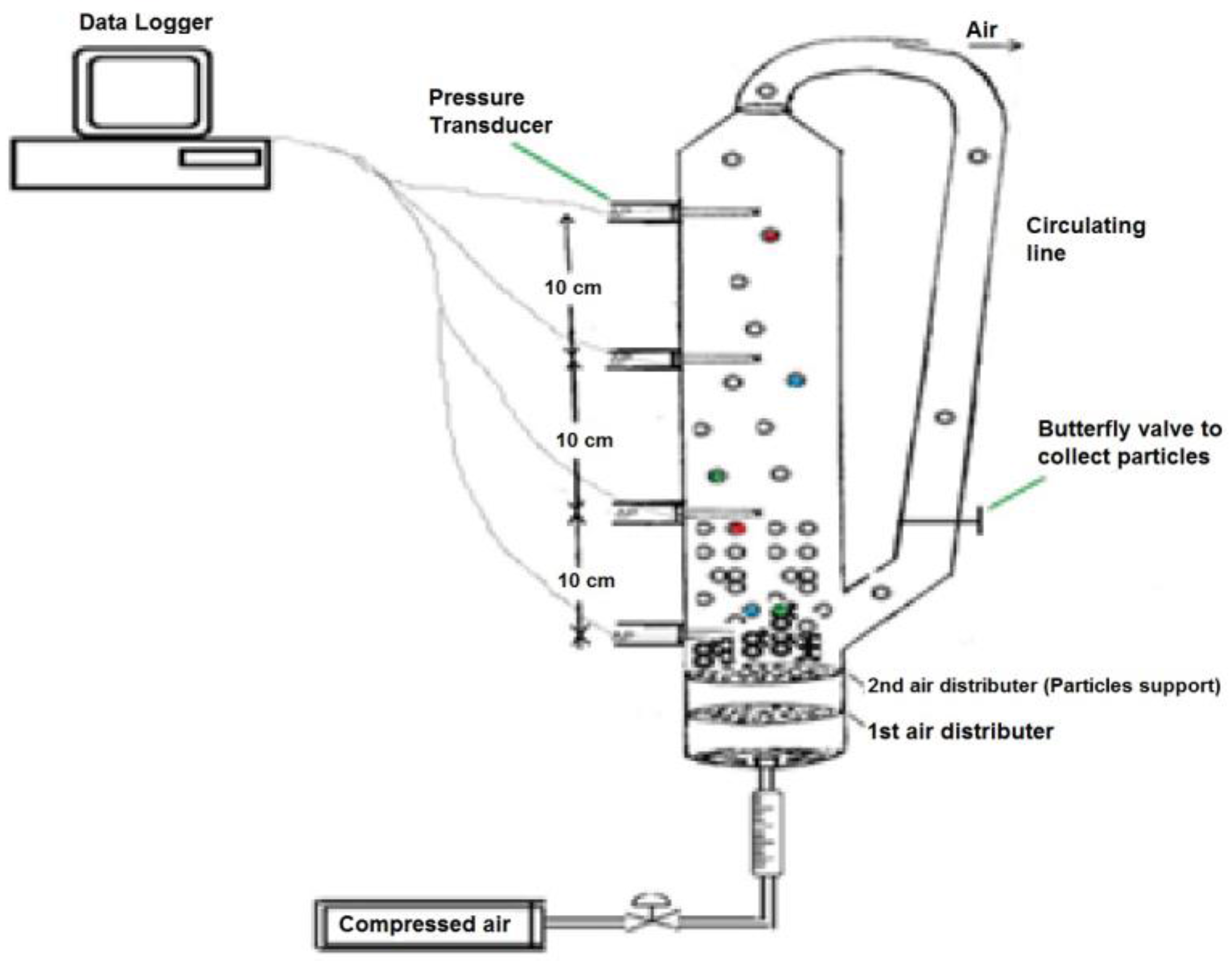
The following is an explanation of the scaling stage to construct the small scale column (See
Figure 1 and follow arrows; note that the sections are divided by thick lines). The type of gas (i.e., its density and viscosity) is known to be ambient air for the cold column; therefore, the density and diameter of particles in this column can be found using the first (
) and second (
) groups in Equation (1b). The third group (
) yields superficial velocity, and the fourth (
) and fifth (
) groups specify
L and
D, height and diameter of the column, respectively.
With some minor relaxations of Geldart’s particle classification [
23],
Figure 1 shows that the scaling rules specify that particles of group B with density >1.1 g/cm
3 (>1.4 g/cm
3 in Geldart’s classification) should be used in the small column to imitate the hydrodynamic behaviour of particles of group A (density < 1.1 g/cm
3) in the large column.
The last three dimensionless groups in Equation (1) were considered as the following: the sphericity (ϕ) of particles in the cold bed was approximately 1; for the fibrous material in the hot bed, it was partially considered as follows: the feeding wheat straw was composed of the particles of approximately 1 to 10 mm length by 1 mm width and 0.2 mm thickness. Accordingly, the sphericity was varied from 0.39 to 0.83.
For particle size scaling, a single value was used (which was scaled from the nominal particle size in the PSD of the large column) rather than having size distribution for spherical particles. Finally, the two bed geometries were identical: both cylindrical, in both columns the probes had similar shapes and installations, and both columns had a ratio of length/diameter ≈ 11.5.
Due to the unavailability of particle size predicted in
Figure 1, particles as close as possible were used (nylon).
Table 1 presents the typical dimensionless numbers for particles of size 2.38 mm and density 1130 kg/m
3. The columns characteristics in
Figure 1 were used for calculations.
Table 1 indicates that the five dimensionless groups (
L/
dp,
D/
dp, ρ
p/ρ
f, ρ
pρ
fdp3g/μ
f2,
u02/
gdp) are nearly equal for the two columns. Such closeness is considered tolerable for this analysis. The Reynolds number (ρ
fu
0dp/μ
f) was also added for an additional confirmation of proper scaling [
13].
If the scaling groups calculated for an atmospheric fluidized bed operating at 800 °C and a model column at ambient condition are equal, the ratio of characteristics of the cold column to the hot column would be: linear dimensions (diameter and height) = 0.25, particle diameters = 0.25, particle densities = 3.5, and superficial air velocities = 0.5 [
24].
Based on the scaling down of the large column data and the above values, a small column of polyethylene with 2.5 cm in diameter and 33 cm in height having a recycling tube was constructed, as shown in
Figure 2. The ambient air was dried, metered, and purged to the bottom of column to fluidize spherical particles. The bulk density of wheat straw (large column) was measured to be very close to 300 kg/m
3. Scaling down criteria resulted in a particle density of 1091 kg/m
3 in the small column. Since particles of exact calculated density were not available, nylon particles with closest density of 1130 kg/m
3 were implemented for further study.
The primary parameters measured in the small column included the minimum fluidization velocity of gas and internal gas pressure. The measurement was carried out in duplicates for verification. Pressure fluctuations were selected as an indicator of fluidizing system dynamics. For the large column two pressure transducers (PX292-005DI, Omega, Stamford, CT, USA) were installed; one 10 cm above the straw feeding port and the other 120 cm above the first one, located below the column outlet. For the small column the pressure transducers (Baratron 220BH-2A1-B-10, MKS Instruments, Andover, MA, USA) were installed at 10 cm intervals along the column with the first one 1 cm above the particle holding screen. Practically, for the small column, the data collected at the top two transducers (shown in
Figure 2) were not utilized because pressures at only heights of 1 and 10 cm were of interest (considering the measurement ports of the large column). The data were recorded by a data logger. Minimum fluidization velocities were estimated by plotting the superficial velocity as a function of pressure drop [
26].
To have a broader experimental verification and insight on the effects of particle density and particle size on the hydrodynamic regime, further experiments were also conducted to include other particle densities and sizes. The densities included 950, 1130, 1350, 1800, and 2200 kg/m3 and the diameters included 2.38, 3.18, 4.76, 6.35, 7.94, and 9.53 mm.
3. Results and Discussion
3.1. Pressure Profiles and Power Spectral Densities
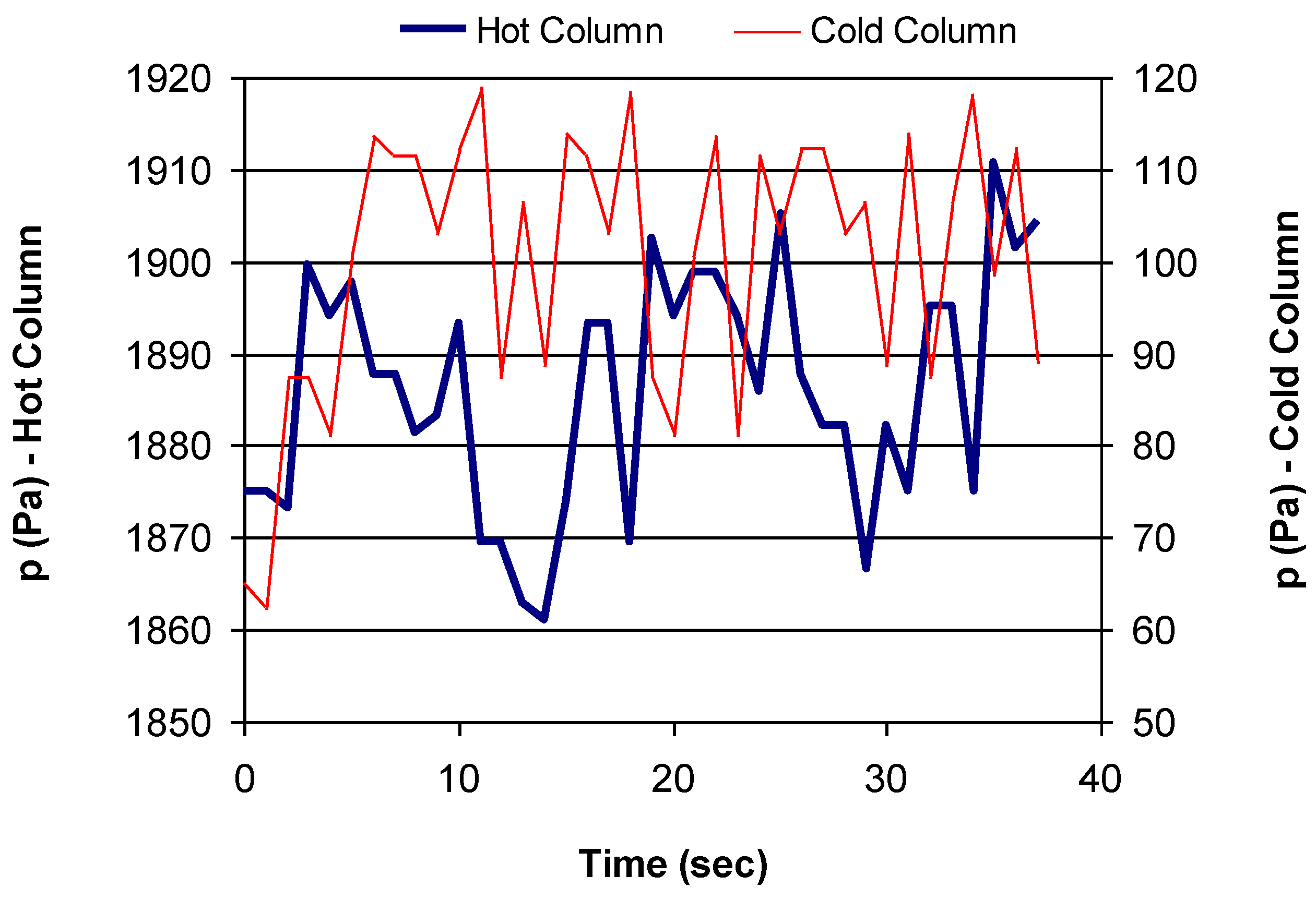
For both large and small columns the pressure differences were measured between the bottom and top transducers. For the hot column the distance between the two instruments was 110 cm and for the cold column the gap was 10 cm. The pressure drops were measured for the entire test, but those corresponding to the fully developed fluidization of particles are shown in
Figure 3. The fluctuations appear to be approximately periodical.
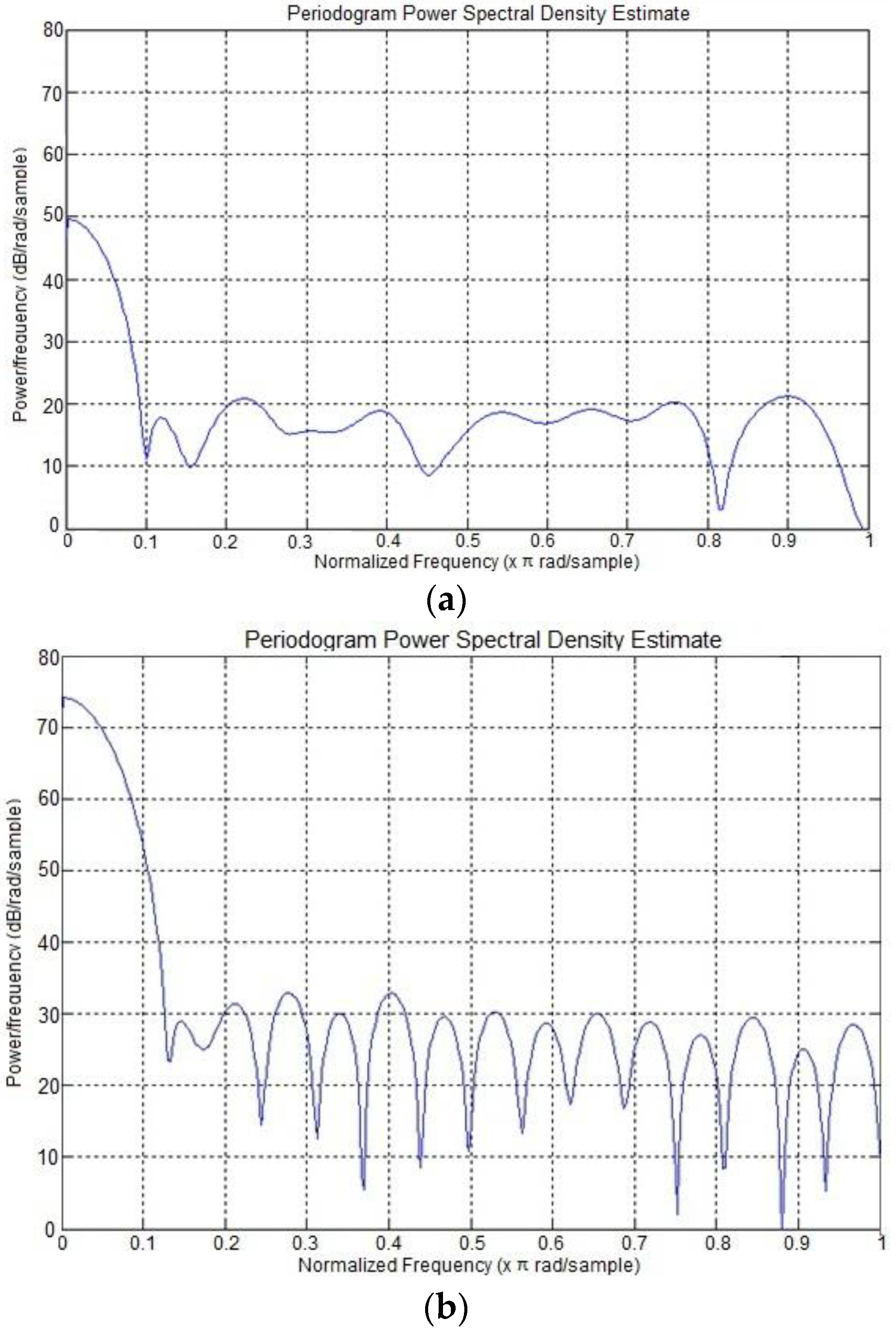
The primary characteristics of pressure signals (frequency and amplitude) were used to generate the power spectral density of pressure fluctuations between the two columns, using Matlab [
22], shown in
Figure 4.
Figure 4 indicates that the frequencies in periodograms (a) and (b) are relatively similar in terms of “peaks and dips occurring at approximately the same time”. As expected, the fluctuations in the hot column are more pronounced and the peaks reach higher values. Comparing the two graphs confirms that due to an approximate similarity between the two periodograms, the pressure fluctuations are similar and hence the hydrodynamic regimes in the hot and cold columns can be deemed somewhat identical.
3.2. Application of Scaling-Law for Velocity Estimation
Generally, two gas velocities in a fluidized bed system are important: gas superficial velocity u0 and gas minimum fluidization velocity umf. The gas superficial velocity was calculated using the input gas flow rate and is important during the entire fluidization stage. In the experiment when particles of 2.38 mm with the density of 1130 kg/m3 reached the height of 10 cm, the air superficial velocity was measured as 5.5 m/s (5.74 ft3/min). The corresponding u0 for a fully developed fluidization in the large column was 11 m/s (cold air inflow of 17 ft3/min before pre-heating).
umf in the small column was estimated by plotting pressure drop across the bed versus superficial velocity. For this purpose one end of the lower transducer was left open to the atmosphere, so the transducer measured the change in the gauge pressure just above the bed when air flow rate varied. For instance, for the selected particles (nylon of size 2.38 mm and density 1130 kg/m3) air flow rate and pressure were recorded. Commencing from zero and increasing air flow rate, pressure drop increases to a maximum which is just before bed expansion. By further increase in the air flow rate the pressure drop continues to decrease until reaching a minimum after which pressure drop increases again.
For nylon particles of 2.38 mm and 1130 kg/m
3 when volumetric flow rate increased to 1.09 ft
3/min (
u0 = 1.05 m/s) the particles reached incipient of fluidization; hence for those particles
umf = 1.05 m/s. Monitoring (at duplicates) of the pressure profiles for all particles (different sizes and densities) provided their
umf.
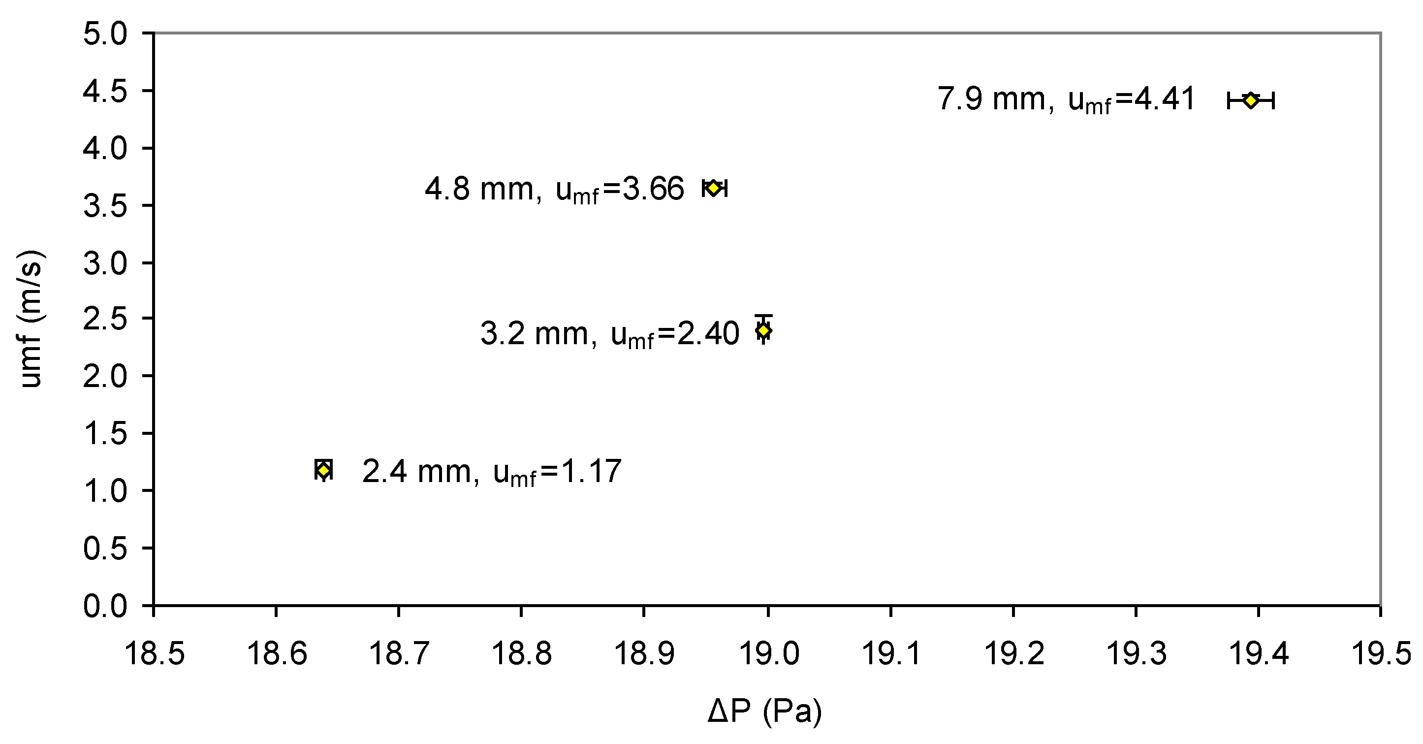
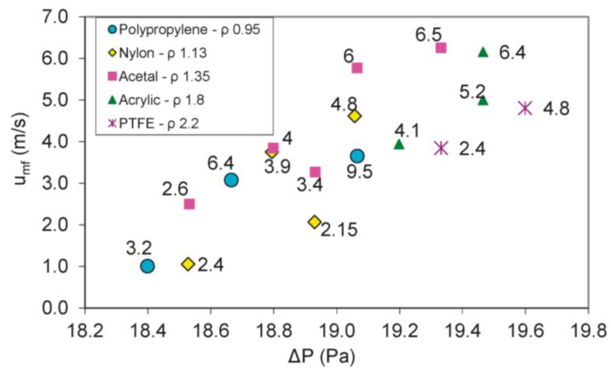
Figure 5 presents the results of
umf versus the pressure drop right at the
u0 =
umf.
Figure 5 indicates that for one type of particles (density fixed) but different sizes,
umf has increased with increasing pressure drop. The data in
Figure 5 are moderately scattered, although they show a reasonable trend. Generally, the relationship between pressure drop, minimum fluidization velocity, density, and particle size is highly non-linear. Shortly in the text, the Ergun equation [
24] is used to predict
umf for comparison with the measurements.
As mentioned,
umf and ΔP were measured twice at each case to evaluate reproducibility of the data collection method.
Figure 5 also presents the variation in the measurement of the two variables for some selected particles. Based on
Figure 5 data, using the method of graphing
u0 vs. ΔP to estimate
umf involves 3%–14% variation in velocity and 1%–2% variation in pressure drop measurements (
Figure 6). The negligible variability in pressure but higher variability in
umf were expected as the former was instrumentally measured and the latter was visually estimated.
The following approach provides theoretical estimation of
umf using the Ergun equation [
26,
27]. This equation, when
ugas is replaced by
umf and ε (voidage) is replaced by the voidage at fluidizing incipient (ε
mf), yields:
A proper relationship between particles sphericity (φ) and ε
mf such as Equation (3) can be utilized:
According to CoulsonandHarker [
26] and after some manipulation of Equation (18) together with Equation (19) the following equation is found for a wide range of φ
s and ε
mf.
Using the definition of Reynolds number,
umf can then be found:
Adopting this approach, Remf for nylon particles ( = 1.13 g/cm3, dp = 2.38 mm) was found to be 183, resulting in umf to be 1.16 m/s, a value quite close to the measured minimum fluidizing velocity of 1.05 m/s. Note that the measured value is based on a simple visual inspection and is subject to potential errors, although velocity measurements were carried out in duplicates and the results are the average of the two measurements.
It is notable also that Ergun equation can be directly used to calculate
umf. However, the purpose in using this indirect method is to make use of Ar and Re numbers, the non-dimensional groups used in scaling up which are hydrodynamic indicators of the system (
Table 1).
The results presented above indicated that for the small column when nylon particles (as scaled particles) were utilized, the umf was relatively accurately predicted by Equations (4) and (5). Therefore the approach can be used for the large column calculations as well.
3.3. Application of Froude Numbers
Stein et al. [
16] showed that if between two columns Froude numbers (Fr =
or
or the square of them) are equal, then their particle circulation frequencies are equal too. The Fr was calculated between the two columns and was presented in
Table 2.
Comparing the last two columns of
Table 2 reveals that for the two fluidized systems the calculated values of Fr are approximately equal, hence roughly the similarity of particle circulation frequencies in the two columns.
Particle size distribution has been recommended as one of the scaling parameters to be matched between the two systems [
13]. In this work, particle size distributions between the two models were not completely adjusted which is a source of error. Coulson and Harker [
27] stated that “in the absence of channeling, it is the shape and size of the particles that determine both the maximum porosity and the pressure drop across a given height of fluidized bed of a given depth”. It was implied that since there was not any channeling during the experiments we could approximately assume that pressure drop and pressure fluctuation due to particles of one size (the average size) is equal to the pressure drop/fluctuation due to the particles of varying size. Although it is a limitation in this study, the effects of this assumption will not be significant compared to the effects of other crucial parameters such as particle velocities and densities.
3.4. CFD Simulation Results
2D CFD models were established in ANSYS Fluent 14.0 to simulate the hydrodynamics of the “cold” column. Three cases with , and as Case 1, , and as Case 2, and , , and as Case 3 were established.
The CFD models were solved by the finite volume method in ANSYS Fluent 14. A grid with 9500 cells was applied to the CFD model. The Green-Gauss cell based method was used to calculate the gradient of the variables. The scheme of phase coupled SIMPLE was applied to couple the velocity and pressure. The convergence criterion was 0.001 and the time step was set as 1.0 × 10
−4. The simulation time is set as 40 s. The simulation results are averaged between 20 and 40 s to obtain stable values in the steady-state. The computation was conducted on a cluster of the High Performance Computing Virtual Laboratory (HPCVL) using 12 Intel X5670 cores at 2.9 GHz. The model settings are shown in
Table 3. For the details of the governing equations in the CFD models, please refer to
Appendix A.
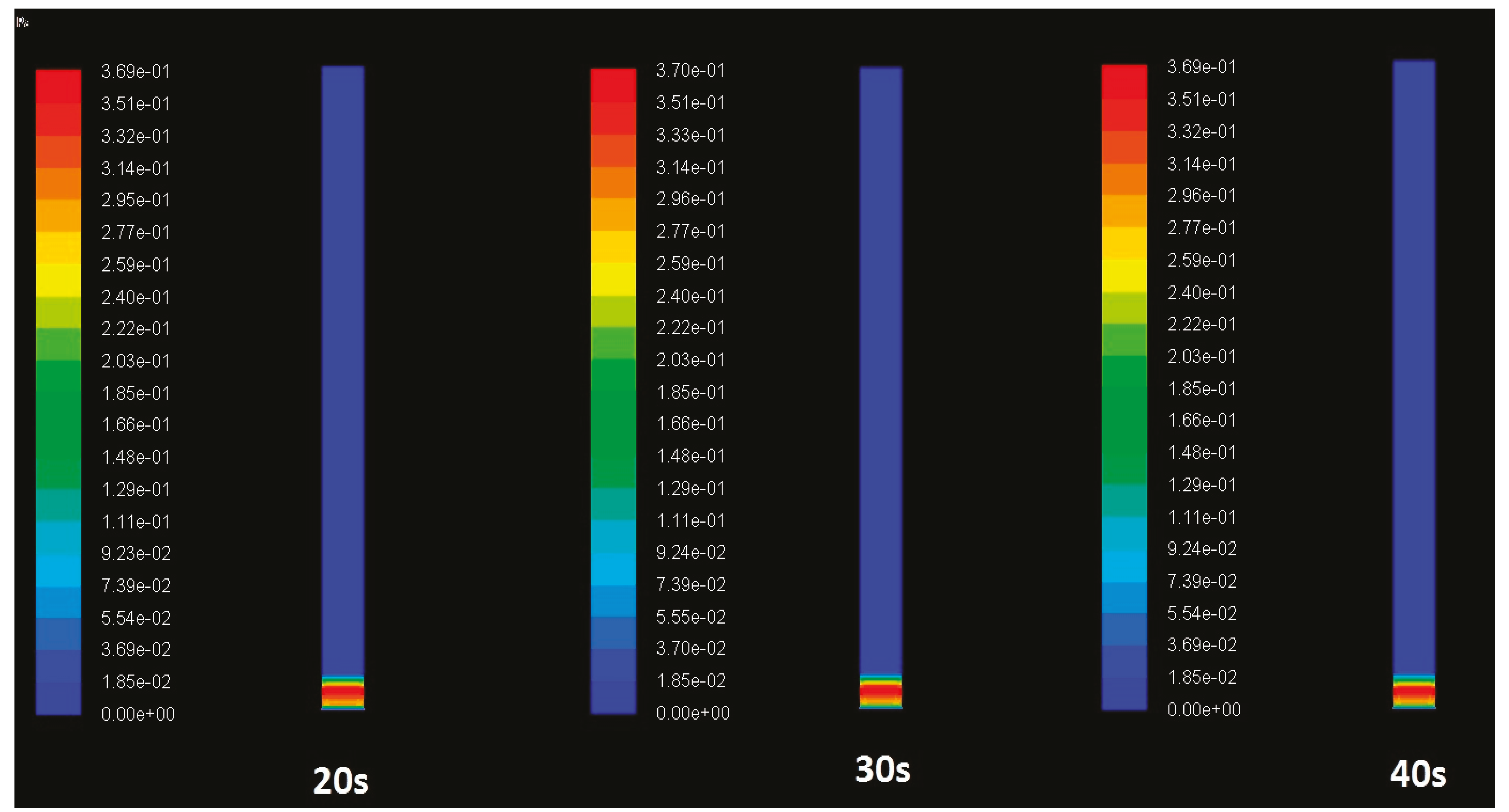
The solids volume fraction contours of case 1 are shown in
Figure 7. Since the gas velocity of 1.92 m/s is close to the minimum fluidization velocity, only minimum fluidization was predicted in the model, which matches our observation in the experiment.
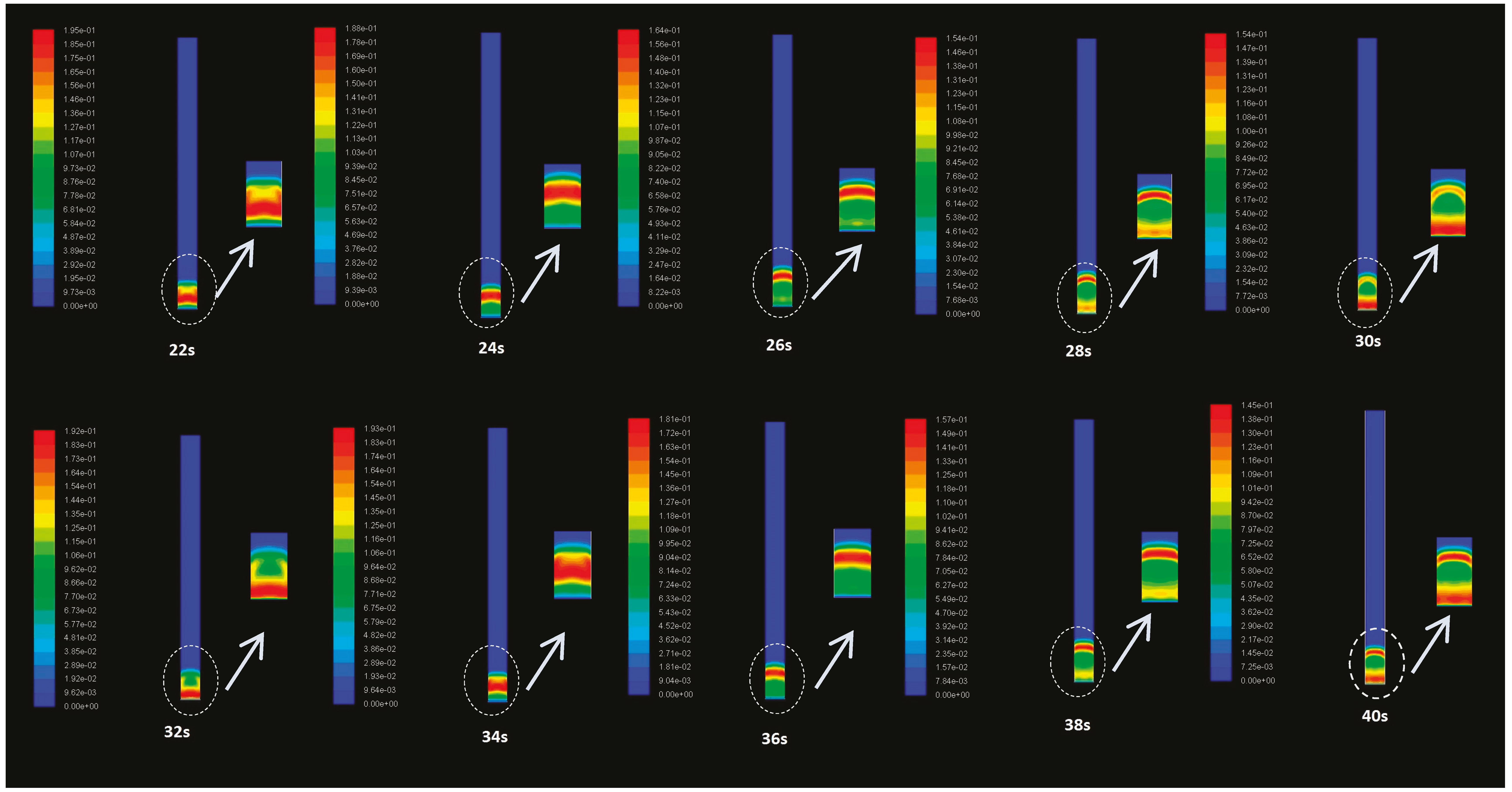
Figure 8 demonstrates the solids distribution between 20 and 40 s for Case 2. It can be seen that when the gas velocity increases to 5.5 m/s, solids are fluidized by air at the bottom of the column and the solids bed expands. Gas bubbles are formed and rise through the solids bed.
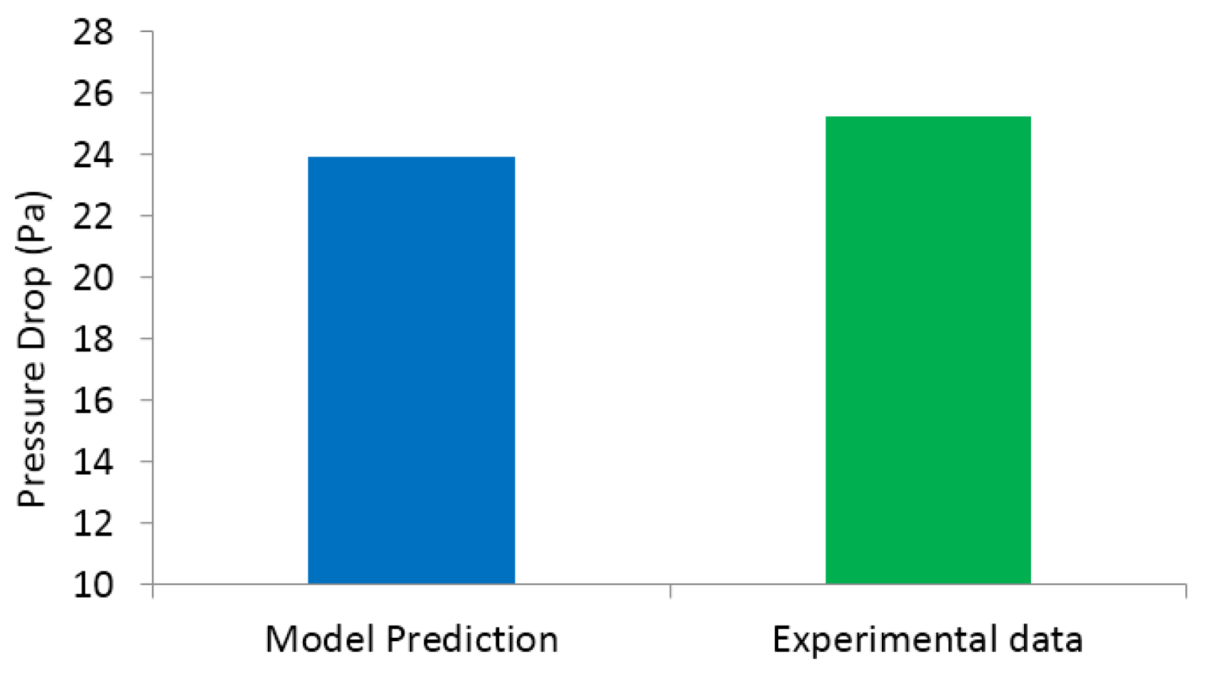
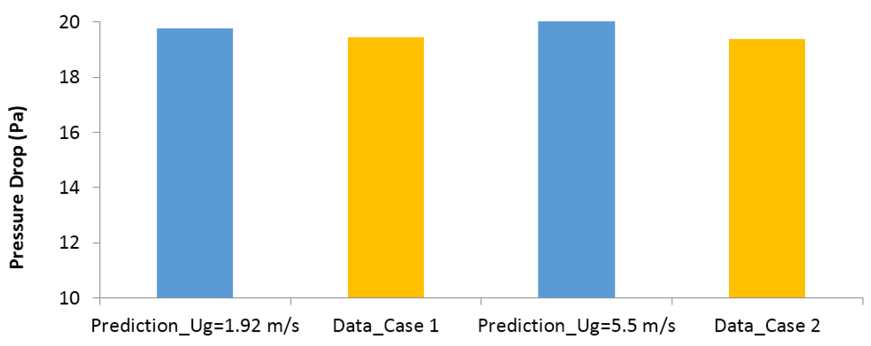
In
Figure 9, the predicted pressure drops of Cases 1 and 2 are compared with the measured values in the experiment. As shown in the figure, the simulation results of Case 1 and 2 are both consistent with the experimental data. Additionally, the pressure drop from case 1 with the minimum fluidization is close to the pressure drop from case 2 with fully developed fluidization, which matches the observations by other researchers [
28,
29,
30] that in fluidized-bed reactors after the minimum fluidization was reached, the bed kept expanding with the increase of gas velocity, while the pressure drop remained constant.
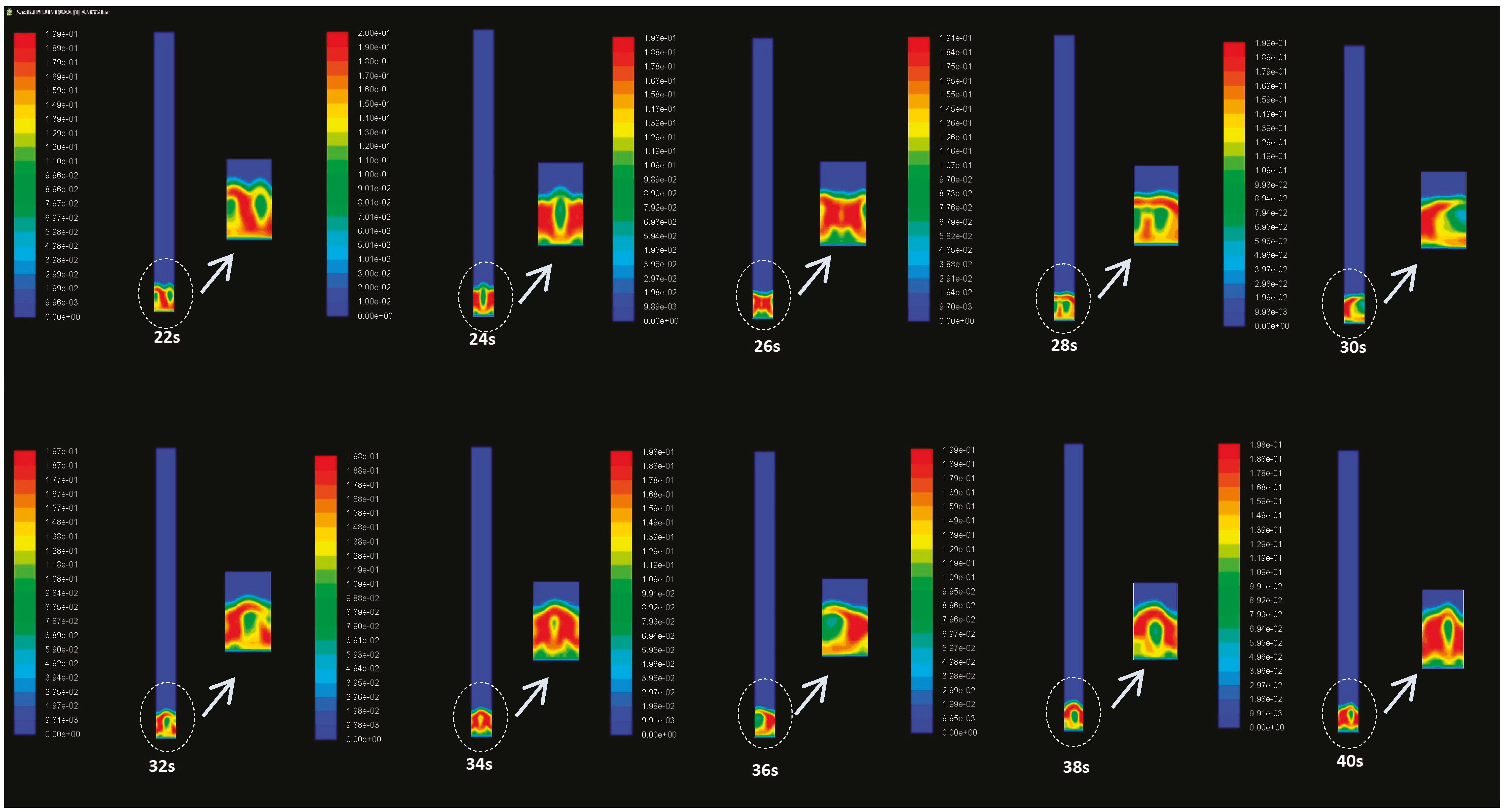
The solids distribution in the column for Case 3 between 20 and 40 s is shown in
Figure 10. As seen in the figure, bubbles are generated after air is injected to the bottom of the column. The structure of solids slugging was also predicted in Case 3: the solids concentration is high in the central core region while the solids concentration becomes dilute in the near-wall region. The solids slugging may be due to bubble coalescence, high gas velocity and relatively small particles. The solids slugging can cause significant fluctuation in solid fluidization and is not recommended for normal operation of fluidized-bed reactors; however, as indicated by Kashyap et al. [
30], solids slugging can provide some advantages such as avoiding solids back-mixing in the near-wall region and gas bypassing the central core region. The solids slugging structure can be measured with the technology of gamma ray densitometry [
30,
31]. Other techniques such as particle image velocimetry (PIV), laser doppler anemometry (LDA), and fiber optic probe can also be used for the measurement of solids structure in fluidized-bed reactors [
31,
32,
33,
34]. In this work the measurement of solids concentration was not done due to lack of these advanced measuring instruments; however, the measurement of solids concentration will be included in our future studies to improve the quality of our research.
It is also seen that the solids bed in Case 3 expands further than that of Case 2. It is known that gas velocity, particle diameter, and solid density play important roles in solid fluidization. Given the fact that the gas velocities are the same and the solid densities are similar in Cases 2 and 3, the different fluidization patterns are mainly caused by the different diameters. Smaller particles of 2.38 mm in Case 3 tend to be carried up more easily by the gas than large particles of 3.18 mm in Case 2.
Figure 11 shows the comparison of simulation results and experimental data and the model prediction of Case 3 demonstrates good agreement with experimental data, indicating that the current CFD model is capable of predicting the accurate flow pattern in the “cold” gasifier.


