Combined Two-Stage Stochastic Programming and Receding Horizon Control Strategy for Microgrid Energy Management Considering Uncertainty

Abstract

Microgrids (MGs) are presented as a cornerstone of smart grids. With the potential to integrate intermittent renewable energy sources (RES) in a flexible and environmental way, the MG concept has gained even more attention. Due to the randomness of RES, load, and electricity price in MG, the forecast errors of MGs will affect the performance of the power scheduling and the operating cost of an MG. In this paper, a combined stochastic programming and receding horizon control (SPRHC) strategy is proposed for microgrid energy management under uncertainty, which combines the advantages of two-stage stochastic programming (SP) and receding horizon control (RHC) strategy. With an SP strategy, a scheduling plan can be derived that minimizes the risk of uncertainty by involving the uncertainty of MG in the optimization model. With an RHC strategy, the uncertainty within the MG can be further compensated through a feedback mechanism with the lately updated forecast information. In our approach, a proper strategy is also proposed to maintain the SP model as a mixed integer linear constrained quadratic programming (MILCQP) problem, which is solvable without resorting to any heuristics algorithms. The results of numerical experiments explicitly demonstrate the superiority of the proposed strategy for both island and grid-connected operating modes of an MG.

1. Introduction

Microgrids (MGs) are micro power systems integrating a number of loads and distributed energy resources (such as photovoltaic (PV), wind, storage systems, controllable distributed generators (DGs), and controllable loads) [1]. An MG can operate in both grid-connected or island-mode by connecting and disconnecting from the grid. The potential to integrate intermittent renewable energy sources (RES) in a flexible and decentralized way makes the concept of MGs more attractive. Because of the randomness in power production of RES, load demand, and the electricity price, in addition with the state transitions over the entire time frame of MG energy management caused by the buffering effect of energy storage devices, the optimal operation of MGs comes to be highly computationally complex and challenging.

Although, many kinds of forecast methods have been proposed for forecasting the load demand, wind, PV generation and electricity price, a point forecast is always subject to error and the probability that the forecasting scenario occurs is clearly close to zero. Thus, a deterministic approach will affect the performance of the power scheduling and the operating cost of an MG. The studies considering uncertainty for MG energy management can be categorized into two groups [2]: robust optimization based approaches [2,3,4] and stochastic optimization based approaches [5,6,7,8]. In [3], an MG energy management framework for the optimization of individual objectives of MG stakeholders is proposed. The optimal scheduling strategy is achieved by using a robust optimization approach which considers the uncertainties related to the power output of renewable generators and quantify the uncertainties by prediction intervals. Recently, two-stage stochastic programming (SP) has also been applied to MG energy management [5,6,7,8] and it is demonstrated to be a flexible and effective strategy to deal with the uncertainty in MG. For two-stage SP, stochastic variable scenarios are always generated through Monte Carlo simulation (MCS) [5]. By considering all possible realizations of each scenario, the risk cost dues to imprecise forecast of stochastic variable is reduced. In [7], a two-stage SP strategy is applied for the energy and reserve scheduling with demand response. In [5], a two-stage SP method for the optimal design of distributed energy system is proposed. Niknam et al. [8] proposes a stochastic model for optimal energy management with the goal of cost and emission minimization and the proposed model is solved by using a complex heuristics algorithm. However, the forecast errors increased as the forecasting time horizons become longer [9,10,11,12], and the SP based open loop strategy cannot deal with the forecast errors effectively without using the updated forecast information. Thus, only with SP strategy, the forecast uncertainty in MG cannot be effectively depressed.

Recording horizon control (RHC), also known as model predictive control (MPC), as an advanced method for process control, has also been used in the power system as it can incorporate both forecasted and newly updated information to make decisions [13,14]. In [15], with timely updated wind and market price forecasts, RHC is used for the dispatch of hydrogen storage together with a wind power plant. In [16,17,18], an RHC scheme is proposed to minimize the operating cost of an MG. In [19], an RHC-based power dispatch approach is proposed to minimize the operational cost while accommodating the plug-in electric vehicles (PEV) charging uncertainty by timely update the predictive model. However, all of these methods are deterministic approaches, which do not consider all the possible forecast errors related to load demand, PV and wind power production, and electricity price in the optimization model, which naturally affects the result accuracy and therefore the overall performances of MG.

In this paper, a combined two-stage SP and RHC strategy, named SPRHC, is proposed for microgrid energy management under uncertainty. For the SPRHC strategy, it combines the advantage of SP and RHC by considering the forecast errors through SP and involving a feedback mechanism through RHC with the recently updated forecast information. Thus, the proposed SPRHC strategy can effectively avoid short sighting and further compensate the uncertainty in MG. Through the two-stage SP, the power scheduling decisions are divided in two stages. The first-stage decisions (such as the unit commitment of DGs and the charging/discharging schedule of battery storage system) are made prior to the observation of the random scenarios, while the second-stage decisions (such as the economic power dispatch of committed DGs, power exchange between MG and the utility, the load shedding, and the power generation curtailment) are made adaptively according to the first-stage decisions and the observation of the real scenario. The optimization model involves the forecast uncertainty of load demand, PV and wind production, and electricity price. The complicated SP problem is transferred into a deterministic optimization problem with multiple deterministic scenarios generated by MCS strategy. In order to reduce the computational burden, a scenario reduction method named backward reduction algorithm (BRA) [20] is applied to remove the similar scenarios and keep a good approximation of the uncertainty. In order to further compensate the uncertainty within the MG energy management, a feedback mechanism based on RHC is proposed to be incorporated with two-stage SP. The results of numerical experiments explicitly show benefits of the proposed strategy for an MG operating in both grid-connected and island operating modes.

The main contributions of this paper are: (1) the forecast errors of load demand, PV and wind power production, and electricity price are considered for MG energy management and the problem is formalized into a two-stage SP; (2) An RHC based feedback mechanism is combined with SP strategy by using the lately updated forecast information, which can effectively avoid short sighting and further compensate the uncertainty; (3) In order to avoid the simultaneous charging and discharging of battery systems, a proper strategy is proposed to guarantee a correct behavior while keeping the model as a mixed integer linear constrained quadratic programming (MILCQP) model, which is solvable without resorting to any heuristics algorithms; (4) The superiority of the proposed SPRHC strategy is demonstrated through case studies that involve both island mode cases and grid-connected mode cases.

This paper’s order is as follows. In Section 2, scenario generation and reduction strategy is proposed. Section 3 proposes the two-stage SP formulation for MG energy management. In Section 4, RHC is introduced. Section 5 shows the numerical experiments. Finally, the conclusions are given in Section 6.

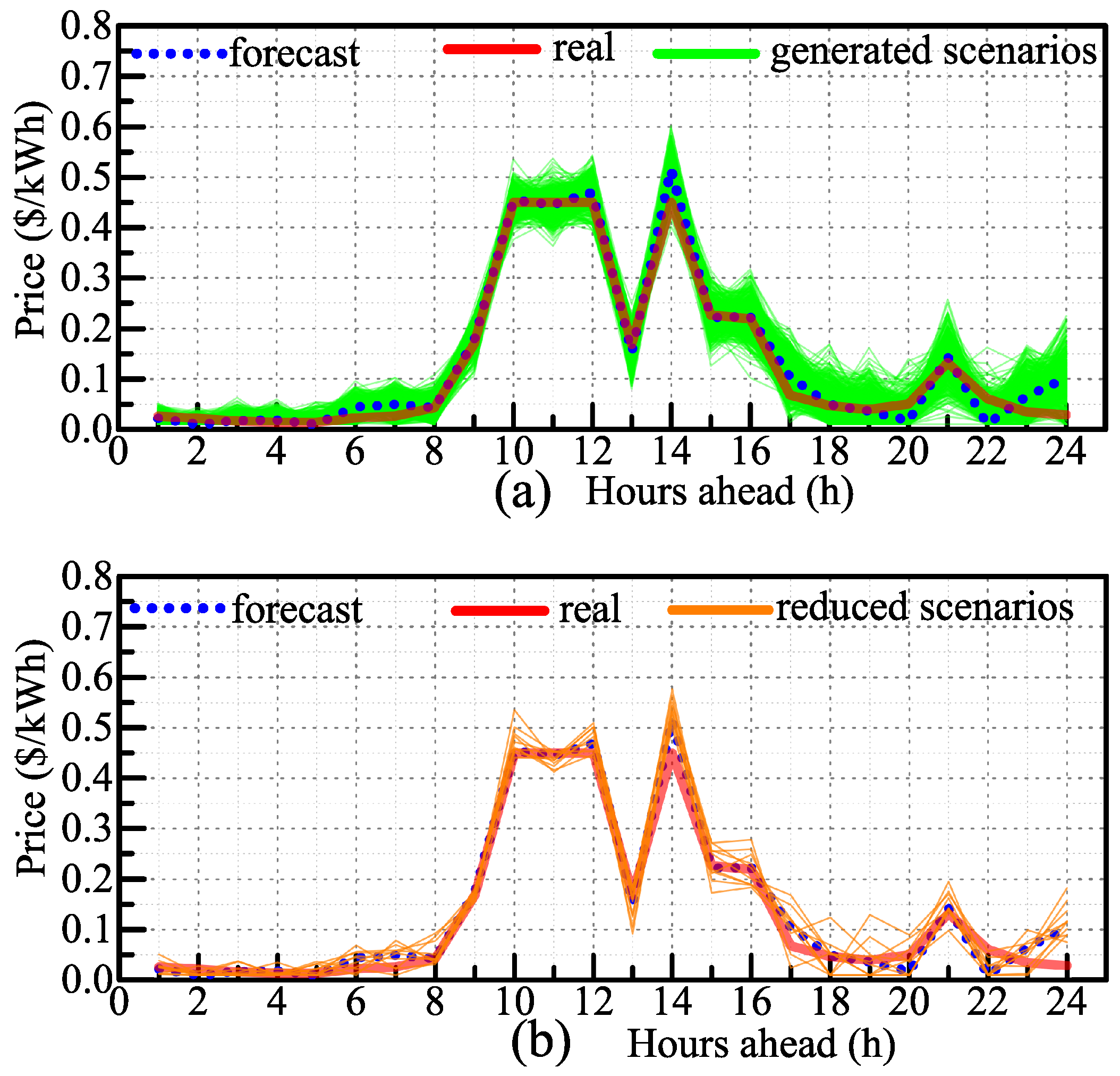
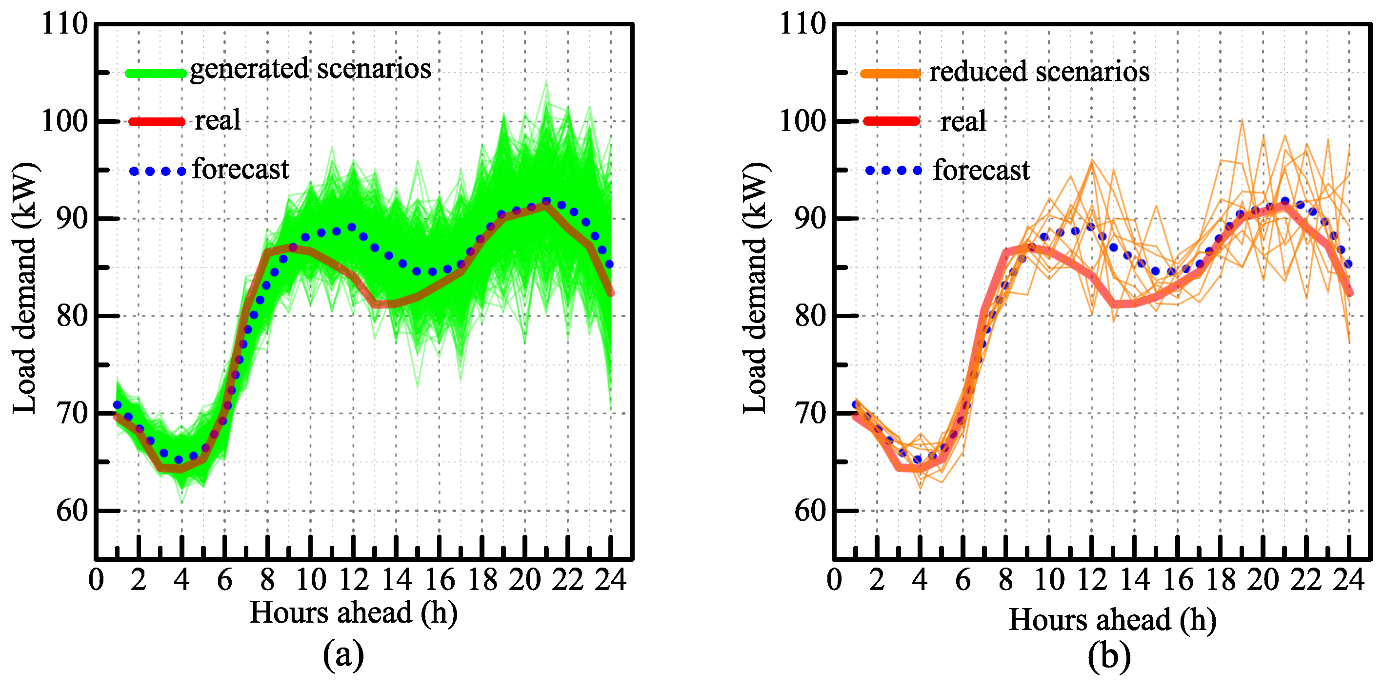
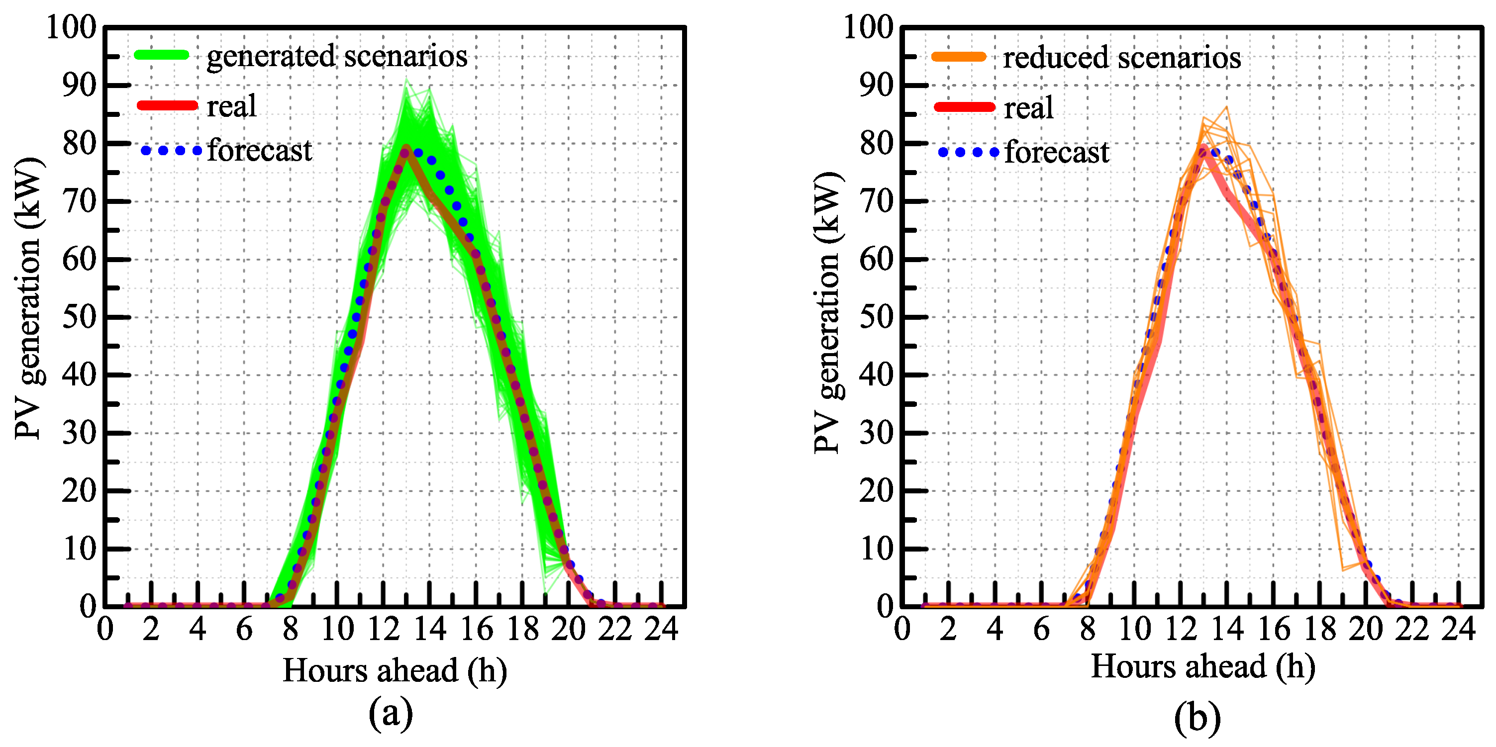
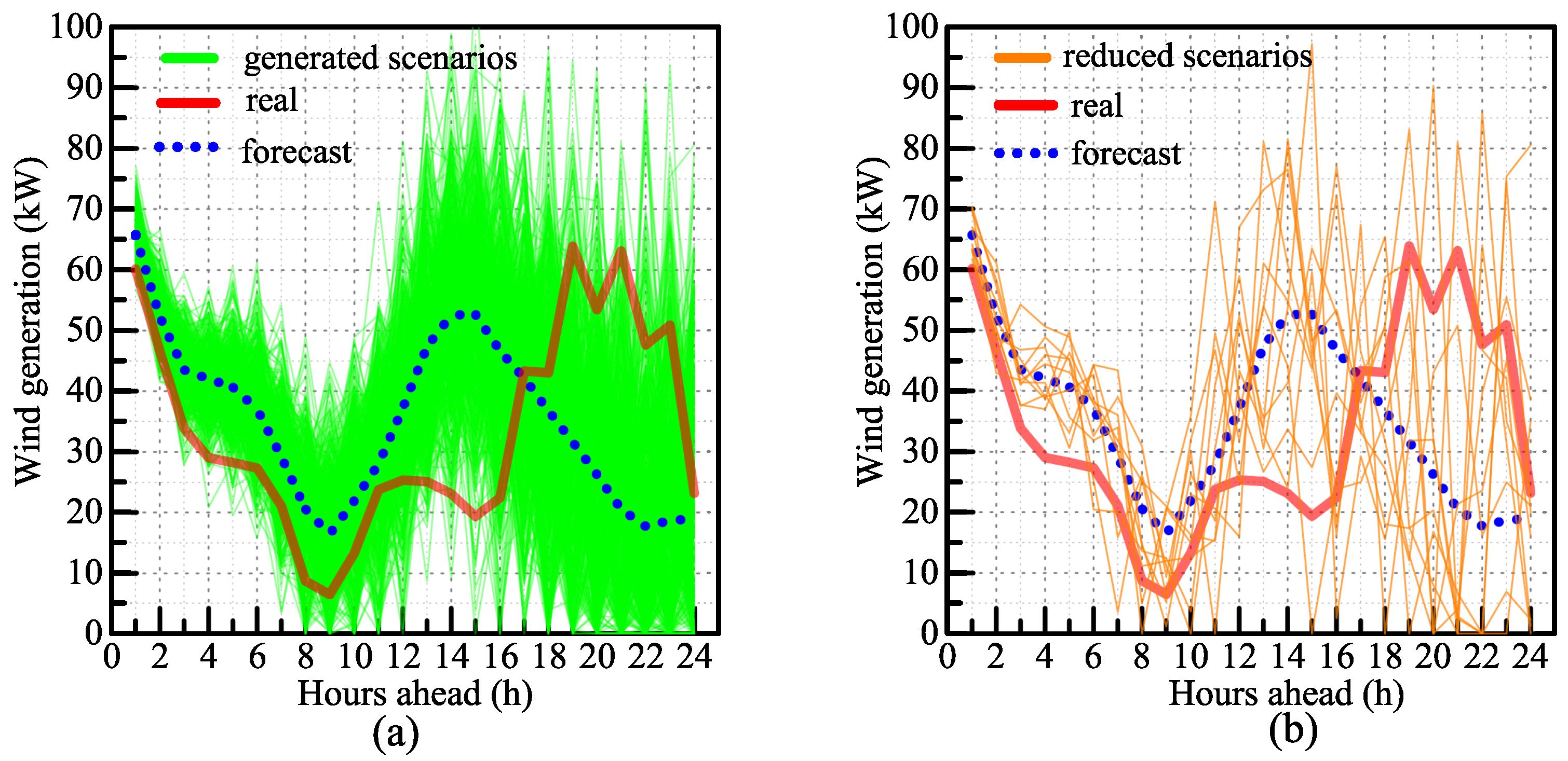
2. Scenario Generation and Reduction

2.1. Modeling the Uncertainty in an MG

Many kinds of forecast methods have been proposed for forecasting the load demand, wind and PV generation, and electricity price related with different time horizon periods (1 h ahead, 2 h ahead, and so on) [9,21,22,23,24,25,26]. However, the probability that the forecasting scenario occurs is clearly close to zero, since a point forecast is always subject to an error [27]. Therefore, SP is applied to reduce the risk costs due to imprecise forecast by considering several possible realizations of each scenario. For SP, the scenarios of random variables (such as load demand, wind and PV generation, and electricity price) should be firstly generated according to its probabilistic characteristics. However, it is hard to directly find out their probabilistic characteristics since they involve many random factors, such as illumination intensity, cloud cover, temperature variations, etc. [6]. Generally, the forecast error of load demand, wind and PV generation, and electricity price are fitted well to certain standard probabilistic distribution [28]. Thus, the forecast error models are applied for scenario generation.

In most literature, the normalized forecast error of load demand, wind and PV power production, and electricity price are assumed to follow the normal distribution [29,30], i.e., $e\sim N(0,\mathsf{\delta })$. Furthermore, as shown in [9,10,11,12,25,26], for the forecasts of load demand, wind and PV generation, and electricity price, longer time horizon periods present larger forecast errors (here described by larger normalized standard deviation values) and the forecast errors depend significantly on the forecast methods [9]. In this paper, the MCS [31] approach is used to generate stochastic variable scenarios for a certain time horizon according to time-horizon-dependent empirical probability distribution functions (PDFs) of forecast error, as shown by (1) to (4).

$$e_{t,s}^{PV}\sim N(0,{\mathsf{\delta }{}_t^{PV}}^2),P_{t,s}^{PV}=P_t^{PV\_f}\times (1+e_{t,s}^{PV}),$$

(1)

$$e_{t,s}^{Wind}\sim N(0,{\mathsf{\delta }{}_t^{Wind}}^2),P_{t,s}^{Wind}=P_t^{Wind\_f}\times (1+e_{t,s}^{Wind}),$$

(2)

$$e_{t,s}^{Load}\sim N(0,{\mathsf{\delta }{}_t^{Load}}^2),P_{t,s}^{Load}=P_t^{Load\_f}\times (1+e_{t,s}^{Load}),$$

(3)

$$e_{t,s}^{Price}\sim N(0,{\mathsf{\delta }{}_t^{Price}}^2),Pric{e}_{t,s}^{import}=Pric{e}_t^{import\_f}\times (1+e_{t,s}^{Price}).$$

(4)

It should be noted that the forecast errors depend significantly on the forecasting techniques [9] and the forecasting techniques play an important role in the operation of proposed approach; however, the development of such forecasting techniques is outside the scope of this paper. Thus, the analysis of the performance of the forecasting techniques is not discussed here. Without loss of generality, the standard deviations (${\mathsf{\delta }}_t^{PV}$, ${\mathsf{\delta }}_t^{Wind}$, ${\mathsf{\delta }}_t^{Load}$, and ${\mathsf{\delta }}_t^{Price}$) are assumed to be linearly increasing with the distance from current time step, as shown by (5) to (8):

$${\mathsf{\delta }}_t^{PV}=\left(T\times {\mathsf{\delta }}_1^{PV}-{\mathsf{\delta }}_T^{PV}+t\times ({\mathsf{\delta }}_T^{PV}-{\mathsf{\delta }}_1^{PV})\right)/\left(T-1\right),$$

(5)

$${\mathsf{\delta }}_t^{Wind}=\left(T\times {\mathsf{\delta }}_1^{Wind}-{\mathsf{\delta }}_T^{Wind}+t\times ({\mathsf{\delta }}_T^{Wind}-{\mathsf{\delta }}_1^{Wind})\right)/\left(T-1\right),$$

(6)

$${\mathsf{\delta }}_t^{Load}=\left(T\times {\mathsf{\delta }}_1^{Load}-{\mathsf{\delta }}_T^{Load}+t\times ({\mathsf{\delta }}_T^{Load}-{\mathsf{\delta }}_1^{Load})\right)/\left(T-1\right),$$

(7)

$${\mathsf{\delta }}_t^{Price}=\left(T\times {\mathsf{\delta }}_1^{Price}-{\mathsf{\delta }}_T^{Price}+t\times ({\mathsf{\delta }}_T^{Price}-{\mathsf{\delta }}_1^{Price})\right)/\left(T-1\right).$$

(8)

Thus, the forecast errors of $e_{t,s}^{PV},e_{t,s}^{Wind},e_{t,s}^{Load}$, and $e_{t,s}^{Price}$ are generated by a random number generator of normal distribution with standard deviation linearly increasing with the distance from current time step, which is in accordance with the forecast error distribution model.

According to the generated forecast errors through MCS, a certain number (such as $N_0$) of scenarios are generated, and each scenario consists of a vector as shown by (9) and with the probability $\raisebox{1ex}{$1$}\!\left/ \!\raisebox{-1ex}{$N_0$}\right.:$

$$X_s=\left[P_{1,s}^{PV},...,P_{T,s}^{PV},P_{1,s}^{Wind},...,P_{T,s}^{Wind},P_{1,s}^{Load},...,P_{T,s}^{Load},P_{1,s}^{Price},...,P_{T,s}^{Price}\right].$$

(9)

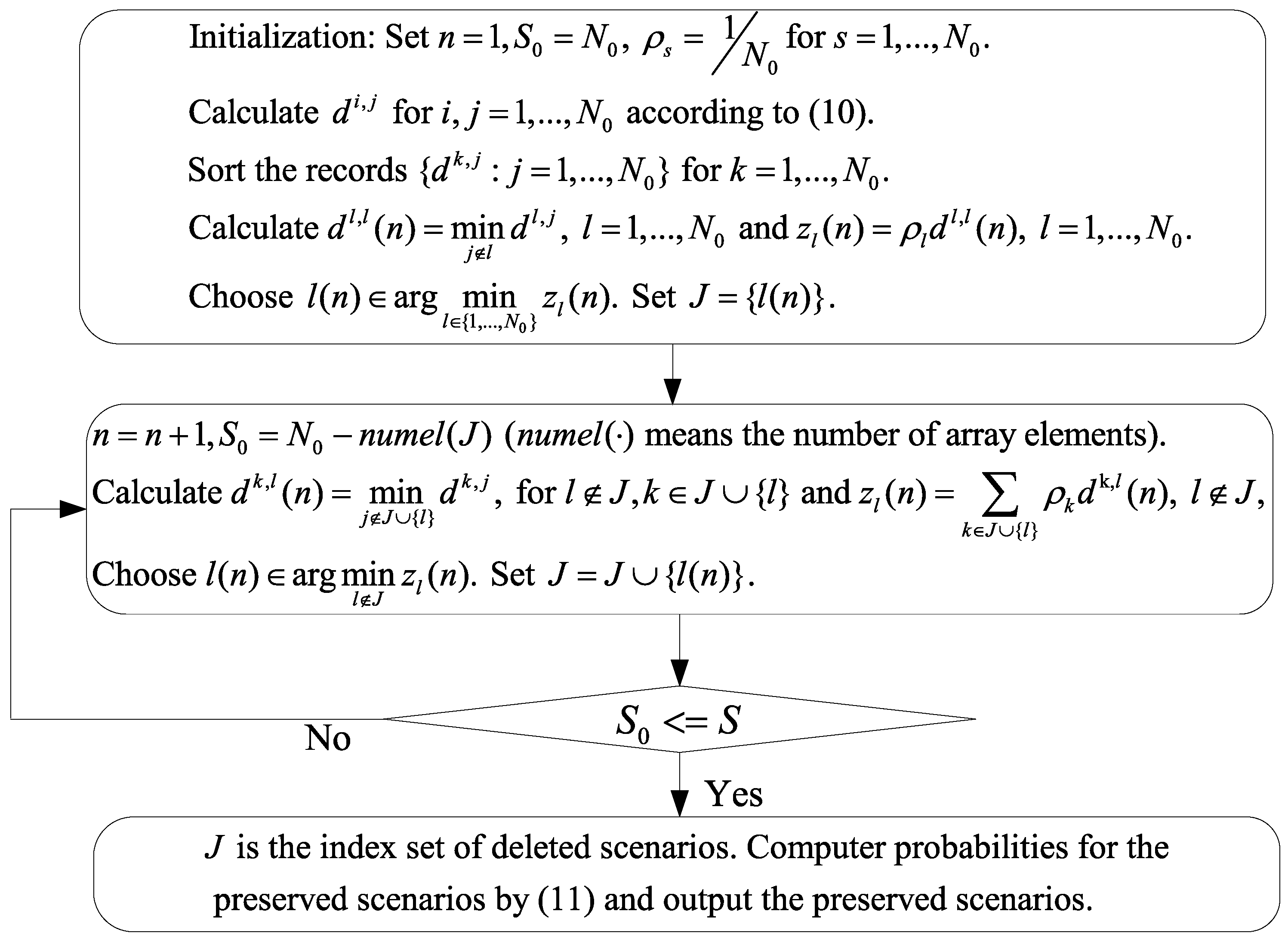
2.2. Scenario Reduction

In addition, a higher number of scenarios can result in a better modeling of the uncertainty in an MG, but it is at the expense of increasing the computational burden. Thus, a scenario reduction method is needed to remove the similar scenarios and keep a good approximation of the uncertainty. The backward reduction algorithm (BRA), which has been proven to provide very good performances in the two-stage mixed integer stochastic programming [13], is adopted in this paper. The diagram of BRA [20] is shown in Figure 1.

Let the distance between two scenarios be described as a two-norm, as shown in (10):

$$d^{i,j}=∥X_i-X_j∥.$$

(10)

Then, the BRA is implemented until S scenarios are remaining. The probabilities for the preserved scenarios can be calculated by (11):

$${\mathsf{\rho }}_j={\mathsf{\rho }}_j+\sum _{i\in J_j}{\mathsf{\rho }}_i,\text{for}\text{each}j\notin J,where{J}_j=\{i\in J:j=j\left(i\right)\}andj\left(i\right)\in arg\underset{j\notin J}{min}{d}^{i,j}foreachi\in J.$$

(11)

3. Two-Stage Stochastic Programming Formulation for Microgrid Energy Management

The multi-stage SP model [32,33,34] allows revision of the planning decisions sequentially when the uncertainty realized hourly [33]. However, for the multi-stage SP model, the problem becomes extremely large when the number of stages increase [32], even though a relatively small number of nodes are allowed in each stage. With an RHC strategy, as proposed in the next section, the two-stage SP model can also sequentially make the decisions with hourly updated forecast information, which compensates for the lack of additional stages for uncertainty unveiling. Thus, the two-stage SP model is applied in this paper. In order to consider the forecast error of the load demand, PV and wind power production, and electricity price for the MG energy management under uncertainty, a two-stage stochastic programming formulation is developed in this section.

3.1. Objective Function

The operation cost of an MG consists of the start-up/shut-down cost and fuel cost of controllable DGs, degradation cost of battery, load shedding cost, and power generation curtailment cost. In a grid-connected mode, the operation cost of an MG also contains the cost of power purchased from the utility minus the profit gained by exporting power to the utility. Considering the uncertainty of load demand, PV and wind power generation, and electricity price, the costs of MG can be formulated as a two-stage objective function as shown in (12):

$$\begin{array}{c}\text{Min}f={\displaystyle \sum _{t=1}^T}\left\{{\displaystyle \sum _{i=1}^{N^{DG}}}\left(u_{i,t}^{SU}\times S{U}_i^{DG}+u_{i,t}^{SD}\times S{D}_i^{DG}+(P_t^{Char}+P_t^{DisChar})\times \Delta t\times Pric{e}^{Bat}\right)\right\}\hfill \\ +{\displaystyle \sum _{s=1}^S}\left\{{\mathsf{\rho }}_s\times \Delta t\times {\displaystyle \sum _{t=1}^T}\left({\displaystyle \sum _{i=1}^{N^{DG}}}\left(C_i\left(P_{i,t,s}^{DG}\right)\times o{n}_{i,t}^{DG}\right)\right.\right.+P_{t,s}^{import}\times Pric{e}_{t,s}^{import}-P_{t,s}^{export}\times Pric{e}_{t,s}^{export}\hfill \\ \left.\left.+P_{t,s}^{Shed}\times Pric{e}^{Shed}+P_{t,s}^{Curt}\times Pric{e}^{Curt}\right)\right\},\hfill \end{array}$$

(12)

where $u_{i,t}^{SU}$ and $u_{i,t}^{SD}$ can be calculated by (13) and (14), respectively.

$$u_{i,t}^{SU}=\frac{1}{2}{(o{n}_{i,t}^{DG}-o{n}_{i,t-1}^{DG})}^2+\frac{1}{2}(o{n}_{i,t}^{DG}-o{n}_{i,t-1}^{DG}),$$

(13)

$$u_{i,t}^{SD}=\frac{1}{2}{(o{n}_{i,t-1}^{DG}-o{n}_{i,t}^{DG})}^2+\frac{1}{2}(o{n}_{i,t-1}^{DG}-o{n}_{i,t}^{DG}).$$

(14)

The cost function of the ith DG is approximated with a quadratic function [35], as shown in (15):

$$C_i\left(x\right)=a_i{x}^2+b_{i}x+c_i,x>0,$$

(15)

where $a_i,b_i,c_i$ are the cost coefficients of the ith DG.

For the two-stage SP problem, the objective function, as shown by (12), contains two parts. The first part represents the first-stage costs and the second part represents the second-stage costs. In the first stage, it makes the decisions (i.e., the unit commitment of DGs and the charging/discharging power of battery) before the actual realization of the uncertainty becomes available. In the second stage, it makes the decisions (i.e., the economic power dispatch of committed DGs, power exchange between MG and the utility, the load shedding, and the power generation curtailment) depending upon the particular realization of each scenario. The objective is to make proper decisions in the first stage in order to minimize the sum of first stage costs and the expected costs of second stage [13].

3.2. First-Stage Constrains

In the first stage, the constraints of the battery are shown in (16) to (23):

$$0⩽P_t^{Char}⩽P^{Bat max},\forall t=1,...,T,$$

(16)

$$0⩽P_t^{DisChar}⩽P^{Bat max},\forall t=1,...,T,$$

(17)

$$So{c}_t=So{c}_{t-1}+P_t^{Char}\times \Delta t\times {\mathsf{\eta }}^c-P_t^{DisChar}\times \raisebox{1ex}{$\Delta t$}\!\left/ \!\raisebox{-1ex}{${\mathsf{\eta }}^d$}\right.,\forall t=1,...,T,$$

(18)

$$So{c}^{min}⩽So{c}_t⩽So{c}^{max},\forall t=1,...,T,$$

(19)

$$P_t^{DisChar}\times P_t^{Char}=0,\forall t=1,...,T.$$

(20)

It should be noted that the constant (20) is normally fulfilled even if not included in the model [14]. However, in some cases, the decisions might use simultaneous charging and discharging of battery units in order to absorb power from the system without affecting its state of charge (SoC) [36]. In order to avoid the simultaneous charging and discharging of battery system, as discussed in [36], the binary variables $S{t}^{Char}$ and $S{t}^{DisChar}$ are introduced and redefine the constant (20) as (21) to (23). In this way, it can guarantee a correct behavior while keeping the model as a MILCQP model:

$$S{t}_t^{Char}⩽1-S{t}_t^{DisChar},\forall t=1,...,T,$$

(21)

$$P_t^{Char}⩽S{t}_t^{Char}\times P^{Bat max},\forall t=1,...,T,$$

(22)

$$P_t^{DisChar}⩽S{t}_t^{DisChar}\times P^{Bat max},\forall t=1,...,T.$$

(23)

3.3. Second-Stage Constraints

In the second stage, the constraints of the power exchange between MG and the utility are shown in (24) to (25):

$$P_{t,s}^{import}>=0,\forall t=1,...,T\text{and}s=1,...,S,$$

(24)

$$P_{t,s}^{export}>=0,\forall t=1,...,T\text{and}s=1,...,S.$$

(25)

The constraints of the DGs are shown in (26) to (27):

$$P_{i,t,s}^{DG}⩽P^{DG max}\times o{n}_{i,t,s}^{DG},\forall t=1,...,T,i=1,...,N^{DG}\text{and}s=1,...,S,$$

(26)

$$P_{i,t,s}^{DG}⩾P^{DGmin}\times o{n}_{i,t,s}^{DG},\forall t=1,...,T,i=1,...,N^{DG}\text{and}s=1,...,S.$$

(27)

The constraints of the load shedding and power generation curtailment are shown in (28), and (29), respectively:

$$P_{t,s}^{Shed}⩾0,\forall t=1,...,T\text{and}s=1,...,S,$$

(28)

$$P_{t,s}^{Curt}⩾0,\forall t=1,...,T\text{and}s=1,...,S.$$

(29)

The power balance constraint is shown in (30):

$$\begin{array}{c}{P}_{t,s}^{Load}-P_{t,s}^{shed}=P_{t,s}^{Wind}+P_{t,s}^{PV}+{\displaystyle \sum _{i=1}^{N^{DG}}}{P}_{i,t,s}^{DG}+P_t^{DisChar}-P_t^{Char}+P_{t,s}^{import}-P_{t,s}^{export}-P_{t,s}^{curt}\hfill \\ \forall t=1,...,T\text{and}s=1,...,S.\hfill \end{array}$$

(30)

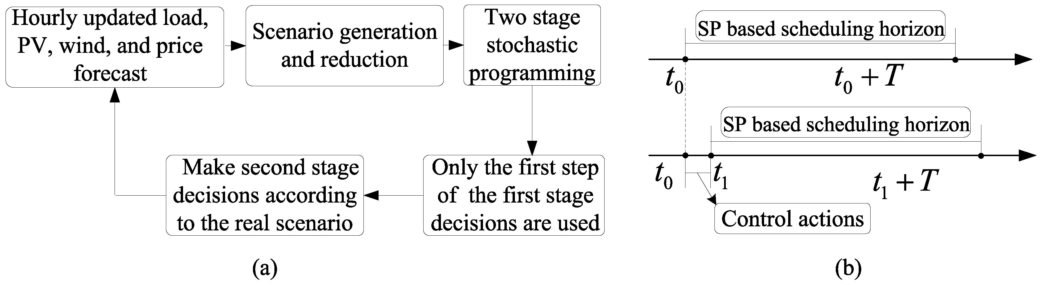
4. Receding Horizon Control

The buffering effect of battery storage system in the MG makes the state transitions over the entire time horizon of MG energy management, which increases the computational complexity. The charging/discharging schedule strategy of battery storage system and the unit commitment of DGs are associated with the MG operating cost. Furthermore, the forecast errors of load demand, PV and wind power production, and electricity price have great influence on the scheduling strategy. Because of the forecast errors increasing as the forecasting time horizons become longer, the SP based open loop strategy cannot deal with the forecast errors effectively without using the updated forecast information. In this paper, RHC strategy is proposed to be combine with the SP strategy. By using the lately updated forecast information, RHC can further compensate the uncertainty through a feedback mechanism.

The flowchart of SPRHC based MG energy management and the receding horizon procedure are shown in Figure 2. The basic idea of RHC is to calculate the optimal control sequences yet implement only the first step of them and ignore the rest [37]. In other words, the two-stage SP problem as illustrated in Section 3 is solved and derives the control sequences of a certain scheduling horizon T ($d_t$, $d_{t+1}$,…,$d_T$, where $d_t$ denotes the decision at time interval t), yet only the first time step of the control actions, i.e., $d_t$, are implemented.

As shown in Figure 2, at each time step t, the load demand, PV and wind production, and electricity price forecasts are updated. Based on the forecast information, several possible scenarios are derived through scenario generation and reduction strategy. According to the reduced set of scenarios, the two-stage SP problem as illustrated in Section 3 is solved and derives the control sequences of a certain scheduling horizon, yet only the first time step of the control actions are implemented in the first stage. Then, the second stage control actions at time interval t are made according to the first stage decisions and the particular realization of the real scenario. The system response to the control actions at time interval t will be measured as the next available information for solving the two-stage SP problem in the next interval. In the next time interval $t+1$, the system information (e.g., the load demand, PV and wind production, and electricity price forecasts) is updated and the two-stage SP problem is resolved. By implementing these steps with an RHC strategy, the feedback mechanism can further compensate the uncertainty in MG.

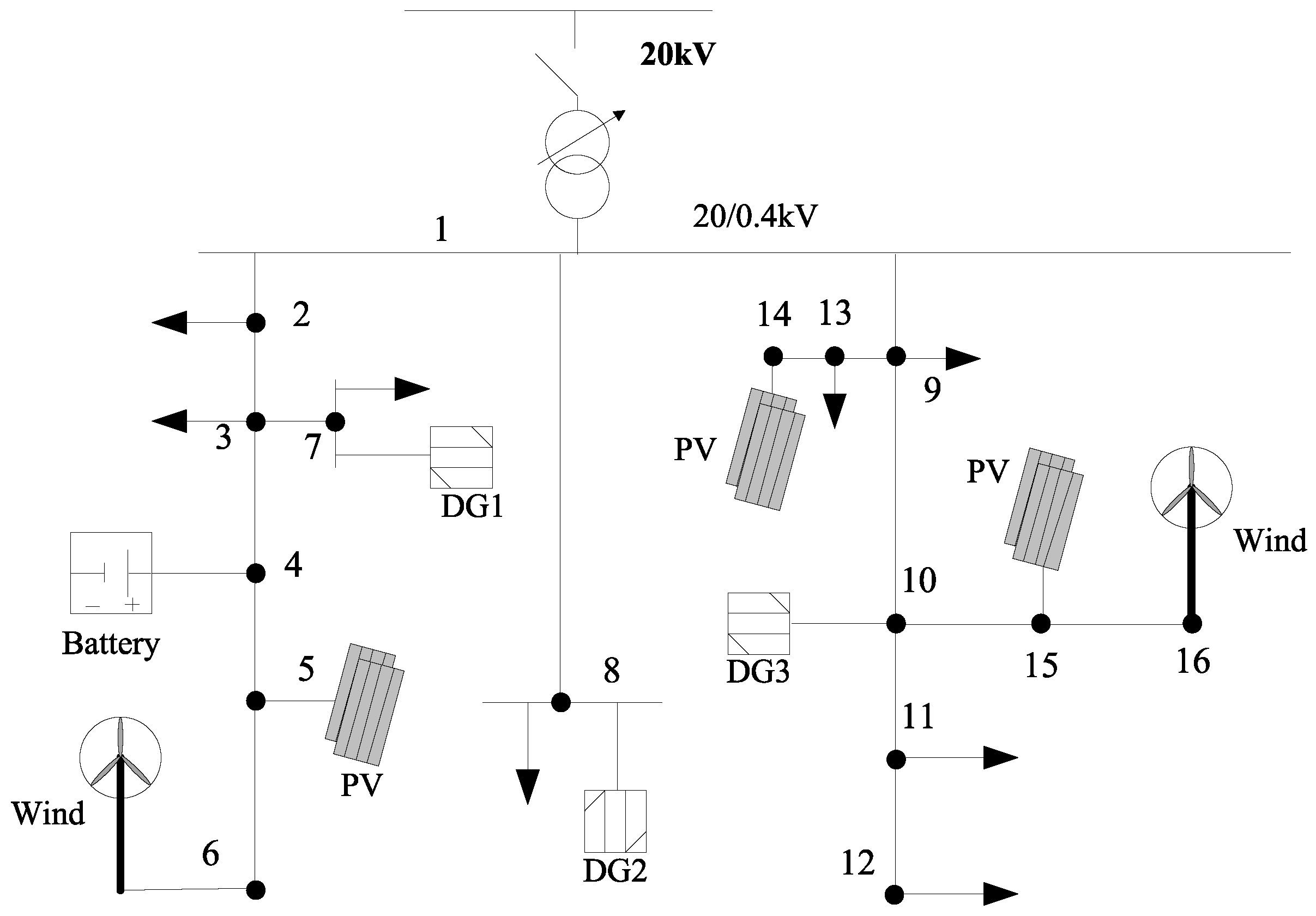
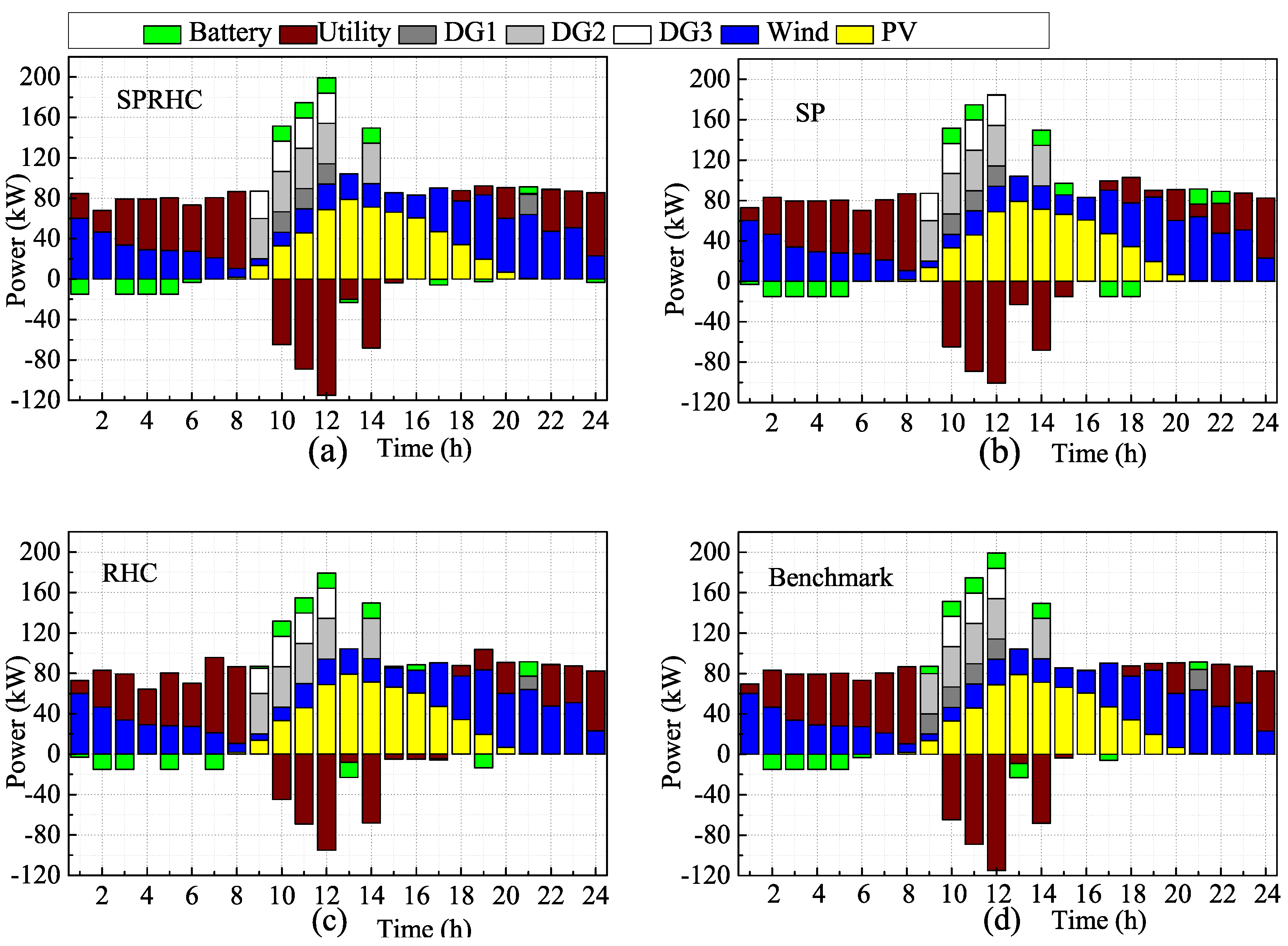
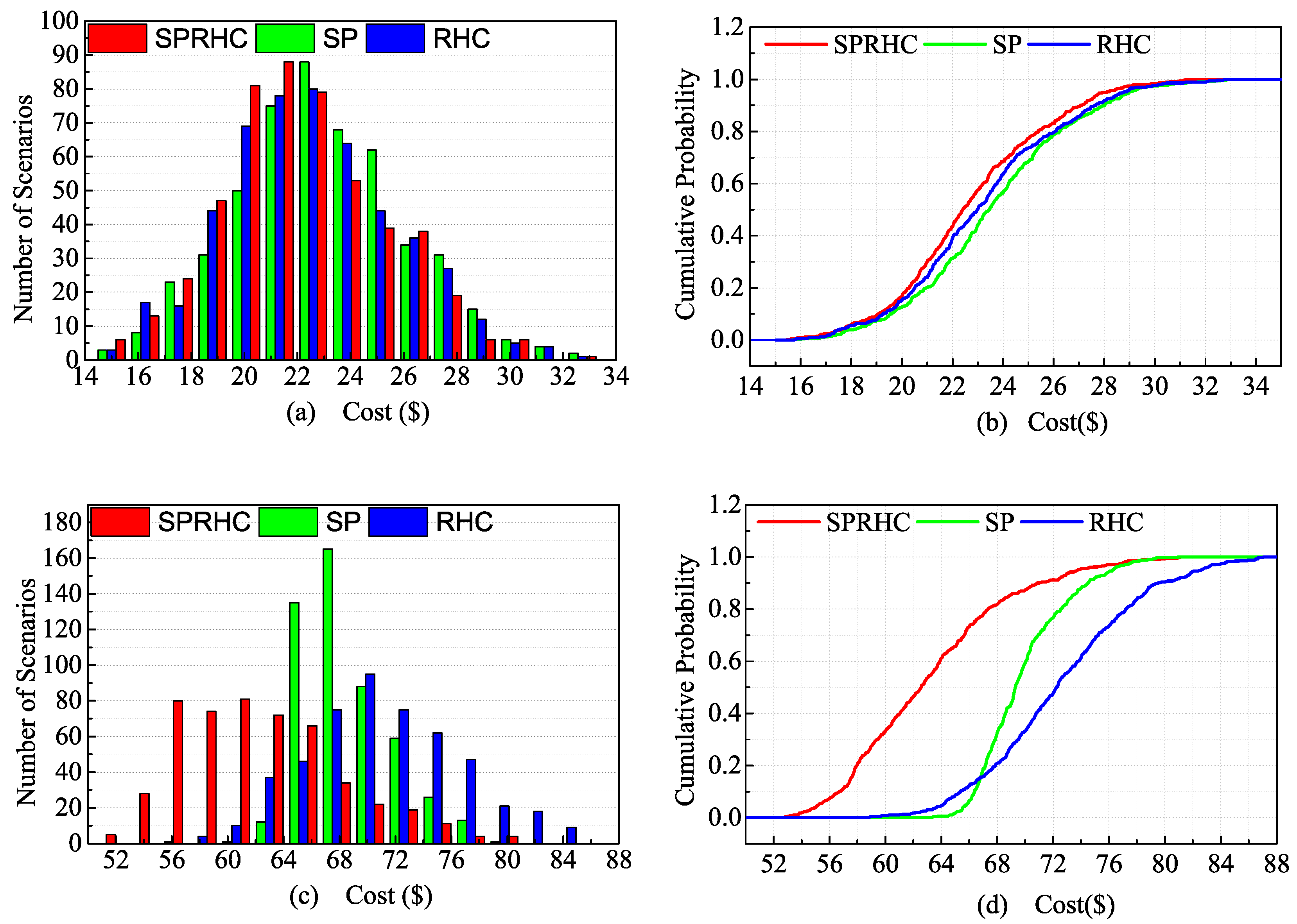
5. Numerical Experiments

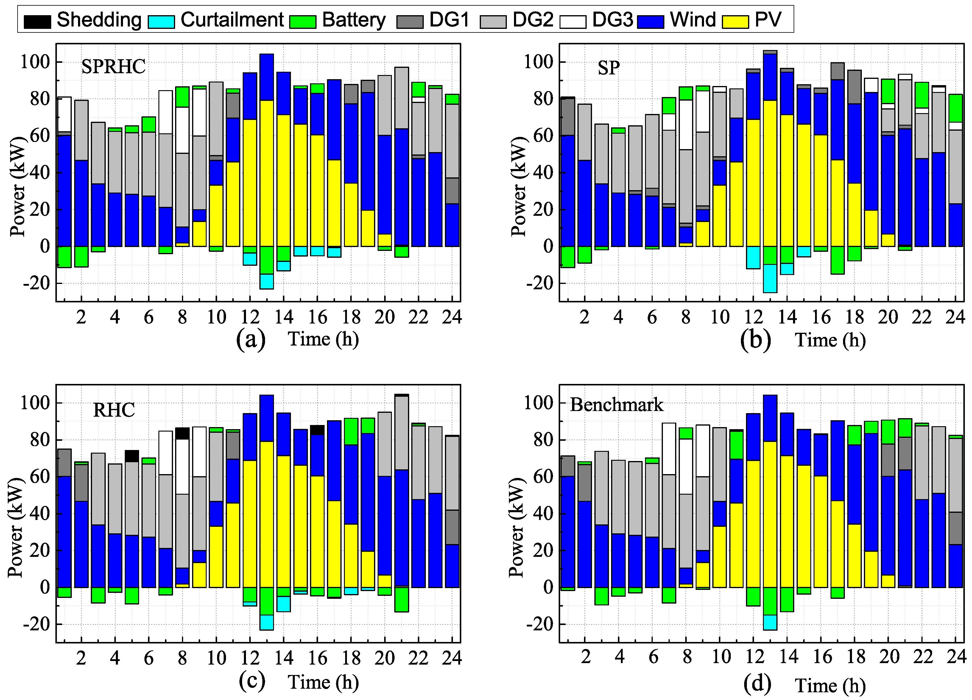
In this paper, a typical low voltage MG [38] is used to verify the effectiveness of the proposed SPRHC scheduling strategy for MG energy management under uncertainty. The test MG system consists of three PV generators, two wind generators, three controllable distributed generators (DGs), and one battery storage system, as shown in Figure 3. The forecast and real aggregated power production curves of PV and Wind as well as the load demand are collected and modified from Elia [39]. The degradation cost of battery (i.e., $Pric{e}^{Bat}$) are collected from [6]. In order to reduce the negative impacts of the uncertainty in MG to the external macro-grid, the selling price (i.e., $Pric{e}_{t,s}^{export}$) is always set lower than purchasing price to incite local use of PV and wind power [40]. In this paper, the price of exported power to the utility (i.e., $Pric{e}_{t,s}^{export}$) is assumed to be 0.2 multiplied by the purchasing price (i.e., $Pric{e}_{t,s}^{import}$). The normalized standard deviations (i.e., ${\mathsf{\delta }}^{PV},{\mathsf{\delta }}^{Wind},{\mathsf{\delta }}^{Load},{\mathsf{\delta }}^{Price}$) of forecast errors for PV, wind, load, and electricity price are collected and modified from [26,27,30,41]. All the data used for simulation is shown in

Table 1. Data used for simulation.

Symbol	Values
${\mathsf{\delta }}_1^{PV}$, ${\mathsf{\delta }}_1^{Wind}$, ${\mathsf{\delta }}_1^{Load}$, ${\mathsf{\delta }}_1^{Price}$	1.5%, 5%, 0.8%, 2%
${\mathsf{\delta }}_T^{PV}$, ${\mathsf{\delta }}_T^{Wind}$, ${\mathsf{\delta }}_T^{Load}$, ${\mathsf{\delta }}_T^{Price}$	7%, 35%, 4.5%, 9%
$Pric{e}^{Bat}$	0.0135 ($/kWh)
$Pric{e}^{Shed}$	0.5 ($/kWh)
$Pric{e}^{Curt}$	0.01 ($/kWh)
$P_1^{DGmin}$, $P_1^{DG max}$	2 (kW), 20 (kW)
$P_2^{DGmin}$, $P_2^{DG max}$	4 (kW), 40 (kW)
$P_3^{DGmin}$, $P_3^{DG max}$	3 (kW), 30 (kW)
$So{c}^{min}$, $So{c}^{max}$	15 (kWh), 75 (kWh)
$P^{Bat max}$,	15 (kW)
$S{U}_1^{DG}$, $S{D}_1^{DG}$	0.11 ($), 0.11 ($)
$S{U}_2^{DG}$, $S{D}_2^{DG}$	0.2 ($), 0.2 ($)
$S{U}_3^{DG}$, $S{D}_1^{DG}$	0.2 ($), 0.2 ($)
$a_1$, $b_1$, $c_1$	0.00011 ($/$\text{k}{\text{W}}^2\text{h}$), 0.0583 ($/kWh), 0.52 ($/h)
$a_2$, $b_2$, $c_2$	0.00011 ($/$\text{k}{\text{W}}^2\text{h}$), 0.034 ($/kWh), 1.47 ($/h)
$a_3$, $b_3$, $c_3$	0.00011 ($/$\text{k}{\text{W}}^2\text{h}$), 0.046 ($/kWh), 1.00 ($/h)
${\mathsf{\eta }}^c$, ${\mathsf{\eta }}^d$	0.95, 0.95

DG: distributed generator; SU: start-up; SD: shut-down.

.

The simulations were run on a PC with Intel(R) Core(TM) i7-2600 CPU @3.40GHz and 4.00 GB memory. The IBM ILOG CPLEX v12.60 optimization solver is utilized for solving the MICQP model. MATLAB 2015b and the YALMIP toolbox [42] are used for linking the CPLEX solver and computing the model.

In order to capture complete cycles of the load, solar, wind and electricity price profiles, the problem is investigated in 24 h horizon with 1 h time resolution in this paper. As described in Section 2, the scenario generation methodology was firstly implemented to create 500 scenarios for 24 h ahead with hourly resolution. Then, the created equiprobable scenarios were reduced to 10 scenarios using the scenario reduction algorithm outlined in Section 2. Figure 4, Figure 5, Figure 6 and Figure 7 illustrates the generated 500 equiprobable scenarios for 24 h ahead and the final reduced set of 10 scenarios by applying the BRA algorithm on the original 500 scenarios of imported electricity price, load, PV and wind, respectively. As shown in Figure 4, Figure 5, Figure 6 and Figure 7, one can observe that the prediction errors increased as the forecasting time horizons become longer.

In order to analyze the superiority of the proposed SPRHC strategy, the following strategies are implemented for the MG in both grid-connected operating mode and island operating mode:

(1)

SPRHC: the 24 h horizon power schedule was obtained by solving the two-stage stochastic programming problem described in Section 3 with the proposed SPRHC strategy.

(2)

SP: the 24 h horizon power schedule was obtained by solving the two-stage stochastic programming problem described in Section 3 with only an SP strategy.

(3)

RHC: the 24 h horizon power schedule was obtained by solving the optimization problem with only RHC strategy based on forecasted values of load demand, PV and wind power production, and electricity price, without considering the forecast errors.

(4)

Benchmark: the 24 h horizon power schedule was obtained by solving the optimization problem with perfect forecast, it assumes that the operator knows all the future realizations of the uncertainty in PV, wind, load, and electricity price.

Figure 8 shows the comparison of 24 h horizon power schedule obtained through SPRHC, SP, RHC, and Benchmark strategies when the MG is in grid-connected mode. For the power schedule shown in Figure 8d, it is optimal as the operator is assumed to know the perfect information. As shown in Figure 8d, the battery is charged during the 2nd–6th, 13th, and 17th time intervals, as the price is lower, while it is discharged during the 9th–12th, 14th, and 21st time intervals, as the price is higher during those time intervals. During the 10th–12th time intervals, all three DGs are turned on and output the maximum power to sell to the utility, as the price is higher during this period. However, only DG2 is turned on during the 14th time interval (the price is also very high), because the high price is sustained for only one time interval, and only DG2 can cover the on/off cost for selling the power to the utility. During the 9th time interval, DG1 and DG2 are turned on to compensate the load demand, and during the 21st time interval, only DG1 is turned on to compensate the load demand. During the other time intervals, the power demand is compensated by the utility, as the price is lower during those time intervals. As shown in Figure 8a–d, the power schedule obtained through the SPRHC strategy is more similar to the Benchmark than that obtained through SP and RHC strategies. The reason is as follows: although the SP strategy can provide a scheduling plan that minimizes the risk from the impact of uncertainty, it did not use the lately updated forecast information through an RHC mechanism, while the RHC strategy did not consider the forecast errors, which will have a higher risk from the impact of inaccurate forecasts; the SPRHC strategy considered the forecast errors through SP and involved a feedback mechanism through RHC by using the lately updated forecast information, which can effectively avoid short sighting and further compensate the uncertainty.

Figure 9 shows the comparison of a 24 h horizon power schedule obtained through SPRHC, SP, RHC, and Benchmark strategies when the MG is in island mode. The power schedule obtained through the Benchmark strategy is also optimal. As shown in Figure 9d, the battery is charged when the load demand is low and the PV and wind power production is high, while it is discharged when the load is high and the PV and wind power production is low. The unit commitment of DGs is also optimal, which is decided according to the generation cost coefficients, load demand, PV and wind production curves. Similar to the power schedule in grid-connected mode, the power schedule obtained through SPRHC strategy is also more similar to the Benchmark than that obtained through SP and RHC strategies, as can be seen from Figure 9a–d.

In order to evaluate the performance of the generated power schedules obtained through SPRHC, SP, and RHC strategies shown in Figure 8 and Figure 9, the power schedules are fed into 500 possible random scenarios that are regenerated with the scenario generation strategy shown in Section 2. In order to make a fair comparison, the simulations for the SPRHC, SP and RHC consider the same set of scenarios. The statistics of MG total operating cost with SP, RHC and SPRHC strategies are shown in

Table 2. Statistic of microgrid (MG) total operating cost with stochastic programming (SP), recording horizon control (RHC) and combined stochastic programming and recording horizon control (SPRHC) strategies.

Mode		SP	RHC	SPRHC
Grid-connect	average	23.6052	23.1895	22.7472
	min	15.6924	15.7484	15.4576
	max	33.2349	33.6729	33.3395
island	average	69.8766	72.5388	63.1397
	min	62.7694	57.4909	51.3237
	max	80.8760	86.9729	81.0506

. Both the comparison of the approximated probability distribution function (PDF) and cumulative distribution function (CDF) of MG total operating cost with SPRHC, SP and RHC strategies are illustrated in Figure 10.

As shown in Figure 10a,b, the operating cost when the MG is in island mode is higher than when it is in grid-connected mode. Because the uncertainty can be compensated by the utility when the MG is in grid-connected mode, while in island mode, the uncertainty in the MG can only be compensated by the high cost of DGs or load shedding. As shown in Table 2, the maximum costs of the SP strategy is a little lower than that of the SPRHC strategy. The SP procedure seems to be more effective to avoid scenarios where the costs can be very high. However, as shown in Figure 10, the probability of scenarios where the costs can be very high is very small. Thus, the proposed SPRHC strategy is more economic than both the SP and RHC strategies in the long term.

6. Conclusions

In this paper, an SPRHC strategy is presented for microgrid energy management under uncertainty. The uncertainties of RES, load, and electricity price are involved in the MG SPRHC optimization model. MCS based scenario generation and BRA based scenario reduction strategies are applied to transfer the complicated SP problem to a deterministic optimization problem. Furthermore, in the scenario generation and reduction process, the rate of forecast errors increased as the forecasting time horizons becoming longer was taken into account. The comparison results of the MG total operating cost with SPRHC, SP and RHC strategies demonstrate the superiority of the proposed strategy for both island and grid-connected operating modes of an MG.

References

1. Marnay, C.; Chatzivasileiadis, S.; Abbey, C.; Iravani, R.; Joos, G.; Lombardi, P.; Mancarella, P.; von Appen, J. Microgrid Evolution Roadmap. In Proceedings of the 2015 International Symposium on Smart Electric Distribution Systems and Technologies (EDST), Vienna, Austria, 8–11 September 2015; pp. 139–144.
2. Wang, R.; Wang, P.; Xiao, G. A robust optimization approach for energy generation scheduling in microgrids. Energy Convers. Manag. 2015, 106, 597–607. [Google Scholar] [CrossRef]
3. Kuznetsova, E.; Li, Y.F.; Ruiz, C.; Zio, E. An integrated framework of agent-based modelling and robust optimization for microgrid energy management. Appl. Energy 2014, 129, 70–88. [Google Scholar] [CrossRef]
4. Bertsimas, D.; Litvinov, E.; Sun, X.A.; Zhao, J.; Zheng, T. Adaptive Robust Optimization for the Security Constrained Unit Commitment Problem. IEEE Trans. Power Syst. 2013, 28, 52–63. [Google Scholar] [CrossRef]
5. Zhou, Z.; Zhang, J.; Liu, P.; Li, Z.; Georgiadis, M.C.; Pistikopoulos, E.N. A two-stage stochastic programming model for the optimal design of distributed energy systems. Appl. Energy 2013, 103, 135–144. [Google Scholar] [CrossRef]
6. Li, H.; Zang, C.; Zeng, P.; Yu, H.; Li, Z. A stochastic programming strategy in microgrid cyber physical energy system for energy optimal operation. IEEE/CAA J. Autom. Sin. 2015, 2, 296–303. [Google Scholar]
7. Zakariazadeh, A.; Jadid, S.; Siano, P. Smart microgrid energy and reserve scheduling with demand response using stochastic optimization. Int. J. Electr. Power Energy Syst. 2014, 63, 523–533. [Google Scholar] [CrossRef]
8. Niknam, T.; Azizipanah-Abarghooee, R.; Narimani, M.R. An efficient scenario-based stochastic programming framework for multi-objective optimal micro-grid operation. Appl. Energy 2012, 99, 455–470. [Google Scholar] [CrossRef]
9. Taylor, J.W.; De Menezes, L.M.; McSharry, P.E. A comparison of univariate methods for forecasting electricity demand up to a day ahead. Int. J. Forecast. 2006, 22, 1–16. [Google Scholar] [CrossRef] [Green Version]
10. Martin, L.; Zarzalejo, L.F.; Polo, J.; Navarro, A.; Marchante, R.; Cony, M. Prediction of global solar irradiance based on time series analysis: Application to solar thermal power plants energy production planning. Sol. Energy 2010, 84, 1772–1781. [Google Scholar] [CrossRef]
11. Makarov, Y.V.; Etingov, P.V.; Ma, J.; Huang, Z.; Subbarao, K. Incorporating Uncertainty of Wind Power Generation Forecast Into Power System Operation, Dispatch, and Unit Commitment Procedures. IEEE Trans. Sustain. Energy 2011, 2, 433–442. [Google Scholar] [CrossRef]
12. Lange, M. On the uncertainty of wind power predictions - Analysis of the forecast accuracy and statistical distribution of errors. J. Sol. Energy Eng.-Trans. ASME 2005, 127, 177–184. [Google Scholar] [CrossRef]
13. Parisio, A.; Glielmo, L. Stochastic Model Predictive Control for economic/environmental operation management of microgrids. In Proceedings of the 2013 European Control Conference (ECC), Zurich, Switzerland, 17–19 July 2013; pp. 2014–2019.
14. Olivares, D.E.; Lara, J.D.; Canizares, C.A.; Kazerani, M. Stochastic-Predictive Energy Management System for Isolated Microgrids. IEEE Trans. Smart Grid 2015, 6, 2681–2693. [Google Scholar] [CrossRef]
15. Korpas, M.; Holen, A.T. Operation planning of hydrogen storage connected to wind power operating in a power market. IEEE Trans. Energy Convers. 2006, 21, 742–749. [Google Scholar] [CrossRef]
16. Kriett, P.O.; Salani, M. Optimal control of a residential microgrid. Energy 2012, 42, 321–330. [Google Scholar] [CrossRef]
17. Zhang, Y.; Liu, B.; Zhang, T.; Guo, B. An Intelligent Control Strategy of Battery Energy Storage System for Microgrid Energy Management under Forecast Uncertainties. Int. J. Electrochem. Sci. 2014, 9, 4190–4204. [Google Scholar]
18. Prodan, I.; Zio, E. A model predictive control framework for reliable microgrid energy management. Int. J. Electr. Power Energy Syst. 2014, 61, 399–409. [Google Scholar] [CrossRef]
19. Su, W.; Wang, J.; Zhang, K.; Huang, A.Q. Model predictive control-based power dispatch for distribution system considering plug-in electric vehicle uncertainty. Electr. Power Syst. Res. 2014, 106, 29–35. [Google Scholar] [CrossRef]
20. Gröwe-Kuska, N.; Heitsch, H.; Römisch, W. Scenario reduction and scenario tree construction for power management problems. In Proceedings of the 2003 IEEE Bologna Power Tech Conference Proceedings, Bologna, Italy, 23–26 June 2003; Volume 3.
21. Mathiesen, P.; Kleissl, J. Evaluation of numerical weather prediction for intra-day solar forecasting in the continental United States. Sol. Energy 2011, 85, 967–977. [Google Scholar] [CrossRef]
22. Manda, P.; Senjyu, T.; Naomitsu, U.; Funabashi, T. A neural network based several-hour-ahead electric load forecasting using similar days approach. Int. J. Electr. Power Energy Syst. 2006, 28, 367–373. [Google Scholar] [CrossRef]
23. Foley, A.M.; Leahy, P.G.; Marvuglia, A.; McKeogh, E.J. Current methods and advances in forecasting of wind power generation. Renew. Energy 2012, 37, 1–8. [Google Scholar] [CrossRef] [Green Version]
24. Li, Z.; Zang, C.; Zeng, P.; Yu, H.; Li, H. Day-ahead hourly photovoltaic generation forecasting using extreme learning machine. In Proceedings of the 2015 IEEE International Conference on Cyber Technology in Automation, Control, and Intelligent Systems (CYBER), Shenyang, China, 8–12 June 2015; pp. 779–783.
25. Dong, Y.; Wang, J.; Jiang, H.; Wu, J. Short-term electricity price forecast based on the improved hybrid model. Energy Convers. Manag. 2011, 52, 2987–2995. [Google Scholar] [CrossRef]
26. Aggarwal, S.K.; Saini, L.M.; Kumar, A. Electricity price forecasting in deregulated markets: A review and evaluation. Int. J. Electr. Power Energy Syst. 2009, 31, 13–22. [Google Scholar] [CrossRef]
27. Vagropoulos, S.I.; Kardakos, E.G.; Simoglou, C.K.; Bakirtzis, A.G.; Catalao, J.P.S. ANN-based scenario generation methodology for stochastic variables of electric power systems. Electr. Power Syst. Res. 2016, 134, 9–18. [Google Scholar] [CrossRef]
28. Holjevac, N.; Capuder, T.; Kuzle, I. Adaptive control for evaluation of flexibility benefits in microgrid systems. Energy 2015, 92, 487–504. [Google Scholar] [CrossRef]
29. Alabedin, A.M.Z.; El-Saadany, E.F.; Salama, M.M.A. Generation scheduling in Microgrids under uncertainties in power generation. In Proceedings of the 2012 IEEE Electrical Power and Energy Conference (EPEC), London, ON, Canada, 10–12 October 2012; pp. 133–138.
30. Ding, Z. Optimal Operation Of Microgrid under a Stochastic Environment. Ph.D. Thesis, The University of Texas at Arlington, Arlington, TX, USA, 2015. [Google Scholar]
31. Rezaei, N.; Kalantar, M. A novel hierarchical energy management of a renewable microgrid considering static and dynamic frequency. J. Renew. Sustain. Energy 2015, 7. [Google Scholar] [CrossRef]
32. Liu, P.; Fu, Y.; Marvasti, A.K. Multi-stage Stochastic Optimal Operation of Energy-efficient Building with Combined Heat and Power System. Electr. Power Compon. Syst. 2014, 42, 327–338. [Google Scholar] [CrossRef]
33. Zanjani, M.K.; Nourelfath, M.; Ait-Kadi, D. A multi-stage stochastic programming approach for production planning with uncertainty in the quality of raw materials and demand. Int. J. Product. Res. 2010, 48, 4701–4723. [Google Scholar] [CrossRef]
34. Lucia, S.; Engell, S. Multi-stage and two-stage robust nonlinear model predictive control. In Proceedings of the Nonlinear Model Predictive Control, Leeuwenhorst, The Netherlands, 23–27 August 2012; Volume 4, pp. 181–186.
35. Xu, Y.; Zhang, W.; Liu, W. Distributed Dynamic Programming-Based Approach for Economic Dispatch in Smart Grids. IEEE Trans. Ind. Inform. 2015, 11, 166–175. [Google Scholar] [CrossRef]
36. Almassalkhi, M.R.; Hiskens, I.A. Model-Predictive Cascade Mitigation in Electric Power Systems with Storage and Renewables-Part I: Theory and Implementation. IEEE Trans. Power Syst. 2015, 30, 67–77. [Google Scholar] [CrossRef]
37. Wang, R.; Wang, P.; Xiao, G.; Gong, S. Power demand and supply management in microgrids with uncertainties of renewable energies. Int. J. Electr. Power Energy Syst. 2014, 63, 260–269. [Google Scholar] [CrossRef]
38. Tsikalakis, A.G.; Hatziargyriou, N.D. Centralized Control for Optimizing Microgrids Operation. IEEE Trans. Energy Convers. 2008, 23, 241–248. [Google Scholar] [CrossRef]
39. Belgiums Electricity Transmission System Operator Website. 2014. Available online: http://www.elia.be (accessed on 30 April 2016).
40. Zhang, Y.; Zhang, T.; Wang, R.; Liu, Y.; Guo, B. Optimal operation of a smart residential microgrid based on model predictive control by considering uncertainties and storage impacts. Sol. Energy 2015, 122, 1052–1065. [Google Scholar] [CrossRef]
41. Castronuovo, E.; Lopes, J. On the optimization of the daily operation of a wind-hydro power plant. IEEE Trans. Power Syst. 2004, 19, 1599–1606. [Google Scholar] [CrossRef]
42. Lofberg, J. YALMIP: A toolbox for modeling and optimization in MATLAB. In Proceedings of the 2004 IEEE International Symposium on Computer Aided Control Systems Design, Taipei, Taiwan, 4 September 2004; pp. 284–289.
Figure 1. Diagram of a backward reduction algorithm (BRA) algorithm.
Energies 09 00499 g001
Figure 2. Scheme of combined stochastic programming and receding horizon control (SPRHC) based microgrid (MG) energy management (a) flowchart of SPRHC (b) receding horizon procedure.
Energies 09 00499 g002
Figure 3. The low voltage MG for case study.
Energies 09 00499 g003
Figure 4. Scenario generation and reduction of price profile for imported power from the utility (a) generated 500 imported electricity price scenarios for 24 h ahead with increasing standard deviation; (b) reduced set of 10 final scenarios by applying the BRA algorithm to the original 500 scenarios.
Energies 09 00499 g004
Figure 5. Scenario generation and reduction of aggregated load demand (a) generated 500 load scenarios for 24 h ahead with increasing standard deviation; (b) reduced set of 10 final scenarios by applying the BRA algorithm on the original 500 scenarios.
Energies 09 00499 g005
Figure 6. Scenario generation and reduction of aggregated photovoltaic (PV) power production (a) generated 500 PV scenarios for 24 h ahead with increasing standard deviation; (b) reduced set of 10 final scenarios by applying the BRA algorithm to the original 500 scenarios.
Energies 09 00499 g006
Figure 7. Scenario generation and reduction of aggregated wind power production (a) generated 500 wind scenarios for 24 h ahead with increasing standard deviation; (b) reduced set of 10 final scenarios by applying the BRA algorithm to the original 500 scenarios.
Energies 09 00499 g007
Figure 8. Power schedule in grid-connected mode (a) SPRHC strategy; (b) SP strategy; (c) RHC strategy; (d) Benchmark.
Energies 09 00499 g008
Figure 9. Power schedule in island mode (a) SPRHC strategy; (b) SP strategy; (c) RHC strategy; (d) Benchmark.
Energies 09 00499 g009
Figure 10. Probability distribution function (PDF) and cumulative distribution function (CDF) of MG total operating cost with SP, RHC and SPHC strategy (a) PDF in grid-connected mode; (b) CDF in grid-connected mode; (c) PDF in island mode; (d) CDF in island mode.
Energies 09 00499 g010