Optimal Operation of Network-Connected Combined Heat and Powers for Customer Profit Maximization

Abstract

Network-connected combined heat and powers (CHPs), owned by a community, can export surplus heat and electricity to corresponding heat and electric networks after community loads are satisfied. This paper proposes a new optimization model for network-connected CHP operation. Both CHPs’ overall efficiency and heat to electricity ratio (HTER) are assumed to vary with loading levels. Based on different energy flow scenarios where heat and electricity are exported to the network from the community or imported, four profit models are established accordingly. They reflect the different relationships between CHP energy supply and community load demand across time. A discrete optimization model is then developed to maximize the profit for the community. The models are derived from the intervals determined by the daily operation modes of CHP and real-time buying and selling prices of heat, electricity and natural gas. By demonstrating the proposed models on a 1 MW network-connected CHP, results show that the community profits are maximized in energy markets. Thus, the proposed optimization approach can help customers to devise optimal CHP operating strategies for maximizing benefits.

1. Introduction

With the depletion of fossil fuel and increasingly severe global warming issues, renewable energy sources and high-efficiency energy consumption technologies are attracting wide interest [1]. Traditionally, heat and electricity are provided with boilers and thermal power plants separately, whose overall efficiency is very low [2]. The low energy utilization efficiency means a waste of resources and a large amount of greenhouse gas emissions particularly carbon dioxide [3]. The existing problems provide incentives to utilize energy more efficiently.

The combined heat and power (CHP) system is a very promising technology in reducing fuel cost and greenhouse gases emission [4,5,6,7]. A CHP system is able to produce heat and electricity in a single process from oil or natural gas at an efficiency of over 80% compared to an average of 30%–35% for conventional thermal generation [8,9,10,11]. The extraction condensing steam turbine CHP is increasingly used in both industry and residency because the ratio between heat and electricity output of CHPs can be adjusted to satisfy different heat and electric demand [12,13,14,15].

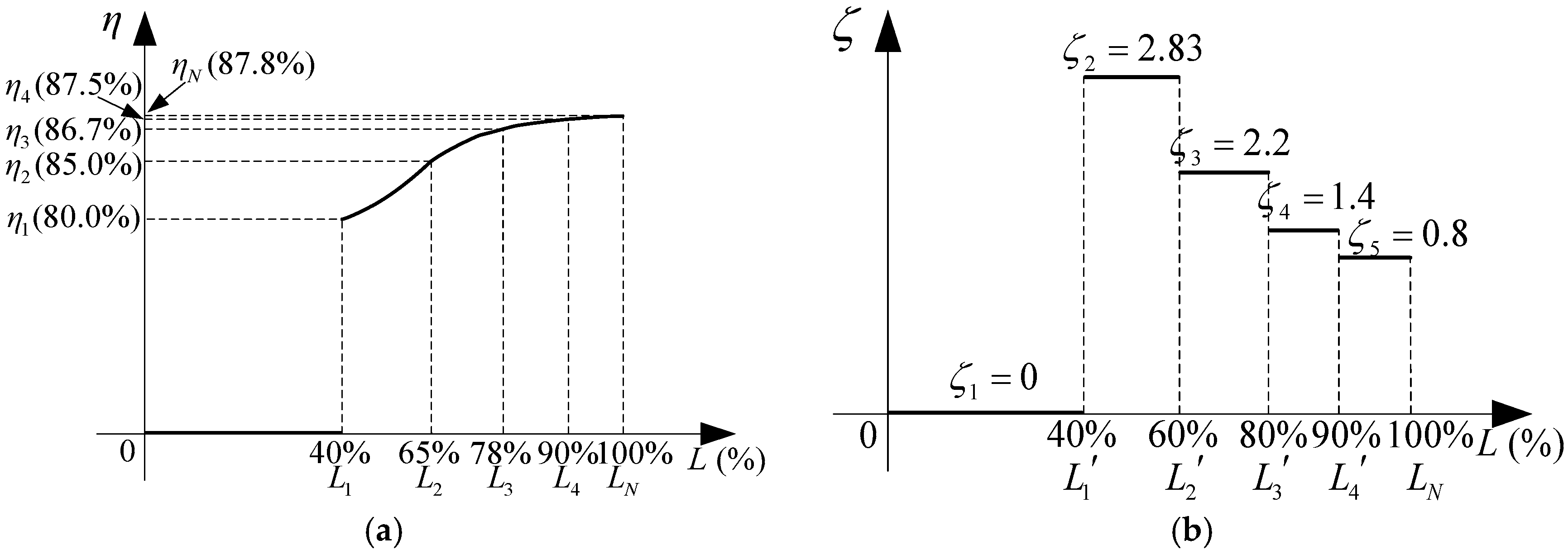
The output of CHP is driven by load demand [16,17]. Heat to electricity ratio (HTER) is introduced in this paper to characterize the heat and electricity output proportion of CHPs. When heat demand is high, the CHP is operated with the heat leading (HL) strategy to mainly satisfy heat load, and HTER is at a high value correspondingly. When electricity load is large, the CHP is operated with electricity leading (EL) strategy to supply electric load first, where HTER is at a low level [18]. During valley hours, the output of CHP has to be decreased.

In most research, the heat and electricity output of CHPs is only to meet the demand of residential, commercial or industrial users, which are called isolated CHPs in this paper. For isolated CHPs, they only produce heat and electricity for customers and have no interactions with heat and electricity networks. In [19], the domestic energy cost savings of isolated CHPs are investigated with demand response based on the proposed model-predictive control strategy. Results show that the energy cost reduces dramatically in the real-time market. The authors in [20] construct environmental impact models for a traditional separation production and isolated combined cooling heat and powers (CCHPs), respectively, to analyze their energy consumption. The energy savings and emission reductions are maximized when the capacity of the CCHP system is optimized by a genetic algorithm. A multi-objective optimization model, including technical, economic, energetic and environmental indicators, is developed in [21] for the design of CHP plants in realistic conditions. The main drawback of the above research is that CHP is optimized in either EL or HL strategies, and they also neglect that HTER varies with the overall efficiency and loading level of CHPs [22].

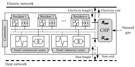
To achieve energy consumption in a more efficient way, different energy carrier networks are connected together [23]. Then, network-connected CHPs are the core of such an energy system, which are connected to heat and electric networks. Surplus heat and electricity are exported to corresponding heat and electricity networks after the load in the community is satisfied. The matching analysis is conducted in [24] to access the capability of CHP from electrical grid feed-in and heat grid feed-in strategies, respectively. Results show that the matching results have no linear relation with the energy consumption. Reference [25] is focused on reducing the operational cost of a CHP-based microgrid through multi-objective self-scheduling optimization. A techno-economic model for CHP is developed in [26] based on dynamic economics, and the heating cost of the system is reduced to the least with the application of CHP in regulating peak load. Aforementioned literature is mainly concentrated on the least operation cost or least emissions, which does not necessarily mean high profit.

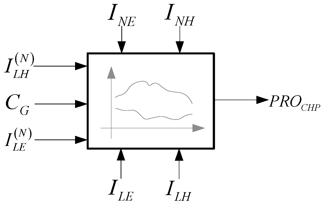
In this paper, the network-connected CHPs owned by the community have the characteristics that both overall efficiency and HTER vary with the system loading level. After the demand in the community is satisfied, surplus heat and electricity are sold to the heat and electricity networks. Then, based on the relationship between community heat and electric demand and CHP output, four operation modes are obtained. Finally, a discrete optimization model is derived, which is determined by the price intervals (30 min) and operation modes of CHP together. After demonstrating the proposed model on a 1 MW network-connected CHP, both energy purchasing costs and profits are optimized. Results show the profit is maximized during valley hours, and the cost of buying additional energy is minimized during peak hours.

The novelty of this paper is that it: (i) proposes a network-connected CHP model with time-varying bi-directional energy flow between itself and networks; (ii) constructs the profit models for network-connected CHPs under different load conditions; and (iii) proposes a discrete optimization strategy to maximize profit in real time.

The remaining parts of this paper are organized as follows: in Section 2, the model of a network-connected CHP is presented; the profit model for the CHP is established in Section 3, followed by the discrete optimization model in real time; in Section 4, a 1 MW CHP is optimized with the proposed models; finally, conclusions are drawn in Section 5.

2. Modelling of Network-Connected Combined Heat and Power

2.1. Schematic Diagram of Network-Connected Combined Heat and Power System

For a network-connected CHP system, it is connected to the heat and electricity networks simultaneously. A conceptual schematic diagram is shown in Figure 1. The CHP is installed in a community, which consists of n resident households, a small commercial center, and a small industrial center. The electric and heat energy produced by the CHP are denoted by E_CHP and H_CHP, respectively.

The heat and electric load in the community are satisfied either by the CHP or by energy imported from corresponding networks. The output of the CHP also flows in two directions, supplying community load or exporting to the heat and electric networks. During valley load periods, when heat and electric load in the community are at a low level, one of the two loads or both of them can be easily satisfied by the CHP. Then, the surplus energy is sold to corresponding networks. During peak load periods, the CHP may not be able to meet the high load demand in the community, and thus additional heat and electricity have to be imported from the networks. To evaluate the total profit of the CHP, its model should be established first.

2.2. Technical Model of Combined Heat and Power

According to the basic diagram of CHP in [27], the output of a CHP mainly includes four parts: heat, electricity, unavoidable heat loss and exhaust gas emissions. There are two key parameters used to model CHP: overall efficiency and HTER. The overall efficiency is to evaluate the ability of CHP to convert the gas energy to heat and electricity, denoted by η. HTER is the ratio of the heat output to the electricity output, denoted by ζ. The two parameters are expressed by:

$$\{\begin{array}{l}\mathsf{\eta }=\frac{Q_{\mathrm{U}}}{G_{\mathrm{I}\mathrm{N}}}\hfill \\ \mathsf{\zeta }=\frac{H_{\mathrm{CHP}}}{E_{\mathrm{CHP}}}\hfill \\ Q_{\mathrm{U}}=H_{\mathrm{CHP}}+E_{\mathrm{CHP}}\hfill \end{array}$$

(1)

where η is the overall energy efficiency of a CHP; Q_U is the sum of heat and electricity produced by a CHP, in kJ; G_IN is the energy of input natural gas, in kJ; H_CHP and E_CHP are the heat and electricity output of the CHP, respectively, both in kJ.

Usually, the energy contained in a base unit (a cubic meter) of natural gas is a constant, denoted by q, in kJ/m³. Thus, the total energy injected into the CHP can be expressed as:

$$G_{\mathrm{IN}}=q{V}_{\mathrm{G}}$$

(2)

where V_G is the volume of natural gas consumed by the CHP.

According to the research in [28,29], both η and ζ are highly relevant to the operation modes of the CHP. They are both in variation with the CHP’s loading level. The typical curves of η and ζ are shown in Figure 2 according to [27], and they are both modeled as discrete functions of the loading level L to capture the generality.

The overall efficiency η in Figure 2a is expressed as:

$$\mathsf{\eta }=\{\begin{array}{lllll}{f}_1\left(L\right)=0\hfill & \hfill & \hfill & \hfill & 0\le L<L_1\hfill \\ f_2\left(L\right)\hfill & \hfill & \hfill & \hfill & L_1\le L<L_2\hfill \\ f_3\left(L\right)\hfill & \hfill & \hfill & \hfill & L_2\le L<L_3\hfill \\ f_4\left(L\right)\hfill & \hfill & \hfill & \hfill & L_3\le L<L_4\hfill \\ f_5\left(L\right)\hfill & \hfill & \hfill & \hfill & L_4\le L\le L_N\hfill \end{array}$$

(3)

The typical values of the variables in Figure 2 are shown in

Table A1. Efficiency and HTER of CHP.

Typical Overall Efficiency		Loading Level	HTER		Loading Level
η1	80%	40%	ζ1	0	0%–40%
η2	85%	65%	ζ2	2.83	40%–60%
η3	86.7%	78%	ζ3	2.2	60%–80%
η4	87.5%	90%	ζ4	1.4	80%–90%
ηN	87.8%	100%	ζ5	0.8	90%-100%

in the Appendix. By substituting Equation (2) into Equation (1), the output of the CHP can also be expressed as:

$$\{\begin{array}{c}{E}_{\mathrm{CHP}}=\frac{q}{1+\mathsf{\zeta }}\mathsf{\eta }{V}_{\mathrm{G}}\\ H_{\mathrm{CHP}}=\frac{\mathsf{\zeta }q}{1+\mathsf{\zeta }}\mathsf{\eta }{V}_{\mathrm{G}}\end{array}$$

(4)

2.3. Profit Model for Combined Heat and Power

After taking the heat and electricity sold to networks into consideration, bi-directional energy flow between the network and community is possible. The corresponding energy prices, including that of heat and electricity bought from and sold to the network, will influence the profits of the community. The profit model of the community is shown in Figure 3.

In Figure 3, C_G is the fuel cost of CHP, which is mainly determined by the price and consumed volume of natural gas. The profit of the community is denoted by PRO_CHP. Equivalent heat income earned through consuming heat from CHP instead of heat network is denoted by I_LH. Similarly, the equivalent electric income earned through consuming electricity from CHP instead of importing from the network is denoted by I_LE. When the heat produced by CHP is larger than load demand during valley hours, the surplus heat is sold to the heat network and the corresponding income is denoted by I_NH. The surplus electricity is sold to the electric network, and the corresponding income is denoted by I_NE. During peak hours, the output of CHP is not able to supply the heat and electric demand. At this time, the heat and electricity deficit has to be bought from the heat and electric networks, respectively. The corresponding heat and electricity purchasing cost is denoted by $I_{\mathrm{LH}}^{\left(N\right)}$ and $I_{\mathrm{LE}}^{\left(N\right)}$, respectively. The total equivalent profit of the community can be expressed as follows:

$$PR{O}_{\mathrm{CHP}}=I_{\mathrm{LE}}+I_{\mathrm{LH}}+I_{\mathrm{NE}}+I_{\mathrm{NH}}-I_{\mathrm{LE}}^{\left(\mathrm{N}\right)}-I_{\mathrm{LH}}^{\left(\mathrm{N}\right)}-C_{\mathrm{G}}$$

(5)

In this research, the real-time prices of heat, electricity and natural gas are adopted. The income and cost in Equation (5) are calculated by:

$$\{\begin{array}{l}{I}_{\mathrm{LE}}=p_{\mathrm{LE}}{E}_{\mathrm{L},\mathrm{CHP}},I_{\mathrm{LH}}=p_{\mathrm{LH}}{H}_{\mathrm{L},\mathrm{CHP}}\hfill \\ I_{\mathrm{NE}}=p_{\mathrm{NE}}{E}_{\mathrm{N},\mathrm{CHP}},I_{\mathrm{NH}}=p_{\mathrm{NH}}{H}_{\mathrm{N},\mathrm{CHP}}\hfill \\ I_{\mathrm{LE}}^{\left(\mathrm{N}\right)}=p_{\mathrm{LE}}{E}_{\mathrm{L}}^{\left(\mathrm{N}\right)},I_{\mathrm{LH}}^{\left(\mathrm{N}\right)}=p_{\mathrm{LH}}{H}_{\mathrm{L}}^{\left(\mathrm{N}\right)}\hfill \\ C_{\mathrm{G}}=p_{\mathrm{G}}{V}_{\mathrm{G}}\hfill \end{array}$$

(6)

where p_LE and p_LH are the real-time prices of buying electricity and heat; p_G is the real-time price of natural gas; p_NE and p_NH are the real-time prices of selling electricity and heat to corresponding networks; E_L,CHP and H_L,CHP are the consumed electricity and heat energy in the community, which are supplied by CHP; E_N,CHP and H_N,CHP are the electricity and heat energy sold to the corresponding networks by the community; $E_{\mathrm{L}}^{\left(\mathrm{N}\right)}$ and $H_{\mathrm{L}}^{\left(\mathrm{N}\right)}$ are the bought electricity and heat from corresponding networks; and V_G is the consumed volume of natural gas.

The heat and electricity produced by CHP flow into two directions: consumed by the community or sold to the corresponding networks, which can be expressed as:

$$\{\begin{array}{c}{E}_{\mathrm{CHP}}=E_{\mathrm{L},\mathrm{CHP}}+E_{\mathrm{N},\mathrm{CHP}}\\ H_{\mathrm{CHP}}=H_{\mathrm{L},\mathrm{CHP}}+H_{\mathrm{N},\mathrm{CHP}}\end{array}$$

(7)

The consumed heat and electricity of the community come from two directions: supplied by CHP or bought from the corresponding networks, which can be expressed as:

$$\{\begin{array}{c}{E}_{\mathrm{L}}=E_{\mathrm{L},\mathrm{CHP}}+E_{\mathrm{L}}^{\left(\mathrm{N}\right)}\\ H_{\mathrm{L}}=H_{\mathrm{L},\mathrm{CHP}}+H_{\mathrm{L}}^{\left(\mathrm{N}\right)}\end{array}$$

(8)

where E_L and H_L are the electric and heat demand of the community, respectively.

3. Optimization Model of Combined Heat and Power

3.1. Profit Model for Different Operation Modes

Based on the relationship between E_CHP and E_L, and H_CHP and H_L, there are four operation modes for CHP. The main purpose of CHP is to satisfy the heat and electric demand of the community. Thus, surplus heat and electricity are sold to the networks only after E_L and H_L are satisfied. On the other hand, p_LE is usually higher than p_NE and p_LH is higher than p_NH. Thus, the special case is not considered where heat and electricity are sold to the networks when E_L and H_L are in deficit. After the above analysis, four operation modes for CHP are obtained, denoted by C₁, C₂, C₃ and C₄, respectively, shown in Figure 4.

In Figure 4, the dotted arrows mean that the energy flow does not exist in corresponding operation modes. The profits for the four operation modes are then calculated as follows.

3.1.1. C₁: P_E,CHP > P_E,L, P_H,CHP > P_H,L

Here, P_E,CHP and P_H,CHP are the output electricity and heat power of the CHP, both in kW. P_E,L and P_H,L are the electric and heat power demand of the community, both in kW. In Mode C₁ shown in Figure 4a, both the heat and electric load are in valley hours and satisfied by the CHP easily. At the same time, surplus heat and electricity are sold to the corresponding networks. Then, the energy supply and demand relation can be expressed as:

$$\{\begin{array}{l}{E}_{\mathrm{L},\mathrm{CHP}}=E_{\mathrm{L}},H_{\mathrm{L},\mathrm{CHP}}=H_{\mathrm{L}}\hfill \\ E_{\mathrm{L}}^{\left(\mathrm{N}\right)}=0,H_{\mathrm{L}}^{\left(\mathrm{N}\right)}=0\hfill \end{array}$$

(9)

By substituting Equations (6)–(9) into Equation (5), the profit for this mode is:

$$PR{O}_{\mathrm{CHP}}^{{\mathrm{C}}_1}=\left(p_{\mathrm{LE}}-p_{\mathrm{NE}}\right)E_{\mathrm{L}}+\left(p_{\mathrm{LH}}-p_{\mathrm{NH}}\right)H_{\mathrm{L}}+p_{\mathrm{NE}}{E}_{\mathrm{CHP}}+p_{\mathrm{NH}}{H}_{\mathrm{CHP}}-p_{\mathrm{G}}{V}_{\mathrm{G}}$$

(10)

where $PR{O}_{\mathrm{CHP}}^{{\mathrm{C}}_1}$ is the profit of the community in Mode C₁.

3.1.2. C₂: P_E,CHP > P_E,L, P_H,CHP < P_H,L

In Mode C₂, the electric demand is at a low level, while the heat is in great demand. The electric demand is supplied by the CHP, and the heat deficit has to be bought from the heat network. The case where additional electricity is bought from the electricity network does not exist in addition to the case where surplus heat is sold to the heat network, as the dotted arrows shown in Figure 4b. The energy supply and demand relation can be expressed as:

$$\{\begin{array}{l}{E}_{\mathrm{L},\mathrm{CHP}}=E_{\mathrm{L}},H_{\mathrm{L},\mathrm{CHP}}=H_{\mathrm{CHP}}\hfill \\ E_{\mathrm{L}}^{\left(\mathrm{N}\right)}=0,H_{\mathrm{N},\mathrm{CHP}}=0\hfill \end{array}$$

(11)

By substituting Equations (6)–(8) and (11) into Equation (5), the profit is:

$$PR{O}_{\mathrm{CHP}}^{{\mathrm{C}}_2}=\left(p_{\mathrm{LE}}-p_{\mathrm{NE}}\right)E_{\mathrm{L}}-p_{\mathrm{LH}}{H}_{\mathrm{L}}+p_{\mathrm{NE}}{E}_{\mathrm{CHP}}+2p_{\mathrm{LH}}{H}_{\mathrm{CHP}}-p_{\mathrm{G}}{V}_{\mathrm{G}}$$

(12)

where $PR{O}_{\mathrm{CHP}}^{{\mathrm{C}}_2}$ is the profit of the community in Mode C₂.

3.1.3. C₃: P_E,CHP < P_E,L, P_H,CHP > P_H,L

In Mode C₃, the heat demand is low while the electric demand is high. The heat load is supplied by the CHP and surplus heat is sold to the heat network. There is no such case where additional heat is imported from the heat network, as the dotted arrows shown in Figure 4c. When electric load cannot be satisfied by the CHP, additional electricity has to be bought from the electric network. The case where excess electricity is sold to the electric network does not exist, as the dotted arrows shown in Figure 4c. The energy supply and demand relation can be expressed as:

$$\{\begin{array}{l}{E}_{\mathrm{L},\mathrm{CHP}}=E_{\mathrm{CHP}},H_{\mathrm{L},\mathrm{CHP}}=H_{\mathrm{L}}\hfill \\ E_{\mathrm{N},\mathrm{CHP}}=0,H_{\mathrm{L}}^{\left(\mathrm{N}\right)}=0\hfill \end{array}$$

(13)

By substituting Equations (6)–(8) and (13) into Equation (5), the profit is:

$$PR{O}_{\mathrm{CHP}}^{{\mathrm{C}}_3}=\left(p_{\mathrm{LH}}-p_{\mathrm{NH}}\right)H_{\mathrm{L}}-p_{\mathrm{LE}}{E}_{\mathrm{L}}+p_{\mathrm{NH}}{H}_{\mathrm{CHP}}+2p_{\mathrm{LE}}{E}_{\mathrm{CHP}}-p_{\mathrm{G}}{V}_{\mathrm{G}}$$

(14)

where $PR{O}_{\mathrm{CHP}}^{{\mathrm{C}}_3}$ is the profit of the community in Mode C₃.

3.1.4. C₄: P_E,CHP < P_E,L, P_H,CHP < P_H,L

In Mode C₄, both the heat and electricity are in high demand. The heat and electric demand of the community cannot be supplied by CHP merely. Electric and heat deficit has to be imported from their corresponding networks. The cases where surplus heat and electricity are sold do not exist naturally. The energy supply and demand relation in Figure 4d can then be expressed as:

$$\{\begin{array}{l}{E}_{\mathrm{L},\mathrm{CHP}}=E_{\mathrm{CHP}},H_{\mathrm{L},\mathrm{CHP}}=H_{\mathrm{CHP}}\hfill \\ E_{\mathrm{N},\mathrm{CHP}}=0,H_{\mathrm{N},\mathrm{CHP}}=0\hfill \end{array}$$

(15)

By substituting Equations (6)–(8) and (15) into Equation (5), the profit is:

$$PR{O}_{\mathrm{CHP}}^{{\mathrm{C}}_4}=2p_{\mathrm{LE}}{E}_{\mathrm{CHP}}+2p_{\mathrm{LH}}{H}_{\mathrm{CHP}}-p_{\mathrm{LE}}{E}_{\mathrm{L}}-p_{\mathrm{LH}}{H}_{\mathrm{L}}-p_{\mathrm{G}}{V}_{\mathrm{G}}$$

(16)

where $PR{O}_{\mathrm{CHP}}^{{\mathrm{C}}_4}$ is the profit of the community in Mode C₄.

3.2. Optimization Model

The objective of this paper is to obtain the maximum profit of the community over a calendar day, modeled as:

$$\max {\displaystyle \sum _{OI=1}^{OI\mathrm{total}\mathrm{number}\mathrm{for}\mathrm{a}\mathrm{day}}PR{O}_{\mathrm{CHP}}}$$

(17)

It can be seen from the profit model that the profit of the community is determined by the load, output of CHP and the prices of heat, electricity and natural gas. To solve the objective function, the operation modes of CHP and energy prices should be identified first.

3.2.1. Operation Mode Identification

The operation profiles of a typical day are given in Figure 5, and P_H,L and P_E,L are heat and electric load curves in one day [30,31]. P_{H,CHP_ahead} and P_{E,CHP_ahead} are the operation curves of CHP the day ahead. Then, based on the four curves, the operation modes can be identified according to the relationship between P_H,L and P_{H,CHP_ahead}, P_E,L and P_{E,CHP_ahead}.

Day-ahead operation curve including P_{H,CHP_ahead} and P_{E,CHP_ahead} is introduced to forecast today’s operation mode distribution. P_{H,CHP_ahead} and P_{E,CHP_ahead} can be viewed as a default value or an initial value of P_H,CHP and P_E,CHP of today’s operation curve before P_{H,CHP_ahead} and P_{E,CHP_ahead} are optimized into P_H,CHP and P_E,CHP. The key point is that, after being optimized, P_H,CHP and P_E,CHP will not be changed so greatly from P_{H,CHP_ahead} and P_{E,CHP_ahead} to influence today’s operation mode distribution. Thus, today’s operation modes, which are identified according to the relationship between day-ahead operation curve and today’s load curve, can be assumed as the same as true operation modes.

3.2.2. Optimization Interval Identification

To calculate the profit of CHP by using the profit model, the four energy prices should also be identified. In real-time energy markets, the energy price varies every 30 min. After the operation mode division, the energy price for each mode can be identified. The public interval, which is determined by the operation modes and price interval together, is the minimal optimization interval (OI). In other words, OI is the minimum between the operation mode duration and 30 min. In one OI (≤30 min), there only exists one operation mode and one price level. The OI identification method for one day is shown in Figure 6.

In Figure 6, the dotted lines represent the real-time price variation interval, in 30 min periods, and there are 48 price intervals in total. Between each of the two dotted lines, a group of energy prices exist, including the prices of natural gas, the buying and selling prices of heat and electricity. In most operation modes of CHP, there is more than one group of prices. At the same time, in some price intervals, there exist two or more operation modes.

Take the case between 7:30 and 12:00 as an example, shown in Figure 7. There exist three operation modes and nine price intervals. Finally, twelve public intervals determined by the operation modes and price intervals are obtained. Then, the profit of CHP is optimized in each OI.

Because the energy prices are constant values in every OI, the profit of CHP can be optimized by adjusting the heat and electric output only. The optimization for the four modes is conducted as follows:

(1)

In Mode C₁

By substituting Equation (4) into Equation (10), the profit for CHP in Mode C₁ can be calculated by:

$$PR{O}_{\mathrm{CHP}}^{{\mathrm{C}}_1}=\left(p_{\mathrm{LE}}-p_{\mathrm{NE}}\right)E_{\mathrm{L}}+\left(p_{\mathrm{LH}}-p_{\mathrm{NH}}\right)H_{\mathrm{L}}+\left(\frac{\left(p_{\mathrm{NE}}+\mathsf{\zeta }{p}_{\mathrm{NH}}\right)\mathsf{\eta }q}{1+\mathsf{\zeta }}-p_{\mathrm{G}}\right)V_{\mathrm{G}}$$

(18)

Then, the corresponding objective function is:

$$\begin{gathered} \mathrm{Maximize}PR{O}_{\mathrm{CHP}}^{{\mathrm{C}}_1} \\ \mathrm{s}.\mathrm{t}.\max \left\{H_{\mathrm{CHP},\min },H_{\mathrm{L}}\right\}\le H_{\mathrm{CHP}}\le H_{\mathrm{CHP},\max } \\ \max \left\{E_{\mathrm{CHP},\min },E_{\mathrm{L}}\right\}\le E_{\mathrm{CHP}}\le E_{\mathrm{CHP},\max } \\ {V}_{\mathrm{G},\min }\le V_{\mathrm{G}}\le V_{\mathrm{G},\max } \end{gathered}$$

(19)

(2)

In Mode C₂

By substituting Equation (4) into Equation (12), the profit for CHP in Mode C₂ can be calculated by:

$$PR{O}_{\mathrm{CHP}}^{{\mathrm{C}}_2}=\left(p_{\mathrm{LE}}-p_{\mathrm{NE}}\right)E_{\mathrm{L}}-p_{\mathrm{LH}}{H}_{\mathrm{L}}+\left(\frac{\left(p_{\mathrm{NE}}+2\mathsf{\zeta }{p}_{\mathrm{LH}}\right)\mathsf{\eta }q}{1+\mathsf{\zeta }}-p_{\mathrm{G}}\right)V_{\mathrm{G}}$$

(20)

Then, the corresponding objective function is:

$$\begin{gathered} \mathrm{Maximize}PR{O}_{\mathrm{CHP}}^{{\mathrm{C}}_2} \\ \mathrm{s}.\mathrm{t}.H_{\mathrm{CHP},\min }\le H_{\mathrm{CHP}}\le \min \left\{H_{\mathrm{CHP},\max },H_{\mathrm{L}}\right\} \\ \max \left\{E_{\mathrm{CHP},\min },E_{\mathrm{L}}\right\}\le E_{\mathrm{CHP}}\le E_{\mathrm{CHP},\max } \\ {V}_{\mathrm{G},\min }\le V_{\mathrm{G}}\le V_{\mathrm{G},\max } \end{gathered}$$

(21)

(3)

In Mode C₃

By substituting Equation (4) into Equation (14), the profit for CHP in Mode C₃ can be calculated by

$$PR{O}_{\mathrm{CHP}}^{{\mathrm{C}}_3}=\left(p_{\mathrm{LH}}-p_{\mathrm{NH}}\right)H_{\mathrm{L}}-p_{\mathrm{LE}}{E}_{\mathrm{L}}+\left(\frac{\left(2p_{\mathrm{LE}}+\mathsf{\zeta }{p}_{\mathrm{NH}}\right)\mathsf{\eta }q}{1+\mathsf{\zeta }}-p_{\mathrm{G}}\right)V_{\mathrm{G}}$$

(22)

Then, the corresponding objective function is:

$$\begin{gathered} \mathrm{Maximize}PR{O}_{\mathrm{CHP}}^{{\mathrm{C}}_3} \\ \mathrm{s}.\mathrm{t}.\max \left\{H_{\mathrm{CHP},\min },H_{\mathrm{L}}\right\}\le H_{\mathrm{CHP}}\le H_{\mathrm{CHP},\max } \\ {E}_{\mathrm{CHP},\min }\le E_{\mathrm{CHP}}\le \min \left\{E_{\mathrm{CHP},\max },E_{\mathrm{L}}\right\} \\ {V}_{\mathrm{G},\min }\le V_{\mathrm{G}}\le V_{\mathrm{G},\max } \end{gathered}$$

(23)

(4)

In Mode C₄

By substituting Equation (4) into Equation (16), the profit for CHP in Mode C₄ can be calculated by

$$PR{O}_{\mathrm{CHP}}^{{\mathrm{C}}_4}=\left(\frac{2\left(p_{\mathrm{LE}}+\mathsf{\zeta }{p}_{\mathrm{LH}}\right)\mathsf{\eta }q}{1+\mathsf{\zeta }}-p_{\mathrm{G}}\right)V_{\mathrm{G}}-p_{\mathrm{LE}}{E}_{\mathrm{L}}-p_{\mathrm{LH}}{H}_{\mathrm{L}}$$

(24)

Then, the corresponding objective function is:

$$\begin{gathered} \mathrm{Maximize}PR{O}_{\mathrm{CHP}}^{{\mathrm{C}}_4} \\ \mathrm{s}.\mathrm{t}.\max \left\{H_{\mathrm{CHP},\min },H_{\mathrm{L}}\right\}\le H_{\mathrm{CHP}}\le H_{\mathrm{CHP},\max } \\ {E}_{\mathrm{CHP},\min }\le E_{\mathrm{CHP}}\le \min \left\{E_{\mathrm{CHP},\max },E_{\mathrm{L}}\right\} \\ {V}_{\mathrm{G},\min }\le V_{\mathrm{G}}\le V_{\mathrm{G},\max } \end{gathered}$$

(25)

The decision variables of Equations (18), (20), (22) and (24) needing to be optimized are P_E,CHP and P_H,CHP. The loading level is $L=\frac{P_{\mathrm{E},\mathrm{CHP}}+P_{\mathrm{H},\mathrm{CHP}}}{S_{\mathrm{N}}}$ (S_N is the nominal capacity of CHP, shown in

Table A2. Technical parameters of CHP.

Nominal capacity SN (MW)	1
Ramp capacity (kW/min)	15
Electricity output PE,CHP (MW)	0.7 (max)	0.4 (min)
Heat output PH,CHP (MW)	Pramp 0.6 (max)	0.3 (min)

in the Appendix). Since η and ζ are both modeled as discrete functions of the loading level L in Figure 2, η and ζ are determined according to L. In other words, the decision variables of all the above equations are η and ζ decided by P_E,CHP and P_H,CHP. Thus, the true decision variables are P_E,CHP and P_H,CHP. Take Equation (18) as an example, the primitive equation is:

$$\begin{array}{ll}\hfill PR{O}_{\mathrm{CHP}}^{C_1}& =\left(p_{\mathrm{LE}}-p_{\mathrm{NE}}\right)E_{\mathrm{L}}+\left(p_{\mathrm{LH}}-p_{\mathrm{NH}}\right)H_{\mathrm{L}}+\left(\frac{\left(p_{\mathrm{NE}}+\mathsf{\zeta }\_\left(L\right)p_{\mathrm{NH}}\right)\mathsf{\eta }\_\left(L\right)q}{1+\mathsf{\zeta }\_\left(L\right)}-p_{\mathrm{G}}\right)V_{\mathrm{G}}\hfill \\ & =\left(p_{\mathrm{LE}}-p_{\mathrm{NE}}\right)E_{\mathrm{L}}+\left(p_{\mathrm{LH}}-p_{\mathrm{NH}}\right)H_{\mathrm{L}}+\left(\frac{\left(p_{\mathrm{NE}}+\mathsf{\zeta }\_\left(\frac{P_{\mathrm{E},\mathrm{CHP}}+P_{\mathrm{H},\mathrm{CHP}}}{S_{\mathrm{N}}}\right){\text{p}}_{\mathrm{NH}}\right)\mathsf{\eta }\_\left(\frac{P_{\mathrm{E},\mathrm{CHP}}+P_{\mathrm{H},\mathrm{CHP}}}{S_{\mathrm{N}}}\right)q}{1+\mathsf{\zeta }\_\left(\frac{P_{\mathrm{E},\mathrm{CHP}}+P_{\mathrm{H},\mathrm{CHP}}}{S_{\mathrm{N}}}\right)}-p_{\mathrm{G}}\right)V_{\mathrm{G}}\hfill \end{array}$$

(26)

All of those objectives are described as the function of η and ζ instead of P_E,CHP and P_H,CHP. This is because η and ζ are discrete functions of P_E,CHP and P_H,CHP. Compared to P_E,CHP and P_H,CHP, the expression of η and ζ is much clearer and easier to read.

In the constraints for the decision variables of Equation (19), $\{\begin{array}{l}{H}_{\mathrm{CHP}}=P_{\mathrm{H},\mathrm{CHP}}\cdot t_{OI}\\ E_{\mathrm{CHP}}=P_{\mathrm{E},\mathrm{CHP}}\cdot t_{OI}\end{array}$, t_OI is the duration time of each OI and is not a constant variable. Thus, H_CHP and E_CHP instead of P_E,CHP and P_H,CHP are used to emphasize duration energy instead of instantaneous power. Constraints for the decision variables P_E,CHP and P_H,CHP in Equation (19) can also be expressed as:

$$\{\begin{array}{l}\max \left\{H_{\mathrm{CHP},\min },H_{\mathrm{L}}\right\}\le H_{\mathrm{CHP}}\le H_{\mathrm{CHP},\max }\\ \max \left\{E_{\mathrm{CHP},\min },E_{\mathrm{L}}\right\}\le E_{\mathrm{CHP}}\le E_{\mathrm{CHP},\max }\end{array}\iff \{\begin{array}{l}\max \left\{P_{\mathrm{H},\mathrm{CHP},\min },P_{\mathrm{H},\mathrm{L}}\right\}\le P_{\mathrm{H},\mathrm{CHP}}\le P_{\mathrm{H},\mathrm{CHP},\max }\\ \max \left\{P_{\mathrm{E},\mathrm{CHP},\min },P_{\mathrm{E},\mathrm{L}}\right\}\le P_{\mathrm{E},\mathrm{CHP}}\le P_{\mathrm{E},\mathrm{CHP},\max }\end{array}$$

(27)

4. Demonstration Examples

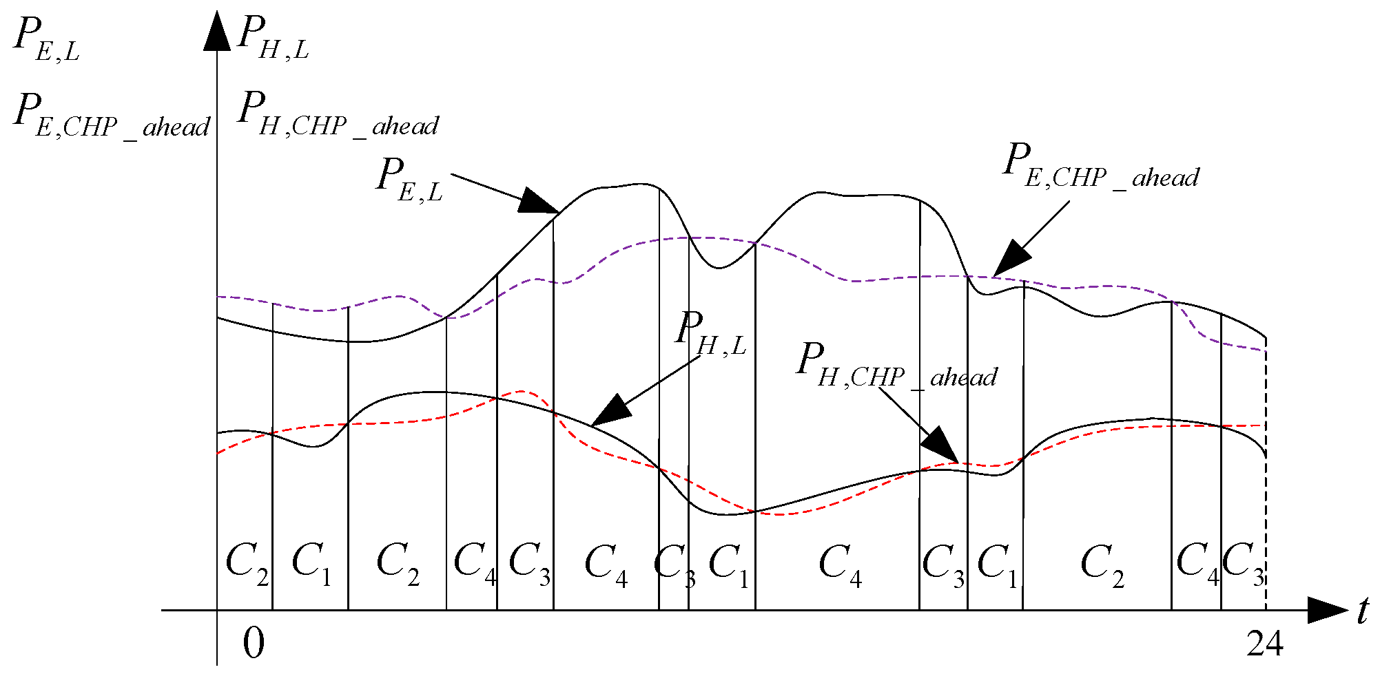
In this paper, the nominal capacity of the adopted network-connected CHP is 1 MW. Other parameters are shown in Table A2 in the Appendix. In Figure 8, the heat and electric demand are from historical data of a new residential district in Braunschweig Germany, which was measured and recorded at intervals of fifteen minutes during one year [30,31]. P_E,CHP and P_H,CHP are the electric and heat output of CHP, respectively, which are obtained from the day-ahead operating data. It is easily found that the sum of P_E,CHP and P_H,CHP is the nominal capacity of the CHP, 1 MW. The heat load is high at night, about 0.7 MW, and low in the daytime, reaching a minimum value 0.35 MW at about 14:30. On the contrary, the electric load is low at night, the minimum being 0.3 MW at 24:00, and rather high in the daytime, reaching a maximum 1 MW at 11:00. Around 12:00, the electric load drops a little for the short break at noon. The load condition determines the operation modes of the CHP. During the night, the output of CHP is mainly in the form of heat to satisfy heat demand and the HTER is at a high value. In the daytime, the CHP is operated at a low HTER level to produce more electricity to satisfy the electric demand.

The prices of natural gas, buying and selling heat and electricity are shown in Figure 9 [32]. From Figure 9a,b, we can find that the prices of selling heat and electricity to the networks are lower than those of buying them. The highest electricity buying and selling price are at around 10:00, about 0.519 Euro/kWh and 0.3 Euro/kWh, respectively. The lowest prices happen at 24:00, just about 0.003 Euro/kWh and 0.001 Euro/kWh, respectively. While the highest heat buying price (0.045 Euro/MJ) and selling price (0.02 Euro/MJ) occurs at 1:00 and 10:30, respectively. The lowest two prices for heat are 0.009 Euro/kWh and 0.003 Euro/MJ at 14:00 and 7:30, respectively. Compared to the heat and electricity price, the price of the natural gas fluctuates at a smaller range.

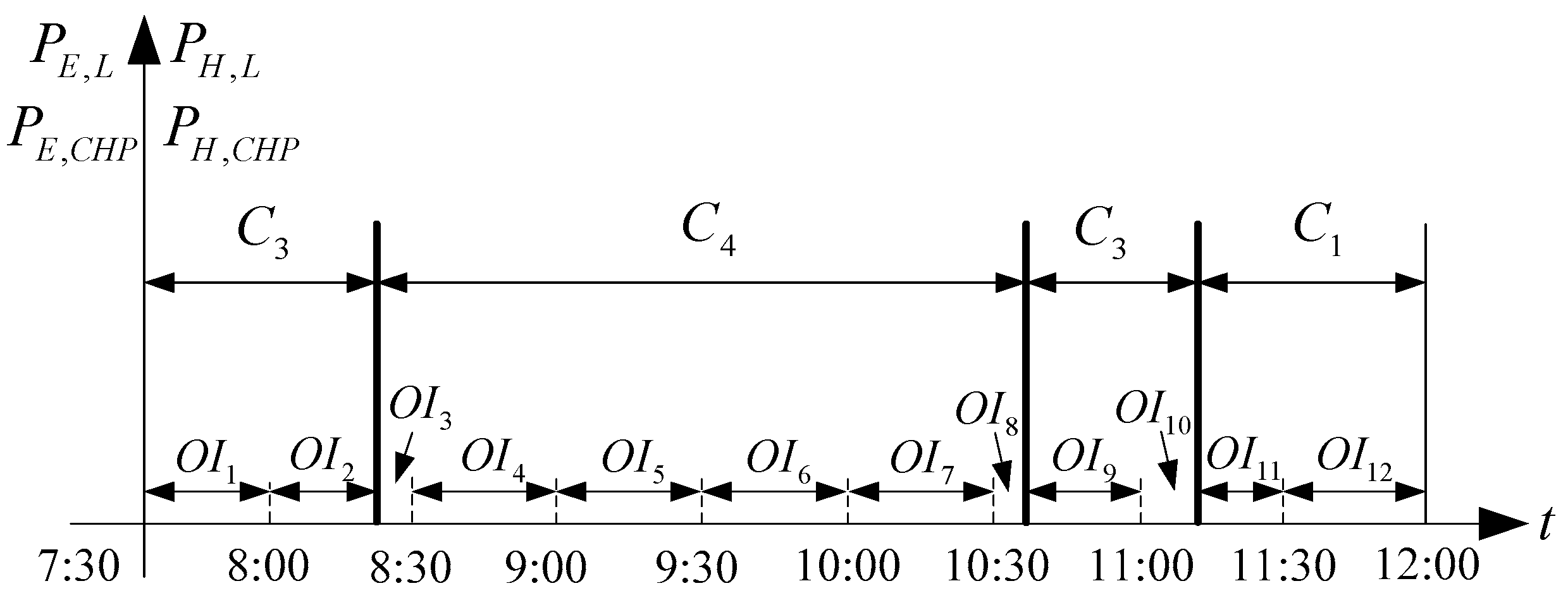
Based on Figure 8 and Figure 9, the operation modes of the CHP can be identified, shown in

Table 1. Operation modes of CHP in real time.

Time	Modes	Time	Modes	Time	Modes	Time	Modes
0:00–0:30	C3	6:00–6:30	C2	13:00–13:30	C3	19:00–19:30	C2
0:30–1:00	C3	6:30–7:00	C2	13:30–14:00	C3	19:30–19:50	C2
1:00–1:15	C3	7:00–7:10	C2	14:00–14:30	C3	19:50–20:00	C4
1:15–1:30	C2	7:10–7:30	C4	14:30–15:00	C3	20:00–20:30	C4
1:30–2:00	C2	7:30–8:00	C4	15:00–15:30	C3	20:30–20:45	C4
2:00–2:30	C2	8:00–8:30	C4	15:30–16:00	C3	20:45–21:00	C3
2:30–3:00	C2	8:30–9:00	C4	16:00–16:30	C3	21:00–21:30	C3
3:00–3:30	C2	9:00–9:30	C4	16:30–16:45	C3	21:30–21:50	C3
3:30–3:40	C2	9:30–10:00	C4	16:45–17:00	C2	21:50–22:00	C1
3:40–4:00	C3	10:00–10:30	C4	17:00–17:30	C2	22:00–22:15	C1
4:00–4:30	C3	10:30–11:00	C4	17:30–17:50	C2	22:15–22:30	C2
4:30–5:00	C3	11:00–11:30	C4	17:50–18:00	C4	22:30–22:45	C2
5:00–5:30	C3	11:30–12:00	C3	18:00–18:20	C4	22:45–23:00	C3
5:30–5:50	C3	12:00–12:30	C3	18:20–18:30	C2	23:00–23:30	C3
5:50–6:00	C2	12:30–13:00	C3	18:30–19:00	C2	23:30–24:00	C1

. All four modes occur in one day, and C₃ appears with the maximum number. In Mode C₃, the electric demand is high, and the deficit is satisfied by buying additional electricity from the network. Modes C₂ and C₄ also exist, where additional heat or both additional heat and electricity are bought from the corresponding networks. However, Mode C₁ only exists between 21:50 and 22:15, 23:30 and 24:00. Only at night, when the heat and electric demand happen to be both at a low level, are the extra heat and electricity sold to the networks. In the other modes, the CHP is modified to a certain level of HTER to satisfy at least one kind of load as much as possible.

Based on the 60 OIs in Table 1, the profits of the CHP at different operation points in real time are obtained, shown in Figure 10.

In Figure 10, the colorful figure is the profit distribution for CHP at different loading levels. The black line is the optimal operation points for CHP where the profits are maximized, and the value is shown in

Table 2. Maximum profit of the CHP in real time.

Time	Profit (Euro)	Time	Profit (Euro)	Time	Profit (Euro)	Time	Profit (Euro)
0:00–0:30	2.04	6:00–6:30	4	13:00–13:30	−149.2	19:00–19:30	7.55
0:30–1:00	2.19	6:30–7:00	4.48	13:30–14:00	−119.9	19:30–19:50	12.07
1:00–1:15	0.83	7:00–7:10	4.3	14:00–14:30	−110.2	19:50–20:00	0.78
1:15–1:30	0.01	7:10–7:30	−11.2	14:30–15:00	−80.78	20:00–20:30	−9.95
1:30–2:00	0.4	7:30–8:00	−28	15:00–15:30	−50.6	20:30–20:45	−0.92
2:00–2:30	−0.77	8:00–8:30	−43.46	15:30–16:00	−27.61	20:45–21:00	−7.14
2:30–3:00	0.86	8:30–9:00	−58.01	16:00–16:30	−21.15	21:00–21:30	−14.13
3:00–3:30	0.56	9:00–9:30	−73.26	16:30–16:45	−1.71	21:30–21:50	−0.85
3:30–3:40	0.29	9:30–10:00	−95.82	16:45–17:00	1.91	21:50–22:00	1.75
3:40–4:00	0.15	10:00–10:30	−119.3	17:00–17:30	2.63	22:00–22:15	2.01
4:00–4:30	−0.56	10:30–11:00	−99.92	17:30–17:50	1.63	22:15–22:30	0.54
4:30–5:00	−0.67	11:00–11:30	−79.91	17:50–18:00	1.69	22:30–22:45	0.12
5:00–5:30	−1.51	11:30–12:00	−76.96	18:00–18:20	0.59	22:45–23:00	0.52
5:30–5:50	−2.51	12:00–12:30	−72.01	18:20–18:30	2.06	23:00–23:30	1.61
5:50–6:00	1.22	12:30–13:00	−153.8	18:30–19:00	8.91	23:30–24:00	0.65

. The positive value in Table 2 means extra profit is obtained, and the negative value means the energy purchasing fee has to be paid, which has been minimized. From Figure 10, the maximum profits occur between 0:00 and 7:00, 15:00 and 24:00, where the profits are mostly positive. The profit reaches its maximum (12.07 Euro) between 19:30 and 19:50. Between 7:10 and 16:45, the profits for CHP are all negative. The phenomenon is caused by the high electric demand. The electric load cannot be satisfied at noon, although the electricity output of CHP reaches its maximum. Thus, a lot of electricity has to be bought from the electric network at a high price. The maximum energy purchasing fee is about 150 Euro between 12:30 and 13:00. Of course, the fee has been minimized through modifying the output of the CHP. It can be found that the profit of CHP is determined a lot by the electricity price for its value is higher than that of the heat. Through optimization, the community’s expense to buy energy is reduced to the minimum, and net profit reaches the maximum in real time.

Before optimization, the profit of the CHP is shown in

Table 3. Profit of the CHP using the day-ahead operation curve before optimizing.

Time	Profit (Euro)	Time	Profit (Euro)	Time	Profit (Euro)	Time	Profit (Euro)
0:00–0:30	1.97	6:00–6:30	3.98	13:00–13:30	−157.00	19:00–19:30	7.54
0:30–1:00	2.10	6:30–7:00	4.48	13:30–14:00	−123.67	19:30–19:50	12.02
1:00–1:15	0.81	7:00–7:10	4.28	14:00–14:30	−113.83	19:50–20:00	−1.42
1:15–1:30	−0.03	7:10–7:30	−11.82	14:30–15:00	−83.68	20:00–20:30	−18.40
1:30–2:00	0.34	7:30–8:00	−29.11	15:00–15:30	−52.71	20:30–20:45	−2.15
2:00–2:30	−0.81	8:00–8:30	−55.05	15:30–16:00	−28.64	20:45–21:00	−7.52
2:30–3:00	0.81	8:30–9:00	−71.85	16:00–16:30	−21.99	21:00–21:30	−14.33
3:00–3:30	0.50	9:00–9:30	−97.61	16:30–16:45	−1.78	21:30–21:50	−0.96
3:30–3:40	0.27	9:30–10:00	−124.17	16:45–17:00	1.88	21:50–22:00	1.75
3:40–4:00	0.08	10:00–10:30	−147.73	17:00–17:30	2.57	22:00–22:15	2.01
4:00–4:30	−0.68	10:30–11:00	−121.56	17:30–17:50	1.59	22:15–22:30	0.51
4:30–5:00	−0.69	11:00–11:30	−96.42	17:50–18:00	1.65	22:30–22:45	0.10
5:00–5:30	−1.66	11:30–12:00	−79.65	18:00–18:20	0.45	22:45–23:00	0.51
5:30–5:50	−2.68	12:00–12:30	−74.90	18:20–18:30	2.04	23:00–23:30	1.61
5:50–6:00	1.20	12:30–13:00	−159.90	18:30–19:00	8.90	23:30–24:00	0.66

. The community’s total profit for a day is −1,637.82 Euro. By comparison, the optimized total profit from Table 2 is −1,443.46 Euro, reducing community’s energy cost by about 11.87%.

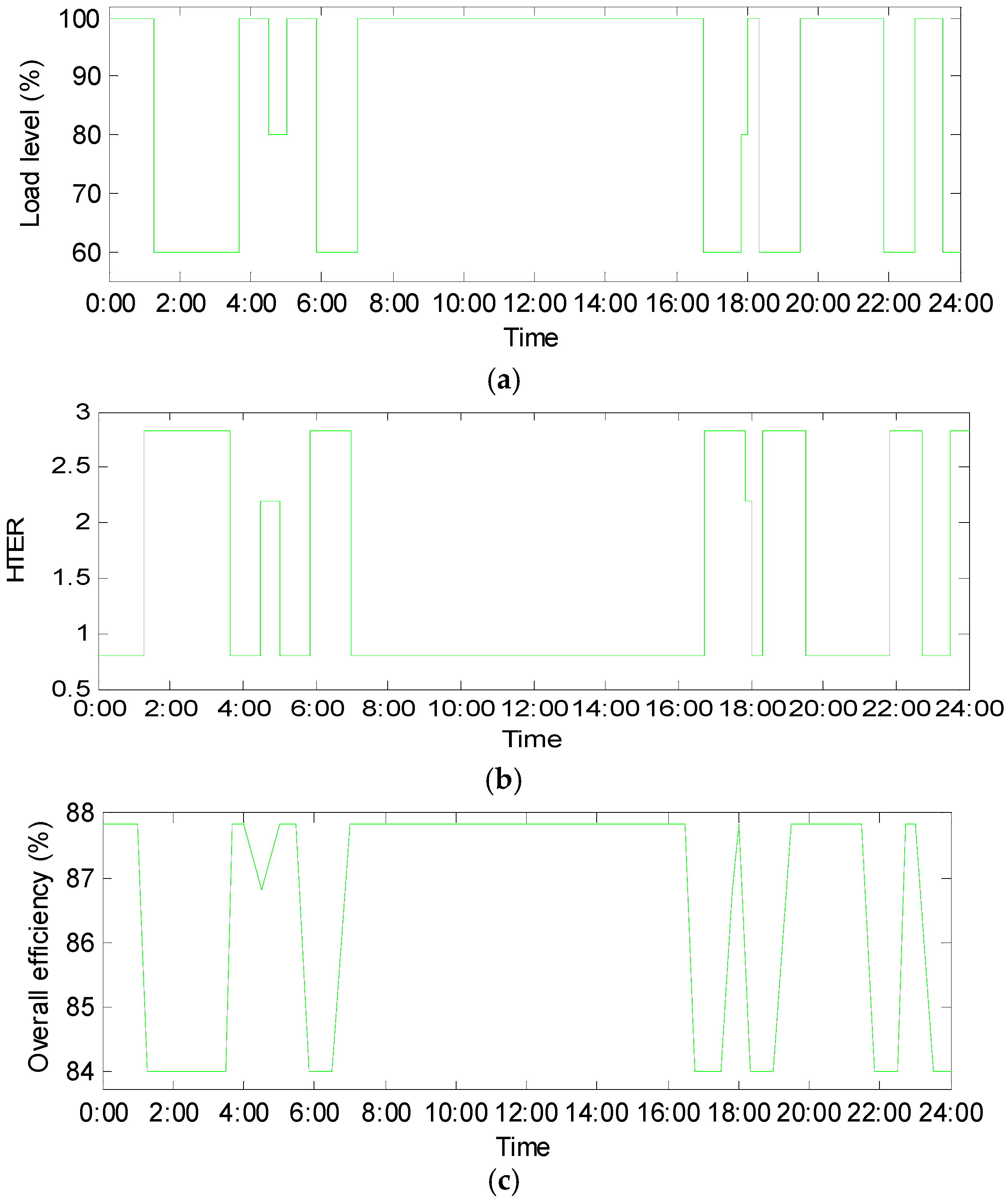
The loading level, HTER and overall efficiency for the optimal operation points in Figure 10 are shown in Figure 11. The optimal loading level varies a lot in the night time, mostly at 60%, and the corresponding HTER is at a high value of 2.83, with the optimal efficiency around just 84%. In the daytime, the CHP is at full load, with a low HTER and high efficiency, 0.8% and 87.8%, respectively.

It is also found that high loading level does not always mean high profit for the residents. The HTER also affects the profit a lot. Comparing Figure 11a to Figure 11b, when the loading level is high, the HTER is at a low value to produce more electricity. Correspondingly, when the loading level is low, the HTER is at a high value to produce more heat to satisfy the heat load first. The HTER and efficiency are both functions of the loading level.

5. Conclusions

In this paper, the model of network-connected CHP was established. Then, based on the relationship between heat and electric output, the profit model for the CHP is derived by using a discrete optimization model. The conclusions are drawn as follows:

•

There mainly exist four operation modes for network-connected CHP, determined by the relationship between the energy demand and supply. Based on the OI determined by operation modes and real-time prices, the operation of CHP can be optimized in a discrete way.

•

The profit is determined by electric prices because it is usually high or much higher than that of heat. Thus, in the daytime, the CHP is operated at a high loading level to gain a low value of HTER to produce more electricity. At night, the CHP is operated at a low loading level to gain a higher value of HTER for more heat production.

•

A high loading level or high output does not always mean high profits. The loading level affects the HTER and overall efficiency of CHP tremendously. Under different load conditions and energy price scenarios, the CHP should use different optimal operation strategies.