Article

A New Predictive Model Based on the ABC Optimized Multivariate Adaptive Regression Splines Approach for Predicting the Remaining Useful Life in Aircraft Engines

1
Department of Mathematics, Faculty of Sciences, University of Oviedo, C/Calvo Sotelo s/n, 33007 Oviedo, Spain
2
Department of Mining Technology, Topography and Structures, University of León, 24071 León, Spain
*
Author to whom correspondence should be addressed.
Energies 2016, 9(6), 409; https://doi.org/10.3390/en9060409
Submission received: 7 March 2016 / Revised: 19 May 2016 / Accepted: 23 May 2016 / Published: 26 May 2016

Abstract

:
Remaining useful life (RUL) estimation is considered as one of the most central points in the prognostics and health management (PHM). The present paper describes a nonlinear hybrid ABC–MARS-based model for the prediction of the remaining useful life of aircraft engines. Indeed, it is well-known that an accurate RUL estimation allows failure prevention in a more controllable way so that the effective maintenance can be carried out in appropriate time to correct impending faults. The proposed hybrid model combines multivariate adaptive regression splines (MARS), which have been successfully adopted for regression problems, with the artificial bee colony (ABC) technique. This optimization technique involves parameter setting in the MARS training procedure, which significantly influences the regression accuracy. However, its use in reliability applications has not yet been widely explored. Bearing this in mind, remaining useful life values have been predicted here by using the hybrid ABC–MARS-based model from the remaining measured parameters (input variables) for aircraft engines with success. A correlation coefficient equal to 0.92 was obtained when this hybrid ABC–MARS-based model was applied to experimental data. The agreement of this model with experimental data confirmed its good performance. The main advantage of this predictive model is that it does not require information about the previous operation states of the aircraft engine.

1. Introduction

An aircraft engine is the component of the propulsion system for an aircraft that generates mechanical power. Aircraft engines are almost always either lightweight piston engines or gas turbines [1,2]. A gas turbine, also called a combustion turbine, is a type of internal combustion engine. It has an upstream rotating compressor coupled to a downstream turbine, and a combustion chamber in between. The basic operation of the gas turbine is similar to that of the steam power plant except that air is used instead of water. Fresh atmospheric air flows through a compressor that brings it to higher pressure. Energy is then added by spraying fuel into the air and igniting it so the combustion generates a high-temperature flow. This high-temperature high-pressure gas enters a turbine, where it expands down to the exhaust pressure, producing a shaft work output in the process. The turbine shaft work is used to drive the compressor and other devices such as an electric generator that may be coupled to the shaft [3,4]. The energy that is not used for shaft work comes out in the exhaust gases, so these have either a high temperature or a high velocity. The purpose of the gas turbine determines the design so that the most desirable energy form is maximized. Gas turbines are used to aircraft engines, trains, ships, electrical generators, and even tanks [3,4,5,6]. Indeed, the engine diagram in Figure 1 shows the main elements of the engine model. Additionally, Figure 2 shows the flowchart corresponding to the simulation with its modules.
A particularly important concept is the prognostics of the aircraft turbine engine components. Indeed, prognostics is defined as an engineering discipline focused on predicting the time at which a system or a component will no longer perform its intended function. This lack of performance is most often a failure beyond which the system can no longer be used to meet desired performance [7]. Prognostics is a very important aspect of an equipment health management system. A reliable prognostic system provides some benefits in terms of the financial cost saving and safety. The prerequisite of the benefit from the prognostics is the correct detection of fault by an efficient diagnostic system because diagnostic decision triggers the prognostic system [8]. The predicted time then becomes the remaining useful life (RUL) [9,10,11,12,13], which is an important concept in decision making for contingency mitigation. Therefore, prognostics is explicitly defined as the estimation of the remaining useful life (RUL) of any equipment. The science of prognostics is based on the analysis of failure modes, detection of early signs of wear and aging, and fault conditions.
It is to be noted that the safe and reliable operation of engineering systems such as aircraft engines is of great significance for modern energy plants, production quality, preservation of human health and life, etc. [14,15]. In this way, reliability is theoretically defined as the probability of failure, the frequency of failures, or in terms of availability, a probability derived from reliability and maintainability. Specifically, the concept of remaining useful life (RUL) is defined here as the number of remaining time units that the equipment has before it reaches the limit for a safe operation [7,8,9,10,11,12,13,14,15,16].
Taking into account that the RUL of any device can be considered as a random variable [17], since it depends on some variables that are properties of each equipment such as its age, the operation environment and the operation conditions, a statistical approach of this operation variable would be a convenient method. Previous studies have tried to predict the RUL based on time series [18,19]. However, nowadays it is more useful to use models based on the monitoring of the operation variables values during the operation of the equipment [20,21]. Therefore, the present study uses this approach.
The objective of this study is to evaluate the application of the multivariate adaptive regression splines (MARS) approach in combination with the Artificial Bee Colony (ABC) technique for the calculation of a predictive model of the RUL for aircraft engines. The MARS technique is based on the statistical learning theory and is a new class of models that can be used to predict values in very different areas [22,23,24,25,26]. This study uses multivariate adaptive regression splines (MARS), a nonlinear and non-parametric regression methodology, to build a RUL forecasting model from experimental turbines data. It is a nonparametric regression technique and can be seen as an extension of linear models that automatically model nonlinearities and complex interactions between variables. The statistical learning theory is the theoretical foundation for the learning algorithm of the MARS technique [22,23,24,25,26,27]. Some motivations behind the application of the proposed method with respect to other already existing techniques are as follows: (1) MARS models are more flexible than linear regression models; (2) MARS models are simple to understand and interpret; (3) MARS can handle both continuous and categorical data; (4) MARS models tend to have a good bias-variance trade-off; and (5) MARS models give us an explicit mathematical formula of the dependent variable as a function of the independent variables through an expansion of basis functions (hinge functions and products of two or more hinge functions). This last feature is a fundamental difference compared to other alternative methods because most of them behave like a black box. In order to carry out the optimization mechanism corresponding to the optimal hyperparameters setting in the MARS training, the artificial bee colony (ABC) technique was used here with success. The artificial bee colony (ABC) technique is an optimization algorithm based on the intelligent foraging behavior of honeybee swarms [28]. Similar to other evolutionary computation algorithms such as particle swarm optimization (PSO) [29,30,31] or ant colony optimization [32], ABC exploits the model of social sharing of information [28,33,34]. For the above-mentioned purpose, a hybrid ABC optimized MARS (ABC–MARS) model was used as an automated learning tool, training it in order to predict remaining useful life (RUL) from other turbine’s operation parameters. According to previous research, the MARS technique has been proven to be an effective tool to predict natural parameters, being successfully used in a wide range of environmental fields: medical applications [35,36], forest modeling [37], prediction of the air quality [38], water quality studies [39,40], solution of geotechnical problems, particularly those that lack a precise analytical theory or understanding of the phenomena involved [41], and so on.
In summary, the present study is structured as follows: firstly, the materials, methods and dataset used are explained; secondly, the results of the new hybrid ABC–MARS-based model trained are presented and discussed; and finally, the main conclusions of this research work are drawn. Therefore, the aim of this research work was to obtain a predictive model for the RUL as well as the contribution degree of each input operation parameter.

2. Materials and Methods

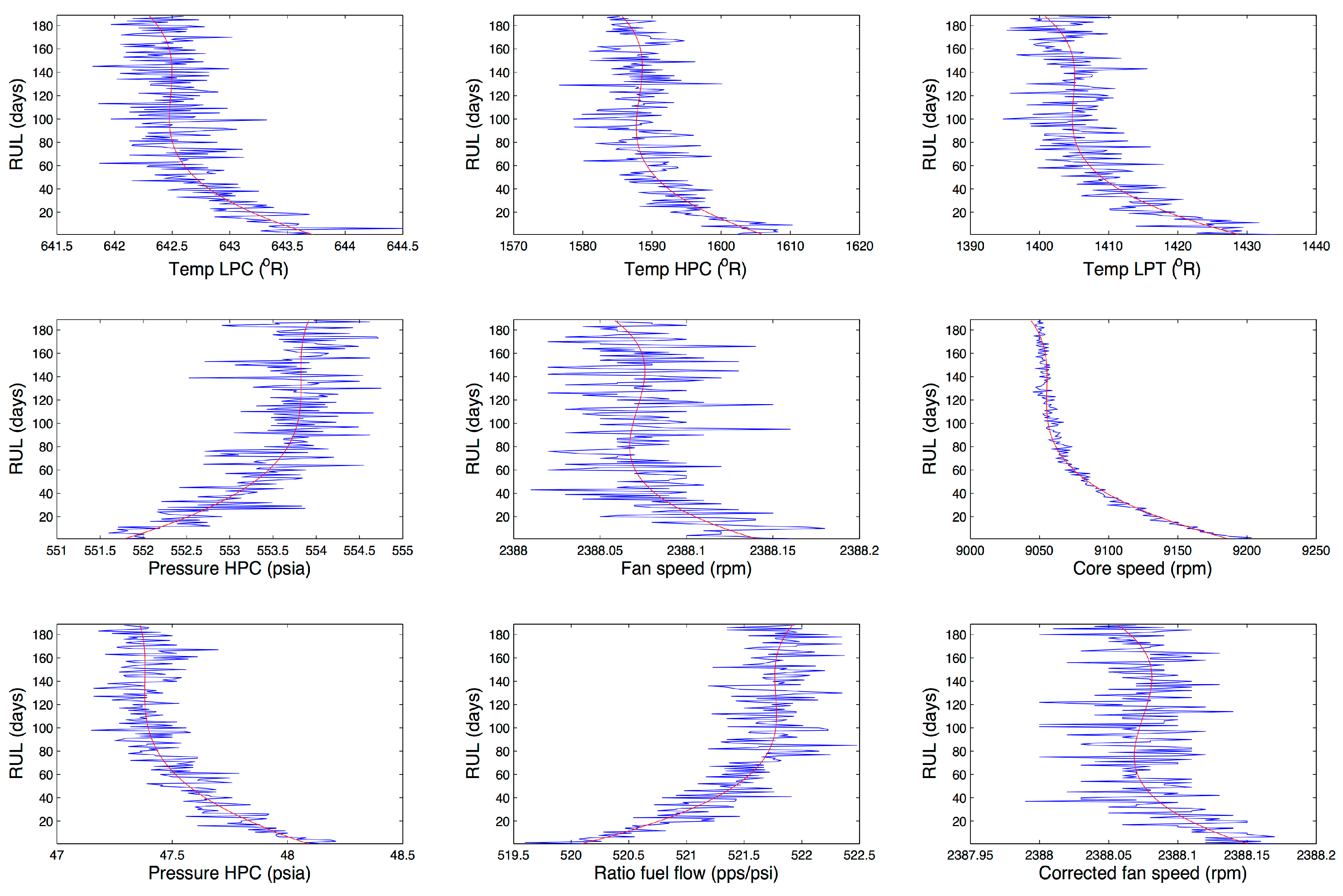
2.1. Experimental Dataset

The present study uses a dataset corresponding to an aircraft engine of 90,000 lbs. thrust class. Indeed, this dataset includes working conditions with heights from sea conditions to 40,000 feet and temperatures from −51 °C to 39 °C. Specifically, the above dataset was obtained through a software application known as MAPSS (Modular Aero-Propulsion System Simulation) [42]. This is a simulation environment for aeronautical turbines that allows access to a range of monitoring parameters controlling the operating state of the system through a graphical user interface. This provides the user with a simulation environment that is able to develop advanced algorithms for control and diagnosis that can be tested on a generic aircraft engine simulator. Additionally, MAPSS is able to generate linear state space models from which the user can create linear controls. Furthermore, MAPSS is also able to perform simulations of transient states. These capabilities allow the user to verify the performance of the control algorithms and its validation in a generic engine model [42]. The MAPSS program has two well-known versions for both civil and military applications. As a final note, the military version is able to perform realistic simulations within the FADEC (Full Authority Digital Engine Controllers) [43] standard and it will be used for the present research.
The database of the study consists of data for a total of 100 turbines, with a number of observations that ranges from 128 to 362 for each one, being the dependent variable in the RUL. The total number of observations for all of the turbines amounts to 20,631 observations. The database contains input parameters that simulate the effects of faults and deterioration in any of the rotating components of the engine (fan, LPC, HPC, HPT, and LPT). Data belong to a fleet of similar aircrafts with the same engines. It is important to emphasize that each engine starts with a different health status but at the beginning all are inside the operational range and the dataset convers since that moment to the engine failure.
Note that each record of the engine state is formed by a set of 24 variables, three of them are operational settings and the other 21 represent values for engine performance measurements, which are contaminated with noise. A complete list of variables is presented in Table 1. The operability margins, such as stall and temperature margins, define the safe operation region for the engine [44]. Six different flight conditions are contained in the database, with altitudes from 0 to 42,000 feet, speeds from 0 to 0.84 Mach and throttle resolver angle from 20° to 100°. For further information about how the engine run-to-failure simulation is performed, the readers can consult the reference [42].
After a first exploratory analysis, it was found that the measurements of the variables Total temperature at fan inlet, Pressure at fan inlet, Engine pressure ratio, Burner fuel-air ratio, Demanded fan speed and Demanded corrected fan speed are constant and that variable Total pressure in bypass-duct oscillates between 21.6 and 21.61 psia. Therefore, these variables will not be used in the calculations. Additionally, the absolute value of the correlation coefficients between each pair of variables is graphically represented by the correlation matrix [25,26] in Figure 3. Two additional variables, Physical core speed (C_sp) and Corrected core speed (C_csp), were discarded due to their low correlation with the independent variable RUL. Indeed, only the remaining twelve variables are used as independent variables in the modeling of the dependent variable RUL and its simulation. As an example, Figure 4 shows the 189 observations of the independent and dependent variables for the turbine 4.
The RUL prognosis is a complex and highly nonlinear problem. Figure 4 shows that RUL is a multivariate function of the operating parameters of the turbofan engines. In general, there are two major approaches to prognostics: physics-based and data-driven models. In the first case one needs to build an accurate physical model of system behavior either in normal state or in faulty conditions. Comparing the data captured from the sensors to the model predictions, one can obtain the health indicator of the system. In the second case, there is no physical model but the data with relevant events are available. On the one hand, physics-based models require the presence of a mathematical representation of the physics of failure degradation and the parameters used in degradation modeling. On the other hand, data-driven models require statistically sufficient run-to-failure samples, due to the fact that RUL of turbofan engine can be considered as a random variable [17], since it depends on the properties of the equipment such as its age, the operation environment and the operation conditions.
The dataset that has been analyzed is adequate for data-driven approach since sufficient data and RUL values are available with dataset. The ABC–MARS-based model is suitable for this case in order to achieve an effective approach to nonlinearities present in this regression problem. Additionally, it is not appropriate for physics-based modeling since the health index parameters are not given, and no physics-based model found for whole engine system degradation. Accordingly, the database referred previously will be used for the training and validation of the hybrid model proposed in this paper using a random 90% of the information for training and the remaining 10% for validation.

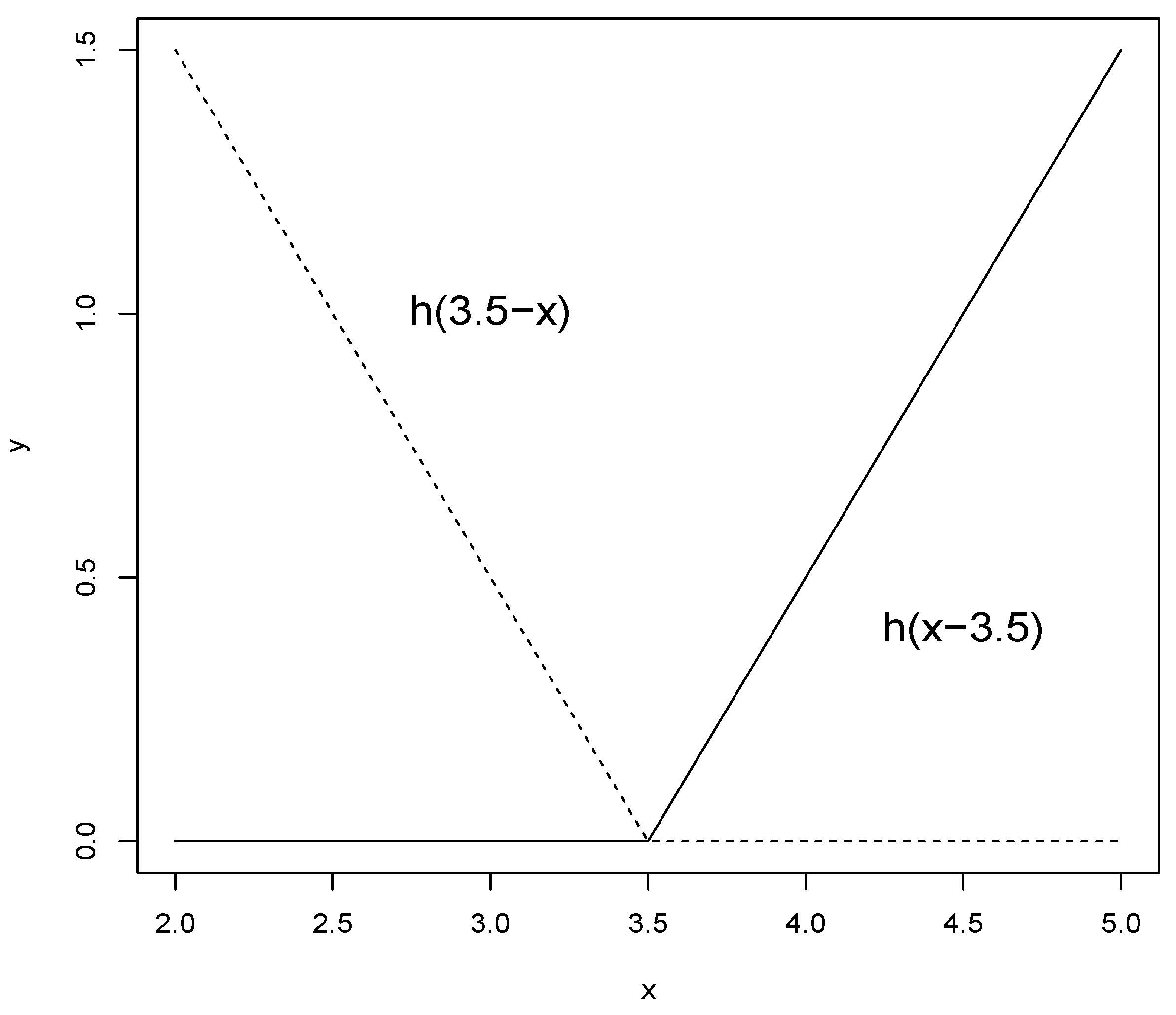
2.2. Multivariate Adaptive Regression Splines (MARS)

Multivariate adaptive regression splines (MARS) is a multivariate nonparametric classification/regression technique [22,23,24]. Its main purpose is to predict the values of a continuous dependent variable, y ( n × 1 ) , from a set of independent explanatory variables, X ( n × p ) . The MARS model can be represented as:
y = f ( X ) + e
where f is a weighted sum of basis functions that depend on X and e is an error vector of dimension ( n × 1 ) .
MARS model does not require any a priori assumptions about the underlying functional relationship between dependent and independent variables. Instead, this relation is uncovered from a set of coefficients and piecewise polynomials of degree q (basis functions) that are entirely “driven” from the regression data ( X , y ) . The MARS regression model is constructed by fitting basis functions to distinct intervals of the independent variables. Generally, piecewise polynomials, also called splines, have pieces smoothly connected together. In MARS terminology, the joining points of the polynomials are called knots, nodes or breakdown points. These will be denoted by the small letter t. For a spline of degree q each segment is a polynomial function. MARS uses two-sided truncated power functions as spline basis functions, described by the following equations [22,23,24,27,35,36,37,38,39,40]:
[ ( x t ) ] + q = { ( t x ) q i f    x < t 0 o t h e r w i s e
[ + ( x t ) ] + q = { ( t x ) q i f    x t 0 o t h e r w i s e
where q ( 0 ) is the power to which the splines are raised and which determines the degree of smoothness of the resultant function estimate. When q = 1 , which is the case in this study, only simple linear splines are considered. A pair of splines for q = 1 at the knot t = 3.5 is presented in Figure 5.
The MARS model of a dependent variable y with M basis functions (terms) can be written as [22,23,24,27,35,36,37,38,39,40]:
y ^ = f ^ M ( x ) = c 0 + m = 1 M c m B m ( x )
where y ^ is the dependent variable predicted by the MARS model, c0 is a constant, B m ( x ) is the m-th basis function, which may be a single spline basis functions, and c m is the coefficient of the m-th basis functions.
Both the variables to be introduced into the model and the knot positions for each individual variable have to be optimized. For a dataset X containing n objects and p explanatory variables, there are N = n × p pairs of spline basis functions, given by Equations (2) and (3), with knot locations x i j ( i = 1 , 2 , , n ;    j = 1 , 2 , , p ).
A two-step procedure is followed to construct the final model. First, in order to select the consecutive pairs of basis functions of the model, a two-at-a-time forward stepwise procedure is implemented [22,23,24,27,35,36,37,38,39,40]. This forward stepwise selection of basis function leads to a very complex and overfitted model. Such a model, although it fits the data well, has poor predictive abilities for new objects. To improve the prediction, the redundant basis functions are removed one at a time using a backward stepwise procedure. To determine which basis functions should be included in the model, MARS utilizes the generalized cross-validation (GCV) [27,35,36,37,38,39,40]. In this way, the GCV is the mean squared residual error divided by a penalty dependent on the model complexity. The GCV criterion is defined in the following way [22,23,24,27,35,36,37,38,39,40]:
G C V ( M ) = 1 n i = 1 n ( y i f ^ M ( x i ) ) 2 ( 1 C ( M ) / n ) 2
where C ( M ) is a complexity penalty that increases with the number of basis functions in the model and is defined as [22,23,24,27,35,36,37,38,39,40]:
C ( M ) = ( M + 1 ) + d M
where M is the number of basis functions in Equation (4), and the parameter d is a penalty for each basis function included into the model. It can be also regarded as a smoothing parameter. Large values of d lead to fewer basis functions and therefore smoother function estimates.
Once the MARS model is constructed, it is possible to evaluate the importance of the explanatory variables used to construct the basis functions. Establishing predictor importance is in general a complex problem, which in general requires the use of more than one criterion. In order to obtain reliable results, it is convenient the use of the GCV parameter explained before together with the parameters Nsubsets (criterion counts the number of model subsets in which each variable is included) and the residual sum of squares RSS [22,23,24,27,35,36,37,38,39,40].

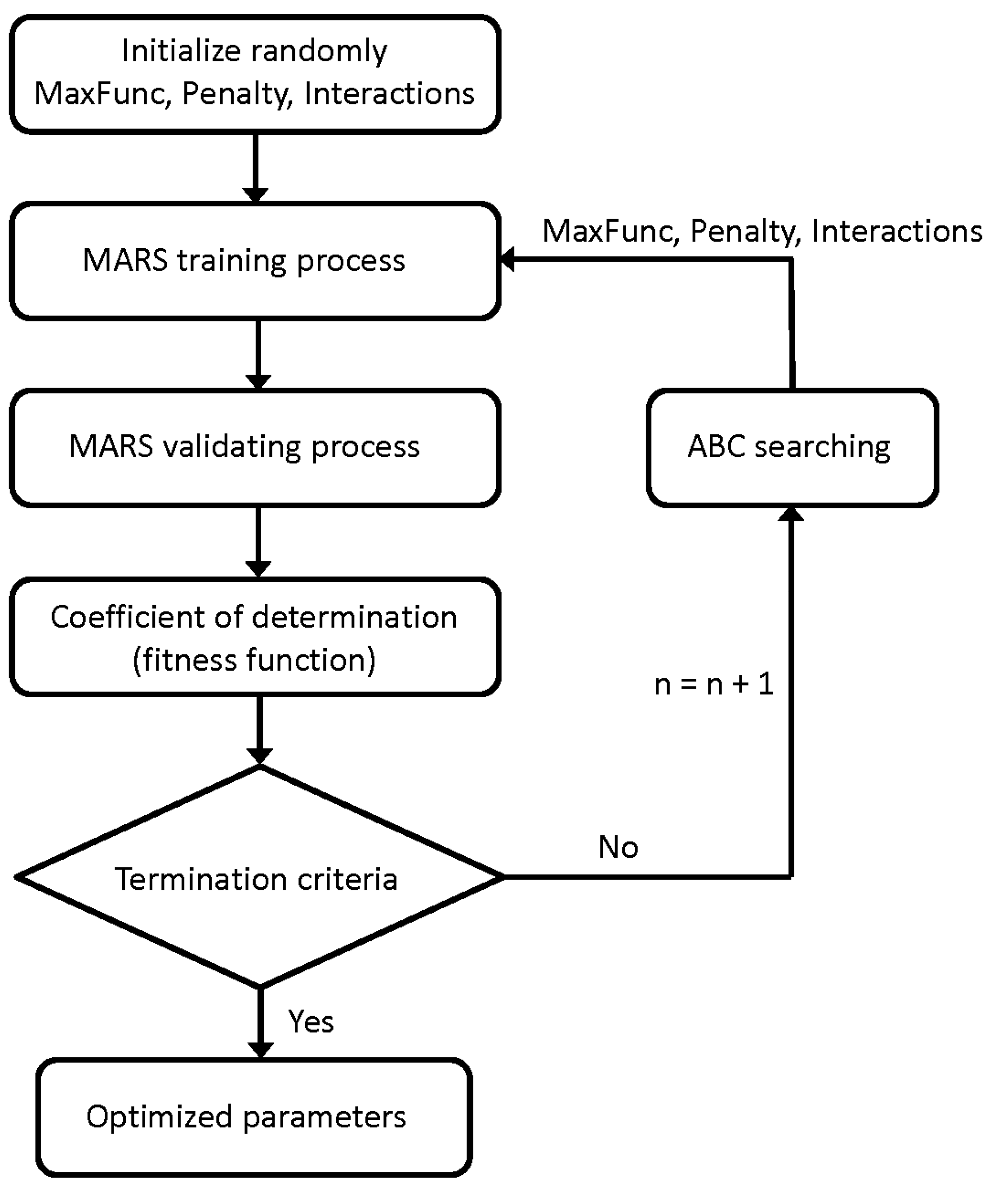
2.3. The Artificial Bee Colony (ABC) Algorithm

The algorithm Artificial Bee Colony (ABC) is an evolutionary optimization algorithm inspired in the behavior of bees foraging food sources [28,33,34]. Indeed, in the ABC technique, the colony consists of three groups of bees: employed bees, onlookers and scouts. The N food sources are the possible set of solutions and are represented by the vectors p i . It represents its position in the search space of possible solutions. The food source dimension is the number of parameters of the optimization problem. The algorithm initializes the food sources or possible solutions of the problem randomly in a plausible hypercube and the fitness of each food source is evaluated. The relation between the objective function F and the fitness of a food source is given by (see Figure 6):
F i t n e s s ( F ( p i ) ) = { 1 1 + F ( p i ) if F ( p i ) > 0 1 + | F ( p i ) | if F ( p i ) 0     i = 1 , , N
The lower the objective function value, the higher the fitness. As the algorithm searches for the highest fitness of a food source, it minimizes. The ABC technique has three phases [28,33,34]:
  • The Employee Bee Phase
In the first phase, the employee bees forage the food sources and tries to introduce a variation of every i food source according with the equation [28,33,34]:
v i j = p i j + R i j ( p k j p i j )
where j is the randomly chosen parameter we are modifying, k a randomly chosen food source different from i and R i j a number chosen randomly in [−1,1]. Once v i j is calculated, its fitness is obtained. If this is higher than f i t n e s s ( F ( p i j ) ) , its value is changed to v i j and the trial counter set to one. If not, the value of the food source does not change and the trial counter is increased.
  • The Onlooker Bee Phase
For each food source p i , we draw a number r i in [ 0 , 1 ] . If r i < p r o b i , we try again to change one parameter in the food source. The quantity p r o b i is obtained from the fitness of this food source as follows [28,33,34]:
p r o b i = 0.9 F i t n e s s ( F ( p i ) ) max k = 1 , , N ( F i t n e s s ( F ( p k ) ) ) + 0.1
  • The Scout Bee Phase
If, after a determined number of trials, a food source is not improved, it is discarded and a new one is randomly chosen from the initial searching space. The food source with the highest fitness is the temporal optimum in this iteration [28,33,34]. This cycle is continued until a stop condition is met. In the present case, the stop condition has been a maximum number of iterations and the repetition of the optimum for a determined number of iterations. If this occurs, it is assumed that the algorithm has already converged.

2.4. Algorithm Goodness-of-Fit Measurement

To estimate remaining useful life from other parameters measured in the aircraft engines, it is important to select the model that best fits the experimental data. The criterion considered in this research to measure the goodness-of-fit was the coefficient of determination R2 [45,46,47]. This ratio indicates the proportion of total variation in the dependent variable explained by the model (inside-bark volume in our case). A dataset takes values ti, each of which has an associated modeled value y i . The former are called the observed values and the latter are often referred to as the predicted values. Variability in the dataset is measured through different sums of squares [45,46,47]:
  • S S t o t = i = 1 n ( t i t ¯ ) 2 : The total sum of squares, proportional to the sample variance.
  • S S r e g = i = 1 n ( y i t ¯ ) 2 : The regression sum of squares, also called the explained sum of squares.
  • S S e r r = i = 1 n ( t i y i ) 2 : The residual sum of squares.
In the previous sums, t ¯ is the mean of the n observed data:
t ¯ = 1 n i = 1 n t i
Bearing in mind the above sums, the general definition of the coefficient of determination is:
R 2 1 S S e r r S S t o t
A coefficient of determination value of 1.0 indicates that the regression curve fits the data perfectly.

3. Analysis of Results and Discussion

The total number of predicting variables used to build the hybrid ABC–MARS model was 12. The output predicted variable was the remaining useful life.
Furthermore, it is well known that the MARS technique is strongly dependent on the following hyperparameters [22,23,24,27,35,36,37,38,39,40]:
  • Maximum number of basis functions (Maxfuncs): Maximum number of model terms before pruning, i.e., the maximum number of terms created by the forward pass.
  • Penalty parameter (d): The Generalized Cross Validation (GCV) penalty per knot. A value of 0 penalizes only terms, not knots. The value −1 means no penalty.
  • Interactions: Maximum degree of interaction between variables.
Some methods often used to determine suitable hyperparameters are [22,23,24,27,35,36,37,38,39,40]: grid search, random search, Nelder–Mead search, heuristic search, genetic algorithms, pattern search, etc. In this research work, the Artificial Bee Colony (ABC) technique was applied [28,33,34].
Therefore, a hybrid ABC–MARS-based model was applied to predict the RUL (output variable) from the other twelve remaining variables (input variables) studying their influence in order to optimize its calculation through the analysis of the determination coefficient R2 with success. Figure 7 shows the flowchart of this hybrid ABC–MARS-based model developed in this research work.
The determination coefficient is a statistical measure of how well a regression curve approximates real data points. Furthermore, it is a descriptive measure ranging from zero to one, indicating how good one term is predicted by another one. Thus, R2 = 1 indicates the best approximation and R2 = 0 the worst one.
Cross validation was the standard technique used here for finding the real coefficient of determination (R2) for the turbines analyzed [48,49]. The dataset is randomly divided into l disjoint subsets of equal size, and each subset is used once as a validation set, whereas the other l 1 subsets are put together to form a training set. In the simplest case, the average accuracy of the l validation sets is used as an estimator for the accuracy of the method. The combination of the hyperparameters with the best performance is chosen [37,38,39,40,45,46,47,48,49]. In this way, 10-fold cross-validation was used.
In order to guarantee the prediction ability of the ABC–MARS-based model, an exhaustive cross-validation algorithm was used. The referred algorithm consists in splitting the sample into 10 parts and using 9 of them for training and the remaining one for testing. This process was performed 10 times using each of the parties of the 10 divisions for testing and calculating the average error. Therefore, all of the possible variability of ABC–MARS-based model parameters has been evaluated in order to get the optimum point, looking for those parameters that minimize the average error. With these optimal hyperparameters, the error criterion was calculated from the built model using 90% of the sample for training and validated with the remaining 10%. In this way, we are able to simulate as much as possible the real conditions under which the model would be built in order to later fit it to new observation data unrelated to the construction of the model.
The dependent variable is the RUL and twelve independent variables x i k were used in this research work. The variable number is i = 1 , , 12 and k = 1 , , 100 is the turbine number. For each variable and turbine, the independent variables have been fitted with cubic polynomials:
x ^ i k ( t ) = a 0 i k + a 1 i k t + a 2 i k t 2 + a 3 i k t 3 i = 1 , , 12 , k = 1 , , 100 , t = 1 , , n k
where t is the observation number and n k is the total number of observations for turbine k. These polynomials have been represented previously as red lines in Figure 3. The observed data are substituted by the fitted data from here and will be called x ^ i k . It must be noted that the independent variable RUL has not been changed, only the independent data.
The regression modeling has been performed with Multivariate adaptive regression splines, using the Earth package [50] and the parameters have been optimized with the ABC technique using the ABCoptim package [51] from the R Project. The bounds (initial ranges) of the space of solutions used in ABC technique are shown in Table 2. The number of particles used has been 10. The stopping criterion has been a maximum number of iterations of 100 and the repetition of the optimum for 10 of iterations.
To optimize the MARS parameters, the ABC module is used. The ABC searches for the best Maxfuncs, Penalty, and Interactions parameters by comparing the cross-validation error in every iterations. The search space is organized in three dimensions, one for each parameter. Main fitness factor is the coefficient of determination (R2).
Table 3 shows the optimal hyperparameters of the best-fitted ABC–MARS-based model found with the artificial bee colony (ABC) technique.
The results of the best fitted ABC–MARS-based model computed using all of the available data observations are shown in the supplementary appendix (see Table A1), with a list of 139 main basis functions for fitted ABC–MARS-based model and their coefficients, respectively. Therefore, the MARS model is a form of non-parametric regression technique and can be seen as an extension of linear models that automatically models nonlinearities and interactions as a weighted sum of basis functions called hinge functions [22,23,24,27,35,36,37,38,39,40].
Additionally, the coefficient of determination and correlation coefficient for the ABC–MARS-based model are 0.84 and 0.92, respectively. An important goodness of fit, that is to say, a good agreement between the model and the experimental data, can be infered from these results. Additionally, a linear model was also constructed for reference pursposes and its goodness of fit with a 10-fold cross validation was R2 = 0.61, significatively lower than the obtained for the ABC–MARS model.
The significance ranking for the twelve input variables predicting the RUL (output variable) in this high nonlinear complex problem is shown in Table 4. Thus, for this hybrid MARS model the most significant variable in RUL prediction is the Total temperature at HPC outlet, followed by Corrected fan speed, Total temperature at LPC outlet, Total pressure at HPC outlet, Physical fan speed, Ratio of fuel flow to Ps30, LPT coolant bleed, Total temperature at LPT outlet, Bypass ratio, HPT coolant bleed, Bleed enthalpy and finally Static pressure at HPC outlet.
This research work was able to predict the remaining useful life (RUL) for aircraft engines in agreement with the real experimental values of remaining useful life observed with a big accurateness. Indeed, Figure 8 shows the remaining useful life observed experimentally versus the remaining useful life predicted by means of the hybrid model. One may observe immediately that there is a good agreement between both values that corresponds to a high Pearson’s correlation coefficient of 0.92.
Therefore, the use of an ABC–MARS-based model is necessary in order to achieve an effective approach to nonlinearities present in this regression problem. Obviously, these results coincide again with the outcome criterion of “quality of the fit” (R2) so that the MARS model with the ABC technique has been the best fitting. The predictive ability of machine learning data-driven models, as the model developed here, depends on the proper training. Therefore, it is necessary to have statistically representative samples of their conditions of service (run-to-failure samples) to apply these models to predict the RUL of turbofan engines.

4. Conclusions

The proposed hybrid model accurately predicts the RUL of the turbines. Furthermore, the model performed requires no knowledge of the previous status of the aircraft engine, as it only requires information of the current situation of the same data. This model provides the advantage of system robustness against possible failures in the memory registers. As a future line of research, the authors propose the performance of models taking into account the values of the input variables at earlier time points, in order to determine the remaining useful life of the aircraft engines. From the point of view of the authors, these models should provide a better fit but suffer from the need to have in memory the values at previous time points of the variables included in the model. These models would be of interest only if they could be trained with fewer variables than the model that does not require information of the previous state.
Based on the experimental and numerical results, the main findings of this research work can be summarized as follows:
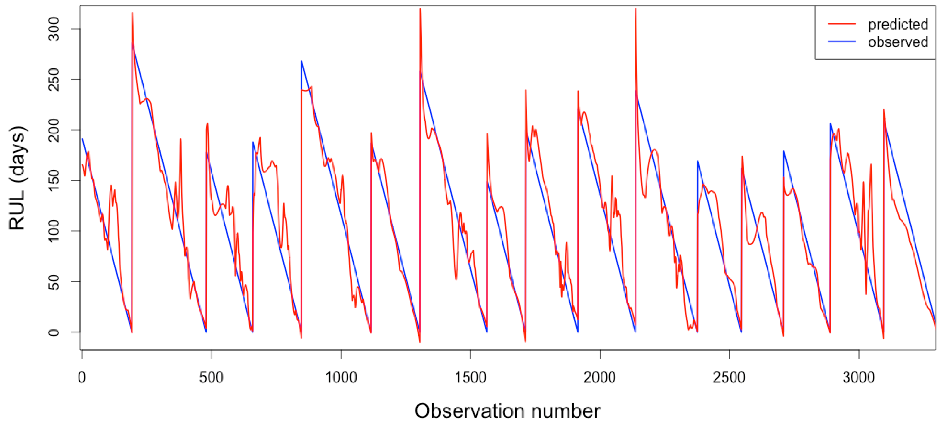
  • Firstly, the hypothesis that RUL diagnosis can be accurately modeled using a hybrid ABC–MARS-based model was confirmed. Indeed, a correlation coefficient equal to 0.92 was obtained when this hybrid ABC–SVM-based model with a radial basis function (RBF) as kernel was applied to experimental. Indeed, the predicted results for this model have been proved to be consistent with the observed RUL (see Figure 8).
  • Secondly, this study has developed a hybrid ABC–MARS-based model in which ABC technique was used to optimize the hyperparameters corresponding to the best MARS model for the RUL prediction from the other measured quality variables with success, in order to lower costs in the prediction of RUL.
  • Finally, another additional contribution of this research work was how the parameters setting of the MARS approach in the RUL regression affects the performance. From the obtained predicted results for the RUL, we can suggest the use of the MARS approach in combination with ABC technique for predicting the RUL values on account of its superior generalization capability compared to traditional regression techniques. The results verify that the ABC–MARS regression method significantly improves the generalization capability achievable with only the MARS-based regressor.
In summary, this innovative methodology could be applied to other sets of turbines with success. Additionally, authors of this research work have confidence that the results obtained in this study will be useful to promote new future research works in this direction.

Acknowledgments

The authors wish to acknowledge the computational support provided by the Department of Mathematics at University of Oviedo. Finally, we would like to thank Anthony Ashworth for his revision of English grammar and spelling of the manuscript.

Author Contributions

Paulino José García Nieto conceived and designed the experiments; Esperanza García-Gonzalo and Paulino José García Nieto built the mathematical model and solved the governing equations; Paulino José García Nieto and Esperanza García-Gonzalo performed the numerical experiments; and Paulino José García Nieto, Esperanza García-Gonzalo, Marta Menéndez Fernández and Antonio Bernardo Sánchez wrote the paper.

Conflicts of Interest

The authors declare no conflict of interest.

Appendix

Table A1 shows below a list of 139 main basis functions for the fitted ABC–MARS-based model and their coefficients, respectively. Please note that h ( x ) = x if x > 0 and h ( x ) = 0 if x 0 .
Table A1. List of basis functions of the best fitted ABC–MARS-based model for the RUL and their coefficients c i .
B i Definition c i
B 1 124.0
B 2 h(1597.13 T_HPC)−38
B 3 h(T_HPC 1597.13)−3
B 4 h(2388.1 F_sp)3181
B 5 h(2388.12 C_fsp)−3337
B 6 h(C_fsp 2388.12)118
B 7 h(T_LPC 642.787) × h(LPT_cb 23.2394)−1850
B 8 h(1597.13 T_HPC) × h(T_LPT 1406.23)−6
B 9 h(1597.13 T_HPC) × h(TP_HPC 554.245)−19
B 11 h(1597.13 T_HPC) × h(554.245 TP_HPC)8
B 11 h(1587.11 T_HPC) × h(2388.1 F_sp)−1056
B 12 h(T_HPC 1587.11) × h(2388.1 F_sp)1069
B 11 h(1597.13 T_HPC) × h(SP_HPC 47.3243)79
B 12 h(1597.13 T_HPC) × h(47.3243 SP_HPC)−66
B 13 h(1597.13 T_HPC) × h(R_ff 522.297)−118
B 14 h(1597.13 T_HPC) × h(522.297 R_ff)63
B 15 h(1590.19 T_HPC) × h(2388.12 C_fsp)1426
B 16 h(T_HPC 1590.19) × h(2388.12 C_fsp)−984
B 17 h(1597.13 T_HPC) × h(C_fsp 2388.12)−249
B 18 h(1597.13 T_HPC) × h(2388.12 C_fsp)−243
B 19 h(1597.13 T_HPC) × h(LPT_cb 23.3384)253
B 20 h(1597.13 T_HPC) × h(23.3384 LPT_cb)440
B 21 h(1399.42 T_LPT) × h(2388.12 C_fsp)−158
B 22 h(T_LPT 1399.42) × h(2388.12 C_fsp)560
B 23 h(TP_HPC 552.966) × h(F_sp 2388.1)3728
B 24 h(553.367 TP_HPC) × h(C_fsp 2388.12)−94
B 25 h(TP_HPC 553.367) × h(C_fsp 2388.12)194,839
B 26 h(2388.1 F_sp) × h(R_ff 522.264)4672
B 27 h(2388.1 F_sp) × h(522.264 R_ff)−10,382
B 28 h(2388.1 F_sp) × h(C_fsp 2388.04)37,628
B 29 h(2388.1F_sp) × h(LPT_cb 23.3955)32,232
B 30 h(642.298 T_LPC) × h(1597.13 T_HPC) × h(1406.23 T_LPT)−2
B 31 h(T_LPC 642.298) × h(1597.13 T_HPC) × h(1406.23 T_LPT)8
B 32 h(642.787 T_LPC) × h(1597.13 T_HPC) × h(SP_HPC 47.3243)−604
B 33 h(T_LPC 642.787) × h(1597.13 T_HPC) × h(SP_HPC 47.3243)−138
B 34 h(642.787 T_LPC) × h(B_e 393.013) × h(LPT_cb 23.2394)2316
B 35 h(642.787 T_LPC) × h(393.013 B_e) × h(LPT_cb 23.2394)1673
B 36 h(1587.11 T_HPC) × h(T_LPT 1398.34) × h(2388.1 F_sp)99
B 37 h(1587.11 T_HPC) × h(1398.34 T_LPT) × h(2388.1 F_sp)−356
B 38 h(1587.11 T_HPC) × h(T_LPT 1402.38) × h(2388.1 F_sp)905
B 39 h(1597.13 T_HPC) × h(1406.23 T_LPT) × h(F_sp 2388.08)187
B 40 h(1597.13 T_HPC) × h(1406.23 T_LPT) × h(2388.08 F_sp)129
B 41 h(1597.13 T_HPC) × h(1406.23 T_LPT) × h(SP_HPC 47.2194)−8
B 42 h(1597.13 T_HPC) × h(1406.23 T_LPT) × h(47.2194 SP_HPC)−9
B 43 h(1597.13 T_HPC) × h(T_LPT 1410.83) × h(SP_HPC 47.3243)13
B 44 h(1597.13 T_HPC) × h(1410.83 T_LPT) × h(SP_HPC 47.3243)−5
B 45 h(1597.13 T_HPC) × h(1406.23 T_LPT) × h(C_fsp 2388.05)52
B 46 h(1587.11 T_HPC) × h(TP_HPC 554.349) × h(2388.1 F_sp)1926
B 47 h(1587.11 T_HPC) × h(554.349 TP_HPC) × h(2388.1 F_sp)−1900
B 48 h(1597.13 T_HPC) × h(553.358 TP_HPC) × h(SP_HPC 47.3243)153
B 49 h(1597.13 T_HPC) × h(TP_HPC 554.245) × h(B_e 391.853)−77
B 50 h(1597.13 T_HPC) × h(TP_HPC 554.245) × h(391.853 B_e)−51
B 51 h(1597.13 T_HPC) × h(TP_HPC 553.505) × h(23.3384 LPT_cb)236
B 52 h(1597.13 T_HPC) × h(554.245 TP_HPC) × h(LPT_cb 23.375)2360
B 53 h(1597.13 T_HPC) × h(554.245 TP_HPC) × h(23.375 LPT_cb)−399
B 54 h(1597.13 T_HPC) × h(F_sp 2388.01) × h(R_ff 522.297)8036
B 55 h(1597.13 T_HPC) × h(2388.01 F_sp) × h(R_ff 522.297)−643
B 56 h(1597.13 T_HPC) × h(F_sp 2388.08) × h(2388.12 C_fsp)−7110
B 57 h(1597.13 T_HPC) × h(2388.08 F_sp) × h(2388.12 C_fsp)−1875
B 58 h(T_HPC 1587.11) × h(2388.1 F_sp) × h(LPT_cb 23.3398)−17,936
B 59 h(1597.13 T_HPC) × h(F_sp 2388.06) × h(LPT_cb 23.3384)−11,761
B 60 h(1597.13 T_HPC) × h(2388.06 F_sp) × h(LPT_cb 23.3384)−11,664
B 61 h(1597.13 T_HPC) × h(SP_HPC 47.3243) × h(R_ff 521.611)533
B 62 h(1597.13 T_HPC) × h(SP_HPC 47.3243) × h(521.611 R_ff)−249
B 63 h(1597.13 T_HPC) × h(522.297 R_ff) × h(HPT_cb 38.894)−81
B 64 h(1597.13 T_HPC) × h(522.297 R_ff) × h(38.894 HPT_cb)74
B 65 h(1597.13 T_HPC) × h(R_ff 522.315) × h(LPT_cb 23.3384)261
B 66 h(1597.13 T_HPC) × h(522.315 R_ff) × h(LPT_cb 23.3384)164
B 67 h(1597.13 T_HPC) × h(By_r 8.41459) × h(LPT_cb 23.3384)−23,851
B 68 h(1597.13 T_HPC) × h(B_e 392.68) × h(LPT_cb 23.3384)5485
B 69 h(1597.13 T_HPC) × h(392.68 B_e) × h(LPT_cb 23.3384)98
B 70 h(1399.42 T_LPT) × h(SP_HPC 47.1847) × h(2388.12 C_fsp)−16,641
B 71 h(1399.42 T_LPT) × h(47.1847 SP_HPC) × h(2388.12 C_fsp)5308
B 72 h(1399.42 T_LPT) × h(2388.12 C_fsp) × h(By_r 8.39473)17,357
B 73 h(TP_HPC 553.934) × h(2388.1 F_sp) × h(C_fsp 2388.04)−539,229
B 74 h(2388.1 F_sp) × h(C_fsp 2388.04) × h(HPT_cb 38.8679)−1,599,185
B 75 h(2388.1 F_sp) × h(C_fsp 2388.04) × h(LPT_cb 23.3088)649,885
B 76 h(642.298 T_LPC) × h(1597.13 T_HPC) × h(1406.23 T_LPT) × h(B_e 392.1)55
B 77 h(642.298 T_LPC) × h(1597.13 T_HPC) × h(1406.23 T_LPT) × h(392.1 B_e)2
B 78 h(T_LPC 642.298) × h(1597.13 T_HPC) × h(1406.23 T_LPT) × h(F_sp 2388.06)−960
B 79 h(T_LPC 642.298) × h(1597.13 T_HPC) × h(1406.23 T_LPT) × h(2388.06 F_sp)−418
B 80 h(T_LPC 642.298) × h(1597.13 T_HPC) × h(1406.23 T_LPT) × h(R_ff 521.725)20
B 81 h(T_LPC 642.298) × h(1597.13 T_HPC) × h(1406.23 T_LPT) × h(521.725 R_ff)165
B 82 h(T_LPC 642.298) × h(1597.13 T_HPC) × h(1406.23 T_LPT) × h(B_e 392.604)−44
B 83 h(T_LPC 642.298) × h(1597.13 T_HPC) × h(1406.23 T_LPT) × h(392.604 B_e)20
B 84 h(642.787 T_LPC) × h(T_HPC 1584.11) × h(TP_HPC 554.005) × h(LPT_cb 23.2394)−210
B 85 h(642.787 T_LPC) × h(T_HPC 1584.11) × h(554.005 TP_HPC) × h(LPT_cb 23.2394)1848
B 86 h(642.787 T_LPC) × h(1597.13 T_HPC) × h(SP_HPC 47.3243) × h(B_e 392.72)197
B 87 h(642.787 T_LPC) × h(1597.13 T_HPC) × h(SP_HPC 47.3243) × h(392.72 B_e)−407
B 88 h(642.787 T_LPC) × h(T_HPC 1584.11) × h(522.147 R_ff) × h(LPT_cb 23.2394)1530
B 89 h(642.787 T_LPC) × h(T_HPC 1584.11) × h(By_r 8.4459) × h(LPT_cb 23.2394)211,345
B 90 h(642.787 T_LPC) × h(T_HPC 1588.92) × h(393.013 B_e) × h(LPT_cb 23.2394)−6066
B 91 h(642.787 T_LPC) × h(1588.92 T_HPC) × h(393.013 B_e) × h(LPT_cb 23.2394)−247
B 92 h(T_LPC 642.15) × h(2388.1 F_sp) × h(C_fsp 2388.04) × h(LPT_cb 23.3088)23,278,307
B 93 h(T_LPC 642.39) × h(2388.1 F_sp) × h(C_fsp 2388.04) × h(LPT_cb 23.3088)−21,335,093
B 94 h(1597.13 T_HPC) × h(T_LPT 1401.3) × h(554.245 TP_HPC) × h(LPT_cb 23.375)7823
B 95 h(T_HPC 1587.11) × h(T_LPT 1402.61) × h(2388.1 F_sp) × h(LPT_cb 23.3398)−76,722
B 96 h(1597.13 T_HPC) × h(1406.23 T_LPT) × h(SP_HPC 47.326) × h(2388.05 C_fsp)2947
B 97 h(1597.13 T_HPC) × h(1406.23 T_LPT) × h(C_fsp 2388.05) × h(HPT_cb 38.931)1070
B 98 h(1597.13 T_HPC) × h(1406.23 T_LPT) × h(C_fsp 2388.05) × h(38.931 HPT_cb)1091
B 99 h(1597.13 T_HPC) × h(T_LPT 1404.49) × h(392.68 B_e) × h(LPT_cb 23.3384)−10,156
B 100 h(T_HPC 1587.11) × h(TP_HPC 553.743) × h(2388.1 F_sp) × h(LPT_cb 23.3398)60,136
B 101 h(1597.13 T_HPC) × h(TP_HPC 554.245) × h(F_sp 2387.99) × h(B_e 391.853)15,571
B 102 h(1597.13 T_HPC) × h(TP_HPC 554.056) × h(522.297 R_ff) × h(HPT_cb 38.894)706
B 103 h(1597.13 T_HPC) × h(554.056 TP_HPC) × h(522.297 R_ff) × h(HPT_cb 38.894)1170
B 104 h(1597.13 T_HPC) × h(553.505 TP_HPC) × h(HPT_cb 38.7938) × h(23.3384 LPT_cb)9516
B 105 h(1597.13 T_HPC) × h(553.505 TP_HPC) × h(38.7938 HPT_cb) × h(23.3384 LPT_cb)−882
B 106 h(1597.13 T_HPC) × h(F_sp 2388.13) × h(522.297 R_ff) × h(38.894 HPT_cb)686
B 107 h(1597.13 T_HPC) × h(2388.13 F_sp) × h(522.297 R_ff) × h(38.894 HPT_cb)−1888
B 108 h(T_HPC 1585.11) × h(2388.1 F_sp) × h(C_fsp 2388.04) × h(LPT_cb 23.3088)−1,906,032
B 109 h(T_HPC 1586.75) × h(2388.1 F_sp) × h(C_fsp 2388.04) × h(LPT_cb 23.3088)3,083,141
B 110 h(1597.13 T_HPC) × h(522.297 R_ff) × h(By_r 8.4177) × h(HPT_cb 38.894)54,655
B 111 h(1597.13 T_HPC) × h(R_ff 522.42) × h(392.68 B_e) × h(LPT_cb 23.3384)395
B 112 h(T_LPC 642.15) × h(2388.1 F_sp) × h(C_fsp 2388.04) × h(LPT_cb 23.3088)23,278,307
B 113 h(T_LPC 642.39) × h(2388.1 F_sp) × h(C_fsp 2388.04) × h(LPT_cb 23.3088)−21,335,093
B 114 h(1597.13 T_HPC) × h(T_LPT 1401.3) × h(554.245 TP_HPC) × h(LPT_cb 23.375)7823
B 115 h(T_HPC 1587.11) × h(T_LPT 1402.61) × h(2388.1 F_sp) × h(LPT_cb 23.3398)−76,722
B 116 h(1597.13 T_HPC) × h(1406.23 T_LPT) × h(SP_HPC 47.326) × h(2388.05 C_fsp)2947
B 117 h(1597.13 T_HPC) × h(1406.23 T_LPT) × h(C_fsp 2388.05) × h(HPT_cb 38.931)1070
B 118 h(1597.13 T_HPC) × h(1406.23 T_LPT) × h(C_fsp 2388.05) × h(38.931 HPT_cb)1091
B 119 h(1597.13 T_HPC) × h(T_LPT 1404.49) × h(392.68 B_e) × h(LPT_cb 23.3384)−10156
B 120 h(T_HPC 1587.11) × h(TP_HPC 553.743) × h(2388.1 F_sp) × h(LPT_cb 23.3398)60,136
B 121 h(1597.13 T_HPC) × h(TP_HPC 554.245) × h(F_sp 2387.99) × h(B_e 391.853)15,571
B 122 h(1597.13 T_HPC) × h(TP_HPC 554.056) × h(522.297 R_ff) × h(HPT_cb 38.894)706
B 123 h(1597.13 T_HPC) × h(554.056 TP_HPC) × h(522.297 R_ff) × h(HPT_cb 38.894)1170
B 124 h(1597.13 T_HPC) × h(553.505 TP_HPC) × h(HPT_cb 38.7938) × h(23.3384 LPT_cb)9516
B 125 h(1597.13 T_HPC) × h(553.505 TP_HPC) × h(38.7938 HPT_cb) × h(23.3384 LPT_cb)−882
B 126 h(1597.13 T_HPC) × h(F_sp 2388.13) × h(522.297 R_ff) × h(38.894 HPT_cb)686
B 127 h(1597.13 T_HPC) × h(2388.13 F_sp) × h(522.297 R_ff) × h(38.894 HPT_cb)−1888
B 128 h(T_HPC 1585.11) × h(2388.1 F_sp) × h(C_fsp 2388.04) × h(LPT_cb 23.3088)−1,906,032
B 129 h(T_HPC 1586.75) × h(2388.1 F_sp) × h(C_fsp 2388.04) × h(LPT_cb 23.3088)3,083,141
B 130 h(1597.13 T_HPC) × h(522.297 R_ff) × h(By_r 8.4177) × h(HPT_cb 38.894)54,655
B 131 h(1597.13 T_HPC) × h(R_ff 522.42) × h(392.68 B_e) × h(LPT_cb 23.3384)395
B 132 h(1597.13 T_HPC) × h(522.42 R_ff) × h(392.68 B_e) × h(LPT_cb 23.3384)−712
B 133 h(1597.13 T_HPC) × h(522.297 R_ff) × h(38.894 HPT_cb) × h(LPT_cb 23.3154)13,920
B 134 h(1597.13 T_HPC) × h(522.297 R_ff) × h(38.894 HPT_cb) × h(23.3154 LPT_cb)805
B 135 h(TP_HPC 554.065) × h(2388.1 F_sp) × h(C_fsp 2388.04) × h(LPT_cb 23.3088)11,978,365
B 136 h(2388.1 F_sp) × h(R_ff 521.936) × h(C_fsp 2388.04) × h(LPT_cb 23.3088)12,019,857
B 137 h(2388.1 F_sp) × h(C_fsp 2388.04) × h(By_r 8.42486) × h(LPT_cb 23.3088)−805,713,430
B 138 h(2388.1 F_sp) × h(C_fsp 2388.04) × h(By_r 8.41503) × h(LPT_cb 23.3088)−337,807,089
B 139 h(2388.1 F_sp) × h(C_fsp 2388.04) × h(By_r 8.4216) × h(LPT_cb 23.3088)517,391,406

References

  1. El-Sayed, A.F. Aircraft Propulsion and Gas Turbine Engines; CRC Press: Boca Raton, FL, USA, 2008. [Google Scholar]
  2. Wild, T.; Sterkenburg, R. Aircraft Turbine Engines; Avotek Information Resources: New York, NY, USA, 2008. [Google Scholar]
  3. Treager, I. Aircraft Gas Turbine Engine Technology; McGraw-Hill Science: New York, NY, USA, 2002. [Google Scholar]
  4. Soares, C. Gas Turbines: A Handbook of Air, Land and Sea Applications; Butterworth-Heinemann: San Diego, CA, USA, 2008. [Google Scholar]
  5. Saravanamuttoo, H.I.H.; Rogers, G.F.C.; Cohen, H.; Straznicky, P.V. Gas Turbine Theory; Pearson Education: London, UK, 2009. [Google Scholar]
  6. Frederick, D.; De Castro, J.; Litt, J. User’s Guide for the Commercial Modular Aero-propulsion System Simulation (C-MAPSS); Technical Manual TM2007-215026; NASA/ARL: Cleveland, OH, USA, 2007. [Google Scholar]
  7. Vachtsevanos, G.; Lewis, F.; Roemer, M.; Hess, A.; Wu, B. Intelligent Fault Diagnosis and Prognosis for Engineering Systems; John Wiley & Sons: Hoboken, NJ, USA, 2006. [Google Scholar]
  8. Brotherton, T.; Jahns, G.; Jacobs, J.; Wroblewski, D. Prognosis of Faults in Gas Turbine Engines. In Proceedings of the 2000 IEEE Aerospace Conference, Big Sky, MT, USA, 25 March 2000; pp. 163–171.
  9. Goebel, K.; Qiu, H.; Eklund, N.; Yan, W. Modeling Propagation of Gas Path Damage. In Proceedings of the 2007 IEEE Aerospace Conference, Big Sky, MT, USA, 3–10 March 2007; pp. 1–8.
  10. Pecht, M.G. Prognostics and Health Management of Electronics; John Wiley & Sons: Hoboken, NJ, USA, 2008. [Google Scholar]
  11. Tang, S.; Yu, C.; Wang, X.; Guo, X.; Si, X. Remaining useful life prediction of lithium-ion batteries based on the Wiener process with measurement error. Energies 2014, 7, 520–547. [Google Scholar] [CrossRef]
  12. Zhao, M.; Tang, B.; Tan, Q. Bearing remaining useful life estimation based on time–frequency representation and supervised dimensionality reduction. Measurement 2016, 86, 41–55. [Google Scholar] [CrossRef]
  13. Son, J.; Zhou, S.; Sankavaram, C.; Du, X.; Zhang, Y. Remaining useful life prediction based on noisy condition monitoring signals using constrained Kalman filter. Reliab. Eng. Syst. Saf. 2016, 152, 38–50. [Google Scholar] [CrossRef]
  14. Kapur, K.C.; Pecht, M.G. Reliability Engineering; John Wiley & Sons: Hoboken, NJ, USA, 2014. [Google Scholar]
  15. Walsh, P.; Fletcher, P. Gas Turbine Performance; Wiley-Blackwell: Oxford, UK, 2008. [Google Scholar]
  16. Kulikov, G.G.; Thompson, H.A. Dynamic Modelling of Gas Turbines: Identification, Simulation, Condition Monitoring and Optimal Control; Springer: New York, NY, USA, 2010. [Google Scholar]
  17. Si, X.S.; Wang, W.; Hu, C.H.; Zhou, D.H. Remaining useful life estimation—A review on the statistical data driven approaches. Eur. J. Oper. Res. 2011, 213, 1–14. [Google Scholar] [CrossRef]
  18. Kalbfleisch, J.D.; Prentice, R.L. The Statistical Analysis of Failure Time Data; Wiley: New York, NY, USA, 2002. [Google Scholar]
  19. Lawless, J.F. Statistical Models and Methods for Lifetime Data; Wiley-Interscience: New York, NY, USA, 2002. [Google Scholar]
  20. Zio, E.; Di Maio, F. A data-driven fuzzy approach for predicting the remaining useful life in dynamic failure scenarios of a nuclear system. Reliab. Eng. Syst. Saf. 2010, 95, 49–57. [Google Scholar] [CrossRef] [Green Version]
  21. Ahmadzadeh, F.; Lundberg, J. Remaining useful life prediction of grinding mill liners using an artificial neural network. Miner. Eng. 2007, 53, 1–8. [Google Scholar] [CrossRef]
  22. Friedman, J.H. Multivariate adaptive regression splines. Ann. Stat. 1991, 19, 1–141. [Google Scholar] [CrossRef]
  23. Sekulic, S.S.; Kowalski, B.R. MARS: A tutorial. J. Chemometr. 1992, 6, 199–216. [Google Scholar] [CrossRef]
  24. Friedman, J.H.; Roosen, C.B. An introduction to multivariate adaptive regression splines. Stat. Methods Med. Res. 1995, 4, 197–217. [Google Scholar] [CrossRef] [PubMed]
  25. Vapnik, V. Statistical Learning Theory; Wiley-Interscience: New York, NY, USA, 1998. [Google Scholar]
  26. Hastie, T.; Tibshirani, R.; Friedman, J.H. The Elements of Statistical Learning; Springer-Verlag: New York, NY, USA, 2003. [Google Scholar]
  27. Xu, Q.S.; Daszykowski, M.; Walczak, B.; Daeyaert, F.; de Jonge, M.R.; Heeres, J.; Koymans, L.M.H.; Lewi, P.J.; Vinkers, H.M.; Janssen, P.A.; et al. Multivariate adaptive regression splines—Studies of HIV reverse transcriptase inhibitors. Chemometr. Intell. Lab. Syst. 2004, 72, 27–34. [Google Scholar] [CrossRef]
  28. Karaboga, D.; Basturk, B. A powerful and efficient algorithm for numerical function optimization: Artificial bee colony (ABC) algorithm. J. Glob. Optim. 2007, 39, 459–471. [Google Scholar] [CrossRef]
  29. Eberhart, R.C.; Shi, Y.; Kennedy, J. Swarm Intelligence; Morgan Kaufmann: San Francisco, CA, USA, 2001. [Google Scholar]
  30. Clerc, M.; Kennedy, J. The particle swarm—Explosion, stability, and convergence in a multidimensional complex space. IEEE Trans. Evolut. Comput. 2002, 6, 58–73. [Google Scholar] [CrossRef]
  31. Olsson, A.E. Particle Swarm Optimization: Theory, Techniques and Applications; Nova Science Publishers: New York, NY, USA, 2011. [Google Scholar]
  32. Dorigo, M.; Stützle, T. Ant Colony Optimization; The MIT Press: Cambridge, MA, USA, 2004. [Google Scholar]
  33. Simon, D. Evolutionary Optimization Algorithms; Wiley: New York, NY, USA, 2013. [Google Scholar]
  34. Yang, X.-S.; Cui, Z.; Xiao, R.; Gandomi, A.H.; Karamanoglu, M. Swarm Intelligence and Bio-Inspired Computation: Theory and Applications; Elsevier: London, UK, 2013. [Google Scholar]
  35. Chou, S.-M.; Lee, S.-M.; Shao, Y.E.; Chen, I.-F. Mining the breast cancer pattern using artificial neural networks and multivariate adaptive regression splines. Expert Syst. Appl. 2004, 27, 133–142. [Google Scholar] [CrossRef]
  36. De Cos Juez, F.J.; Sánchez Lasheras, F.; García Nieto, P.J.; Suárez Suárez, M.A. A new data mining methodology applied to the modelling of the influence of diet and lifestyle on the value of bone mineral density in post-menopausal women. Int. J. Comput. Math. 2009, 86, 1878–1887. [Google Scholar] [CrossRef]
  37. García Nieto, P.J.; Martínez Torres, J.; de Cos Juez, F.J.; Sánchez Lasheras, F. Using multivariate adaptive regression splines and multilayer perceptron networks to evaluate paper manufactured using Eucalyptus globulus. Appl. Math. Comput. 2012, 219, 755–763. [Google Scholar] [CrossRef]
  38. García Nieto, P.J.; Álvarez Antón, J.C. Nonlinear air quality modeling using multivariate adaptive regression splines in Gijón urban area (Northern Spain) at local scale. Appl. Math. Comput. 2014, 235, 50–65. [Google Scholar] [CrossRef]
  39. García Nieto, P.J.; Sánchez Lasheras, F.; de Cos Juez, F.J.; Alonso Fernández, J.R. Study of cyanotoxins presence from experimental cyanobacteria concentrations using a new data mining methodology based on multivariate adaptive regression splines in Trasona reservoir (Northern Spain). J. Hazard. Mater. 2011, 195, 414–421. [Google Scholar] [CrossRef] [PubMed]
  40. García Nieto, P.J.; Alonso Fernández, J.R.; Sánchez Lasheras, F.; de Cos Juez, F.J.; Díaz Muñiz, C. A new improved study of cyanotoxins presence from experimental cyanobacteria concentrations in the Trasona reservoir (Northern Spain) using the MARS technique. Sci. Total Environ. 2012, 430, 88–92. [Google Scholar] [CrossRef] [PubMed]
  41. Zhang, W.G.; Goh, A.T.C. Multivariate adaptive regression splines for analysis of geotechnical engineering systems. Comput. Geotech. 2013, 48, 82–95. [Google Scholar] [CrossRef]
  42. Saxena, A.; Goebel, K.; Simon, D.; Eklund, N. Damage Propagation Modeling for Aircraft Engine Run-to-failure Simulation. In Proceedings of the 2008 IEEE International Conference on Prognostics and Health Management (PMH 2008), Denver, CO, USA, 6–9 October 2008; pp. 1–9.
  43. Wang, T.; Yu, J.; Siegel, D.; Lee, J. A Similarity-based Prognostics Approach for Remaining Useful Life Estimation of Engineered Systems. In Proceedings of the 2008 IEEE International Conference on Prognostics and Health Management (PMH 2008), Denver, CO, USA, 6–9 October 2008; pp. 1–6.
  44. Sun, J.; Zuo, H.; Wang, W.; Pecht, M.G. Application of a state space modeling technique to system prognostics based on a health index for condition-based maintenance. Mech. Syst. Signal Proc. 2012, 28, 585–596. [Google Scholar] [CrossRef]
  45. Wasserman, L. All of Statistics: A Concise Course in Statistical Inference; Springer: New York, NY, USA, 2003. [Google Scholar]
  46. Freedman, D.; Pisani, R.; Purves, R. Statistics; W.W. Norton & Company: New York, NY, USA, 2007. [Google Scholar]
  47. Ranganai, E. Quality of fit measurement in regression quantiles: An elemental set method approach. Stat. Probabil. Lett. 2016, 111, 18–25. [Google Scholar] [CrossRef]
  48. Picard, R.; Cook, D. Cross-validation of regression models. J. Am. Stat. Assoc. 1984, 79, 575–583. [Google Scholar] [CrossRef]
  49. Barnes, J.P.; Johnston, P.R. Application of robust Generalised Cross-Validation to the inverse problem of electrocardiology. Comput. Biol. Med. 2016, 69, 213–225. [Google Scholar] [CrossRef] [PubMed]
  50. Milborrow, S. Earth: Multivariate Adaptive Regression Spline Models, R Package, version 3.2–7; R Foundation for Statistical Computing: Vienna, Austria, 2014. [Google Scholar]
  51. Vega Yong, G.; Muñoz, E. ABCoptim: Implementation of Artificial Bee Colony (ABC) Optimization, R Package, version 0.13.11; R Foundation for Statistical Computing: Vienna, Austria, 2013. [Google Scholar]
Figure 1. Simplified diagram of the engine simulated (LPC: low pressure compressor; HPC: high pressure compressor; N1: turbine shaft; N2: turbine axis; LPT: low pressure turbine; and HPT: high pressure turbine).
Energies 09 00409 g001
Figure 2. Layout showing various modules and their connections as modeled in the simulation.
Energies 09 00409 g002
Figure 3. Correlation matrix of this problem with the two discarded independent variables: Physical core speed (C_sp) and Corrected core speed (C_csp).
Energies 09 00409 g003
Figure 4. Independent variables vs. dependent variable (RUL) for turbine 4. This turbine contains 189 observations for each variable (red line represents the fitted third degree polynomial or cubic polynomial).
Energies 09 00409 g004aEnergies 09 00409 g004b
Figure 5. A graphical representation of a spline basis function. The left spline ( x < t , ( x t ) ) is shown as a dashed line; and the right spline ( x > t , + ( x t ) ) as a solid line.
Energies 09 00409 g005
Figure 6. Relation between the fitness of a food source and objective function.
Energies 09 00409 g006
Figure 7. Flowchart of the hybrid ABC–MARS-based model.
Energies 09 00409 g007
Figure 8. Comparison between the remaining useful life observed and predicted by the hybrid ABC–MARS-based model for aircraft engines (r = 0.92) for the first 3200 observations.
Energies 09 00409 g008
Table 1. MAPSS input variables of the simulated engine to simulate the remaining useful life (RUL) with their mean and standard deviation.
Input VariablesSymbolMeanStandard Deviation
Total temperature at fan inlet (°R)T_f 5.19 × 10 2 6.54 × 10 11
Total temperature at LPC outlet (°R)T_LPC 6.43 × 10 2 5.00 × 10 1
Total temperature at HPC outlet (°R)T_HPC 1.59 × 10 3 6.13
Total temperature at LPT outlet (°R)T_LPT 1.41 × 10 3 9.00
Pressure at fan inlet (psia)P_f 1.46 × 10 1 3.39 × 10 12
Total pressure in bypass-duct (psia)TP_by 2.16 × 10 1 1.39 × 10 3
Total pressure at HPC outlet (psia)TP_HPC 5.53 × 10 2 8.85 × 10 1
Physical fan speed (rpm)F_sp 2.39 × 10 3 7.10 × 10 2
Physical core speed (rpm)C_sp 9.07 × 10 3 2.21 × 10 1
Engine pressure ratioE_pr1.30 4.66 × 10 13
Static pressure at HPC outlet (psia)SP_HPC 4.75 × 10 1 2.67 × 10 1
Ratio of fuel flow to Ps30 (pps/psi)R_ff 5.21 × 10 2 7.38 × 10 1
Corrected fan speed (rpm)C_fsp 2.39 × 10 3 7.19 × 10 2
Corrected core speed (rpm)C_csp 8.14 × 10 3 1.91 × 10 1
Bypass ratioBy_r8.44 3.75 × 10 2
Burner fuel-air ratioB_far 3.00 × 10 2 1.56 × 10 14
Bleed enthalpyB_e 3.93 × 10 2 1.55
Demanded fan speed (rpm)D_fsp 2.39 × 10 3 0.00
Demanded corrected fan speed (rpm)D_cfsp 1.00 × 10 2 0.00
HPT coolant bleed (lbm/s)HPT_cb 3.88 × 10 1 1.81 × 10 1
LPT coolant bleed (lbm/s)LPT_cb 2.33 × 10 1 1.08 × 10 1
Table 2. Initial ranges of the three hyperparameters of the ABC–MARS-based model fitted in this study.
MARS HyperparametersLower LimitUpper Limit
Maximum number of basis functions (MaxFuncs)3200
Penalty parameter (d)−14
Interactions14
Table 3. Optimal hyperparameters of the best-fitted MARS model found with the ABC technique.
HyperparameterValues of Optimal Hyperparameters
Maximum number of basis functions (MaxFuncs)164
Penalty parameter (d)2
Interactions4
Table 4. Significance ranking for the variables involved in the best fitted ABC–MARS-based model for the RUL prediction according to criteria Nsubsets, GCV and RSS.
Input VariableNsubsetsGCVRSS
T_HPC122100.0100.0
C_fsp12298.298.2
T_LPC12062.562.8
TP_HPC12062.562.8
F_sp12062.562.8
R_ff12062.562.8
LPT_cb12062.562.8
T_LPT11756.656.9
By_r11552.552.9
HPT_cb10946.146.5
B_e10643.844.3
SP_HPC10040.941.3

