Power Production Losses Study by Frequency Regulation in Weak-Grid-Connected Utility-Scale Photovoltaic Plants

Abstract

Nowadays, an increasing penetration of utility-scale photovoltaic plants (USPVPs) leads to a change in dynamic and operational characteristics of the power distribution system. USPVPs must help to maintain the system stability and reliability while implementing minimum technical requirements (MTRs) imposed by the utility grid. One of the most significant requirements is about frequency regulation (FR). Overall production of USPVPs is reduced significantly by applying FR curves, especially in weak grids with high rate of frequency faults. The introduction of a battery energy storage system (BESS) reduces losses and improves the grid system reliability. Experimental frequency and irradiance data of several weak grids have been used to analyse USPVPs losses related to FR requirements and benefits from the introduction of a BESS. Moreover, its economic viability is showen without the need for any economic incentives.

1. Introduction

An increasing penetration of utility-scale photovoltaic plants (USPVPs) in the overall electric system requires the maintenance of their system stability and reliability. The required actions are divided into three categories depending on the time scale of grid operation [1]. First, the faster technique (sub-seconds to minutes time scale) is related to the photovoltaic (PV) plant response to grid disturbances on the point of common coupling (PCC). The second is related to load balancing which is of the order of sub-hours to days, and is controlled by the utility-grid. The third action is about future electric systems designing (order of years). USPVPs on each of these categories have a different role and should be studied accordingly.

Countries around the world are demanding minimum technical requirements (MTRs) for USPVPs besides active contribution to grid stability and power quality [2,3,4,5,6,7], in order to comply with the first category of system stability actions. Requirements are not only under normal conditions but also under faulty conditions, such as low voltage, phase jump, under/over frequency, etc.

Unlike the inherent electromechanical dynamics of synchronous generators, PV generators’ response based on power electronics is quite different. It needs a special attention on the grid frequency stability control actions [8,9]. Frequency regulation (FR) techniques have been studied widely in the literature [1,9,10,11,12,13,14,15,16,17,18,19,20]. All FR methods require a reduction over the active power generation on USPVPs. Consequently, if MTRs about FR are fulfilled, the USPVPs will have to consider additional losses, and a reduction of the overall plant profit.

Figure 1 shows a recent literature classification of FR methods used on PV applications. Depending on the grid system size (microgrids or utility-scale grids), the problem will be resolved with different techniques [1].

PV microgrids methods are mainly allocated inside power converters. There are two options: an open loop active power versus frequency control, with a hysteresis droop curve, or a defined look-up table; or a control droop method over the active power reference, in order to emulate the characteristic of synchronous generators against frequency excursions. All of them have been applied widely for PV microgrids [9,13,14,15,16,17,18,19,20]. However, these techniques are not able to be applied on USPVPs, because the capacity of one inverter could not be enough to move the grid frequency [21,22].

Notice that USPVPs solutions have two main groups. On the one hand, local regulation is done with a local active power curtailment, in a function of measured frequency and defined by the right grid code [2,3,4,5,6,7]. On the other hand, power system resident techniques are based on setting an external curtailment on the converters [1]. The curtailment value could come from the utility grid or from an automatic gain controller (AGC). The AGC could be a centralized or a distributed one, with the same control signal for every unit or with an individual control for each unit, respectively. Additionally, AGC methods could combine curtailment actions controlling deloaded reserves or energy storage systems (ESS) for further functionalities.

MTRs for USPVPs describe power droop curtailment curves to help the system stability. Nevertheless, USPVPs cannot store by itself the remaining energy during a frequency disturbance. Consequently, FR techniques lead to production losses that must be considered. In strong grids, with a grid frequency value very stable, the problem is irrelevant because the occurrence of a fault during a year is very small [22,23]. However, in weak grids like Puerto Rico, Low California or the Sistema Interconectado Norte Grande (SING) in Chile, grid oscillations could vary significantly power production, and a comprehensive study of USPVP losses related to FR requirements is needed.

USPVPs are built with a lot of PV electronic power converters. Nowadays, PV power converters generation response is very fast [24,25]. Therefore, they could reduce USPVPs impact over electric weak grids. Worldwide utility grids have modified MTRs with harder time response requirements, in order to use the advantage of the new power converter abilities. Reducing time response not only reduces the USPVP impact over grid frequency, but also helps the grid frequency stability. This clearly is always achieved at the expense of a loss of energy injected. Consequently, PV investors have to take this effect into account to calculate the plant profitability.

The overall USPVP power output must remain according to MTRs, but additional systems could be installed to optimize the plant production. An ESS could be used to save the energy during fault events. Moreover, an ESS could be used to regulate other requirements such as ramp rates, curtailments, etc. [1]. The most popular technology for PV applications is a battery energy storage system (BESS) [13,14,15,16,17,18,19,20,21,22,23,26,27,28,29].

However, BESS prices are too high. Therefore, legislation of California, New York, Hawaii and Germany amongst others, provide BESS economic incentives [30,31,32,33]. The objective is to help the installation of new BESS, that otherwise would not be profitable. This paper shows some real cases where the installation of a BESS is justified without any need for economic incentives, and reduces the installation price kWh.

This manuscript is organized as follows: Section 2 gives a review of international MTRs about FR. Section 3 describes the electric grid frequency behaviour, PV modelling, and expected power generation. Section 4 provides experimental test results about expected generation losses. Section 5 provides possible performance scenarios by introducing an ESS. Finally, discussions are given in Section 6.

2. Frequency Regulation

2.1. Grid Code Requirements

Despite grid code harmonization being desirable, local grid conditions lead to local grid requirements defined for every country.

Table 1. FR utility-scale photovoltaic plants (USPVPs) minimum technical requirements (MTRs) review. FRT: frequency ride through; BDEW: German association of energy and water industries; CEI: Electrotechnical Italian Committee; NERSA: National energy regulator of South Africa; CFE: Comisión Federal de Electricidad; PREPA: Puerto Rico Electric Power Authority; CNE: National Commission of Energy.

Country	FRT	FR
Germany (BDEW)
Italy (CEI)
South Africa (NERSA)
Mexico (CFE)
Puerto Rico (PREPA)
Chile (CNE)

shows recently published frequency ride through (FRT) and FR requirements [2,3,4,5,6,7]. On the one hand, FRTs set some thresholds to limit the converters frequency operation range. If the frequency reaches the limit after a defined time, the unit will be disconnected to prevent damage to the equipment. On the other hand, FR curves are pointed out. So, the power will be reduced applying a defined droop imposed by each country legislation.

German and Italian legislations describe the classical droop curve. FR techniques apply when a starting frequency is passed (50.2 Hz for German code). Then a droop factor reduces the active output power of the plant with respect to the active output power previous to the beginning of the fault condition ($P_{\mathrm{M}}$). However, if the frequency is partially restored, the droop factor continues on his lowest value. The droop factor is cancelled only when the frequency recovers to nearly the nominal grid frequency value (50.05 Hz for German code).

Other grid codes such as Mexico and Puerto Rico are not related to $P_{\mathrm{M}}$. Instead of that, they define an increment related to the nominal power plant capacity $\Delta P/P_{\mathrm{n}}$.

Puerto Rico, Mexico and South Africa requirements look alike for over-frequencies, but establish special requirements for under-frequencies. Hysteresis curves, and the nominal output power of the plant ($P_{\mathrm{n}}$) instead of $P_{\mathrm{M}}$ are the main differences for over-frequencies faults behaviour. However, for under-frequencies, a deload reserve or an ESS is required, in order to increase the maximum available power of the plant ($P_{\text{ava}}$). South African frequencies are pointed out with labels from $f_1$ to $f_6$. $f_2$ and $f_3$ point out the thresholds to begin the FR action for under-frequencies and over-frequencies, respectively. $f_1$ and $f_4$ point out the frequency magnitude to saturate the frequency droop curve to $P_{\text{ava}}$ or the minimum required ($P_{\text{min}}$), for under-frequencies and over-frequencies, respectively. Finally, $f_6$ points out the recovery frequency threshold.

Finally, Chilean code is similar to German legislation, but FR recovery is not abrupt. However, the restoration is performed with the same frequency ramp than downwards, only it is timed to a maximum of 0.2 p.u./min.

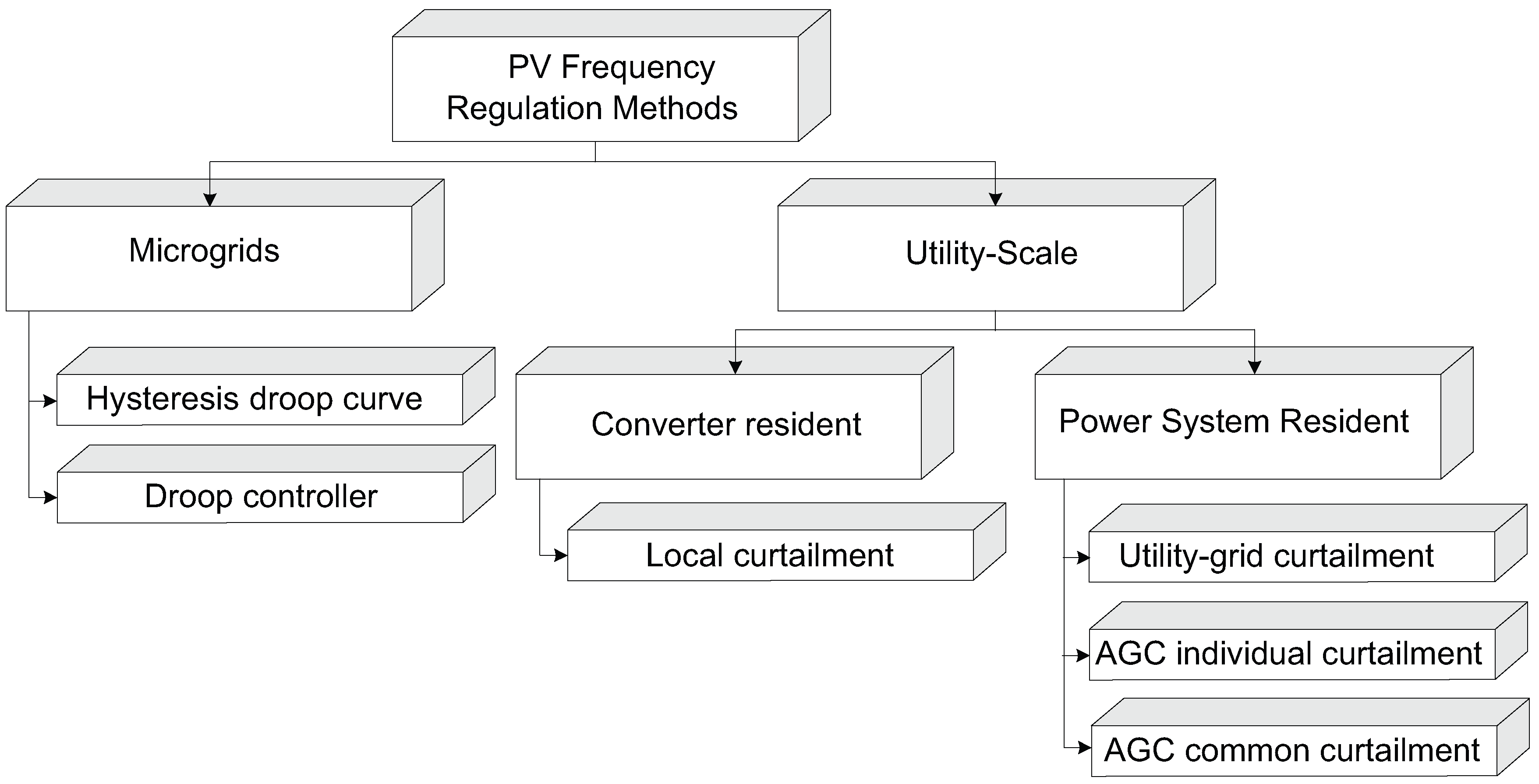
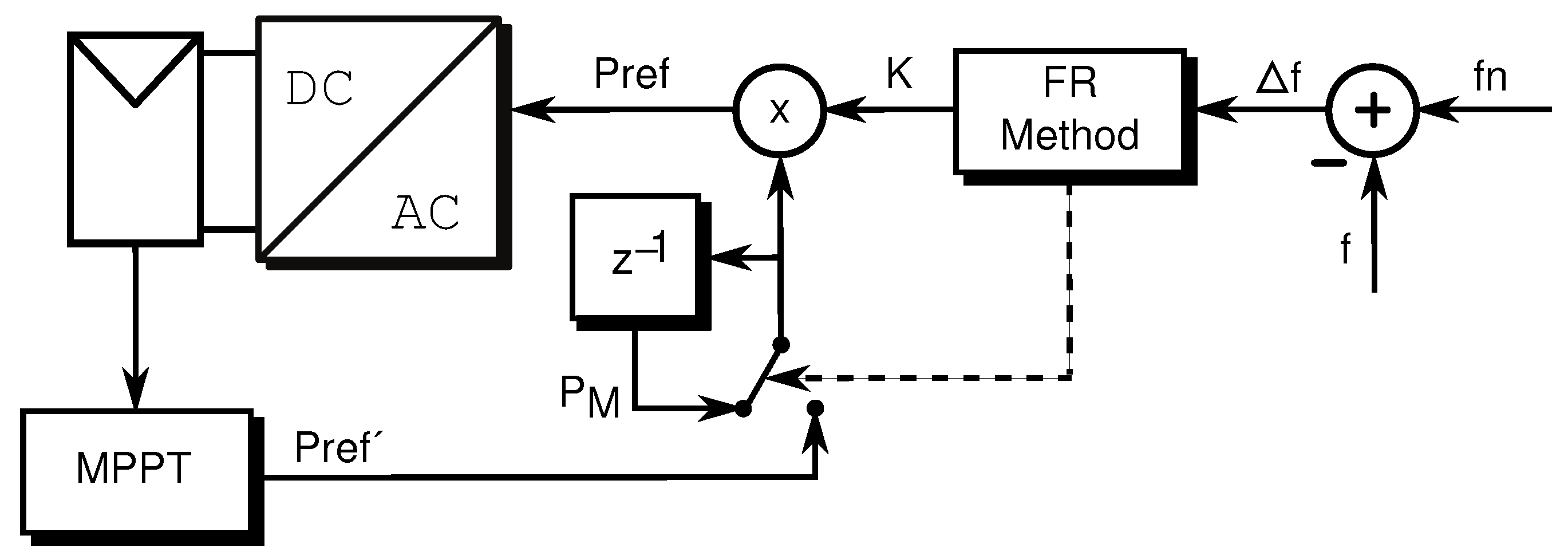
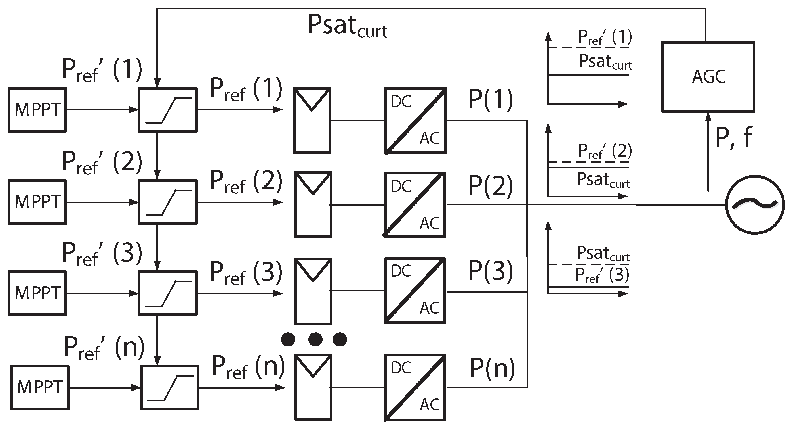
2.2. Frequency Regulation Methods

Figure 2 shows a typical PV converter control block diagram. The control scheme is divided into four layers: high, middle, low and hardware layer. FR capability for USPVPs is managed inside the middle layer, providing a suitable input data for the active power reference saturation threshold calculation. Typically, it could be performed locally or remotely. Remote active power saturation is set by $P_{{\text{sat}}_{\text{curt}}}$ signal, a power reference curtailment sent by the AGC. Local active power saturation is calculated inside the FR method block.

The converter resident method acts in function of the local data of the converter, providing a droop factor over the maximum power saturation value. The droop factor (K) could be referenced to the nominal converter power [6,7] ($P_{\mathrm{n}}$), or related to the active reference power previous to the frequency excursion [2,3,4,5] ($P_{\mathrm{M}}$). Figure 3 points out a typical block diagram control of the FR control scheme. Maximum power point tracker (MPPT) output reference ($P_{\text{ref}}$’) is modified by FR algorithm to provide a suitable current output power reference ($P_{\text{ref}}$).

The power system resident technique works in a similar way. However, every converter receives a curtailment saturation reference from an AGC ($P_{{\text{sat}}_{\text{curt}}}$), who calculates the right power saturation value. The curtailment signal is due to many factors, one of them, the FR control of the PPC (Figure 4). Each inverter has a different output power level but all of them have the same curtailment signal. As a result, each inverter could be saturated in a different way. For example, at Figure 4, unit 1 has decreased its power ($P\left(1\right)$)more than unit 2 power ($P\left(2\right)$), and unit 3 does not need to saturate its output ($P\left(3\right)$). But the power plant result will be the same that applying a converter resident solution.

2.3. Battery Energy Storage System Rule-Based Control

The BESS should operate according to a rule-based control in order to achieve its objective. Figure 5 shows the control law implemented in the BESS to get the results provided in this paper. The main objective of the BESS is to fulfil the mandatory FR MTRs.

The BESS power output ($P_{\text{BESS}}$) tries to provide the necessary FR active power contribution ($P_{\text{FR}}$), in order to minimize the USPVP losses. Therefore, there will be losses due to FR actions only when $P_{\text{FR}}$ is greater than the maximum active power capacity of the BESS ($P{\text{max}}_{\text{BESS}}$), or when the state of charge (SOC) of the BESS system exceeds the range of operation defined ($[SO{C}_{\text{min}},SO{C}_{\text{max}}]$). The efficiency of the BESS (${\mathsf{\eta }}_{\text{BESS}}$) has been considered to estimate the SOC correctly too.

If no FR action was required ($P_{\text{FR}}$ is zero), then a recovery process could be made. The objective is to charge or discharge the BESS to its initial state ($SO{C}_{\text{ini}}$). Therefore, the BESS could regain its full capacity to compensate any sub-frequency or over-frequency occurrence. Moreover, a slope is introduced in the $P_{\text{BESS}}$ reference calculation ($R_{\text{BESS}}$) to smooth the power output behaviour to the nominal power charging value ($R_{\mathrm{p}}$). Finally, $T_{\mathrm{s}}$ points out the sample time of the algorithm.

3. Frequency Regulation Behaviour Methods in Weak Grids

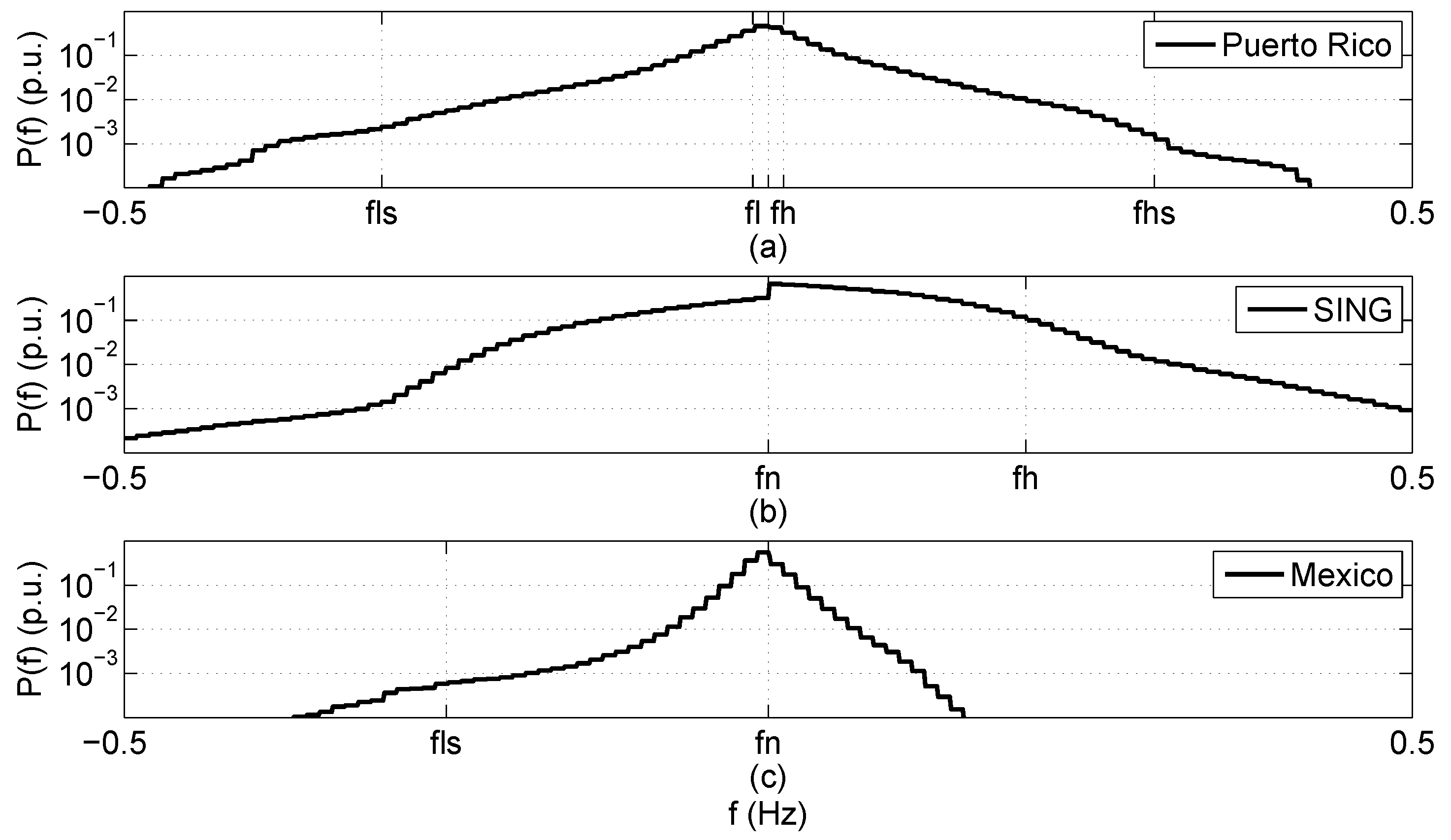
3.1. Weak Grids Frequency Excursions

A classical approach divides power grids into two parts: transmission lines and distribution lines [34]. On the one hand, transmission lines connect huge power production plants with consumption centres via high voltage links. On the other hand, distribution lines go to households and industry with medium and low voltage lines.

Weak grids have a relative small number of power sources and loads compare to a conventional national electric grid, so any unexpected change could produce voltage and frequency excursions. Consequently, these frequency excursions will lead the PV system to reduce its output production to comply with current MTRs.

In order to quantize the problem, frequency excursions have been analysed for three different weak power grids: Puerto Rico (Puerto Rico Electric Power Authority (PREPA)), Chile (SING), and Low California or Mexico (Comisión Federal de Electricidad (CFE)). At least 20 days have been analysed for every grid to get reliable results. A grid power analyser set in a PV power plant was used to record the frequency measurements in Puerto Rico and Low California. However, SING frequency data measurements were provided by the utility grid. For all cases, the time sample of the measurements was $4s$.

Figure 6 shows the time percentage in with a certain frequency value is over passed for these systems. In each graph, some key values are pointed out: the nominal frequency ($f_{\mathrm{n}}$); frequency threshold where the FR begins, $f_{\mathrm{l}}$ for sub-frequencies and $f_{\mathrm{h}}$ for over-frequencies; and frequency threshold where the FR ends, $f_{\text{sl}}$ for sub-frequencies and $f_{\text{sh}}$ for over-frequencies.

Note that every grid has different behaviours. The Puerto Rico probability disturbance spectra is almost symmetrical, SING has more over-frequency faults because there is over generation, and Low California has more sub-frequency faults because there is over consumption. In all cases, $f_{\mathrm{l}}$ and $f_{\mathrm{h}}$ thresholds are over-passed with an occurrence greater than $10\%$, so production losses are significant and an analysis is justified.

Moreover, Figure 7 shows how long the frequency excursions are. $T_{\text{max}}$ points out the longest clearing time registered for a certain frequency disturbance. For every grid, results are of the same magnitude, registering faults near 50 min duration at $f_{\mathrm{h}}$.

Figure 8 points out the mean clearing time $T_{\text{mn}}$ for such a disturbance. Note that the mean time of excursions after passing saturation thresholds ($f_{\text{hs}}$ and $f_{\text{ls}}$) goes up lightly. This is because the saturation of the FR droop control minimizes the restoration counter-effect of the method, incrementing the mean time of the perturbation.

Finally, Figure 9 and Figure 10 show the occurrence probability difference between day and night in the case of SING grid (Chile). Figure 9 shows a greater faulty condition at day-time than at night-time, so FR techniques over PV plants are plenty justified. Figure 10 shows more detail for the frequency value $f_{\mathrm{h}}$ with the hourly frequency disturbance occurrence probability. Shadowed parts are related to night time. Three relevant peaks are presented, and all three are in day-time.

Therefore, Figure 6 shows frequency behaviour for three remarked different types of weak grids. All cases show a high occurrence probability of frequency excursions compared to FR MTR thresholds, so an important decrease on PV power output is expected. Moreover, Figure 7 and Figure 8 point out significant frequency faults duration, so energy losses required to comply with MTRs will be very high and must be considered in the USPVP viability study.

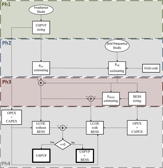
3.2. Utility-Scale PhotoVoltaic Plants Sizing

The availability of solar power sources must be considered. Production of a PV plant could be calculated from several environment measures. For example, a good approximation could be made with irradiance and temperature probes. The left side of Figure 11 shows typical irradiance curves of a solar plant in different weather seasons in the region of SING (Chile), and right side shows temperature measurements accordingly. The expected irradiance varies during the day. Moreover, the irradiance curve varies from summer to winter.

A correct sizing of a USPVP needs irradiance data from all seasons to have a complete spectra of solar profiles. Two different scenarios have been studied with real data from Copiapo (Chile) and Virgin Islands (next to Puerto Rico) [35] for a whole year of irradiance.

Copiapo irradiance and temperature measurements have been collected with sensors allocated inside a PV plant in Copiapo with a sample time of 2 s, and Virgin Islands data have been provided by NREL with a weather station with a sample time of 60 s.

Figure 12a shows Chilean irradiance measurements per month, marking the maximum, average and minimum measurements of the daily irradiation registered. Manufacturers usually establish a rule of thumb to sizing the maximum power capability of the power converters between $0.9$ and $0.75$ of the maximum averaged power expected for the irradiance measurements [36,37,38]. A division factor of $1.2$ over the maximum average irradiation registered has been considered. Figure 12c shows the averaged expected time per day to have the USPVP at full power in the Chilean case. Similarly, Figure 12b,d shows the same data for the Puerto Rican case.

Recently, several models have been developed to estimate the available power for USPVPs [39]. Wavelet variability model (WVM) is used strongly by engineers for sizing new USPVPs [40,41]. The algorithm provides an overall effective irradiance measure for all the plant.

Parameters used to get the WVM effective measurements have been set in accordance with USPVP characteristics, real location, and suggestions over the method [40,41].

Table 2. Wavelet variability model (WVM) settings.

Parameter	Chile	Puerto Rico
Power plant capacity	300 MW	300 MW
PV panels density	41 W/m${}^2$	41 W/m${}^2$
PV plant area	square	square
PV panels tilt	${27}^{\circ }$	${18}^{\circ }$
Cloud speed	10 m/s	10 m/s
Latitude	$-27.165661$	$18.059815$
Longitude	$-70.795136$	$-65.851908$

points out a list of parameters used for the estimation.

4. Frequency Regulation Results

USPVPs studied in Section 3 have been selected to perform an analysis about FR production losses. Experimental measurements of irradiance and grid frequency of SING (Chile) and Puerto Rico have been used to obtain results, using each grid code respectively [5,6].

Table 3. FR settings.

Parameter	Chile	Puerto Rico
Start droop over frequency ($f_{\mathrm{o}0}$)	50.2 Hz	60.012 Hz
Stop droop over frequency ($f_{\mathrm{o}1}$)	50.5–52 Hz	60.3 Hz
Maximum droop over frequency ($D_{\mathrm{o}}$)	1 p.u.	1 p.u.
Start droop under frequency ($f_{\mathrm{u}0}$)	N/A	59.988 Hz
Stop droop under frequency ($f_{\mathrm{u}1}$)	N/A	59.7 Hz
Maximum droop under frequency ($D_{\mathrm{u}1}$)	N/A	0.1 p.u.
Recovery ramp rate ($ram{p}_{\text{rec}}$)	0.2 p.u./s.	N/A

sets parameters of FR method for both experiments.

Figure 13 shows transient behaviour of one day at Copiapo (Chile). Both frequency and output power are plotted. Several curves are pointed out: the expected power generation without FR ($P_{\text{in}}$); and the real plant output applying three different scenarios for upper frequency $f_1=\{C_1,C_2,C_3\}=\{52,51,50.5\}$ Hz. All cases show significant reduction in power production, especially the hardest requirement in the case of the Chilean grid code, with power reductions of up to $75\%$ of active power.

The Puerto Rico grid code response has been analysed too. Real frequency and irradiation measurements have been taken into account. Figure 14 shows transient behaviour of one day at Puerto Rico. $10\%$ USPVP have been reserved for upper frequency excursions in order to comply with the Puerto Rican grid code. Again, Figure 14 points out transient frequency and power plant output.

Figure 14 shows several frequency peaks up to 60.3 Hz ($f_{\text{o1}}$), but the active power reduction is not as severe as in Chile because the FR is limited to 0.1 p.u. However, 0.1 p.u. of the solar plant must be reserved, increasing the total production losses.

4.1. Power Losses Applying Frequency Regulation

One day transient analysis of Figure 13 and Figure 14 were repeated for a whole month. Moreover, transient results have been obtained for different solar irradiance profiles. The same grid disturbances have been tested against several months of irradiance data, considering 31 and 20 days of frequency for Chile and Puerto Rico respectively.

Figure 15 and Figure 16 quantize the total energy losses due to FR techniques for Chilean and Puerto Rican grid code respectively. Case (a) shows daily energy losses ($e_{\text{loss}}$) and Case (c) shows daily remnant energy ($e_{\text{rem}}$). Both of them use real data acquisition from one month. Cases (b) and (d) show the evolution for several months of energy losses and mean remnant energy respectively. Chilean case shows a season dependency, but Puerto Rico holds the losses approximately constant. Both cases have significant losses registered up to 0.25 p.u.h/day and 0.5 p.u.h/day of the plant at full power. The introduction of an ESS could save part of this energy, increasing the production of the plant.

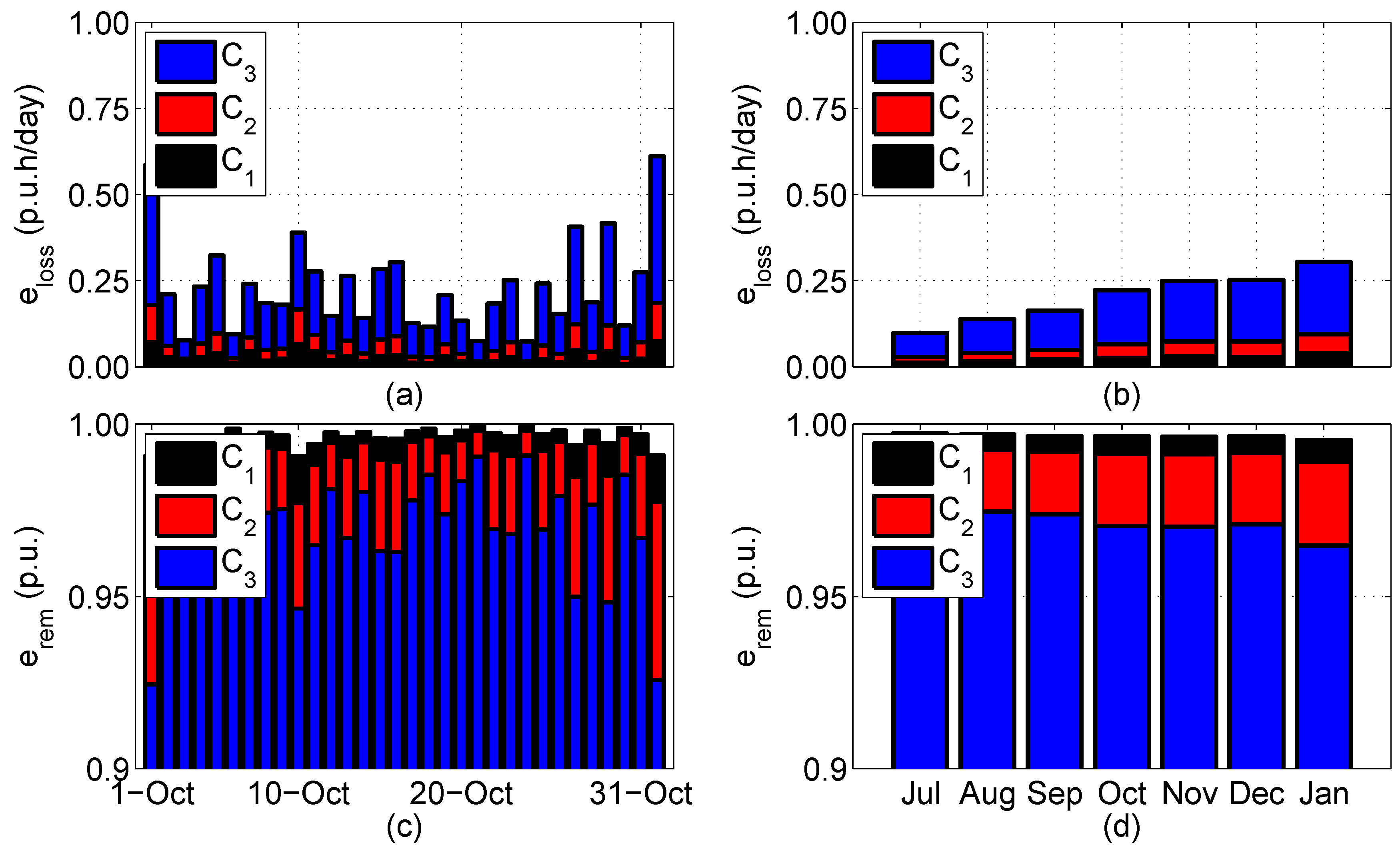
5. Battery Energy Storage System Results

The Puerto Rican grid code recommends at least the $10\%$ of USPVP nominal power output for the BESS peak power output [6]. Therefore, the BESS capacity allows the fulfilment of the required $10\%$ of reserve load. Consequently, BESS peak power has been set to $10\%$ of USPVP nominal power output for both scenarios.

Several BESS capacity scenarios have been studied.

Table 4. BESS settings: maximum charging active power ($C_{\mathrm{p}}$); maximum discharging active power ($D_{\mathrm{p}}$); recovery active power ($R_{\mathrm{p}}$); minimum allowed SOC ($SO{C}_{\text{min}}$); and overall efficiency of the BESS (${\mathsf{\eta }}_{\text{BESS}}$).

BESS Settings
Parameter	$C_{\mathbf{p}}$	$D_{\mathbf{p}}$	$R_{\mathbf{p}}$	$SO{C}_{\mathbf{m}\mathbf{i}\mathbf{n}}$	${\mathsf{\eta }}_{\mathbf{B}\mathbf{E}\mathbf{S}\mathbf{S}}$
Value	0.1 p.u.	0.1 p.u.	0.02 p.u.	0.2 p.u.	0.9 p.u.

shows the main parameters considered for the BESS. The values have been selected according to Chilean and Puerto Rican MTRs [5,6], and to manufacturer’s datasheets [42,43,44]. $C_{\mathrm{p}}$ and $D_{\mathrm{p}}$ are the maximum instantaneous active power to charge and discharge the battery respectively. If there was not any frequency disturbance, the battery would be charged or discharged to the BESS $SO{C}_{\text{ini}}$ at a defined active power rate ($R_{\mathrm{p}}$). $SO{C}_{\text{min}}$ is the minimum SOC allowed of the BESS, lower SOCs than $SO{C}_{\text{min}}$, which are not allowed because a big depth of discharge (DOD) reduces greatly the expected life of the battery. Finally, ${\mathsf{\eta }}_{\text{BESS}}$ points out the overall efficiency of the BESS, including the charging and discharging process.

Data from some manufacturers have been considered [42] to determine the BESS life expectancy under the working conditions. In fact, Figure 17 shows the expected battery number of cycles (NOC) $versus$ the load cycle DOD.

Finally, the levelized cost of electricity (LCOE) [45] is calculated for both scenarios (with and without BESS), in order to quantize the improvement by including a BESS.

5.1. Reducing Losses with Battery Energy Storage System

Figure 18 shows the response of Chilean USPVP with $f_1$ at 50.5 Hz for an BESS capacity (C) of 0.00277 p.u.h ($C_1$), 0.00833 p.u.h ($C_2$), and 0.015 p.u.h ($C_3$). Capacity magnitudes are related to the nominal output power of the USPVP. The introduction of the BESS reduces expected losses to less than the half previous case losses, even for small BESS capacity.

Moreover, Figure 19 shows results from similar experiments over Puerto Rican USPVP design scenario. The introduction of a BESS releases the reserved PV load, increasing the overall efficiency of the system up to $10\%$ of the total power plant production.

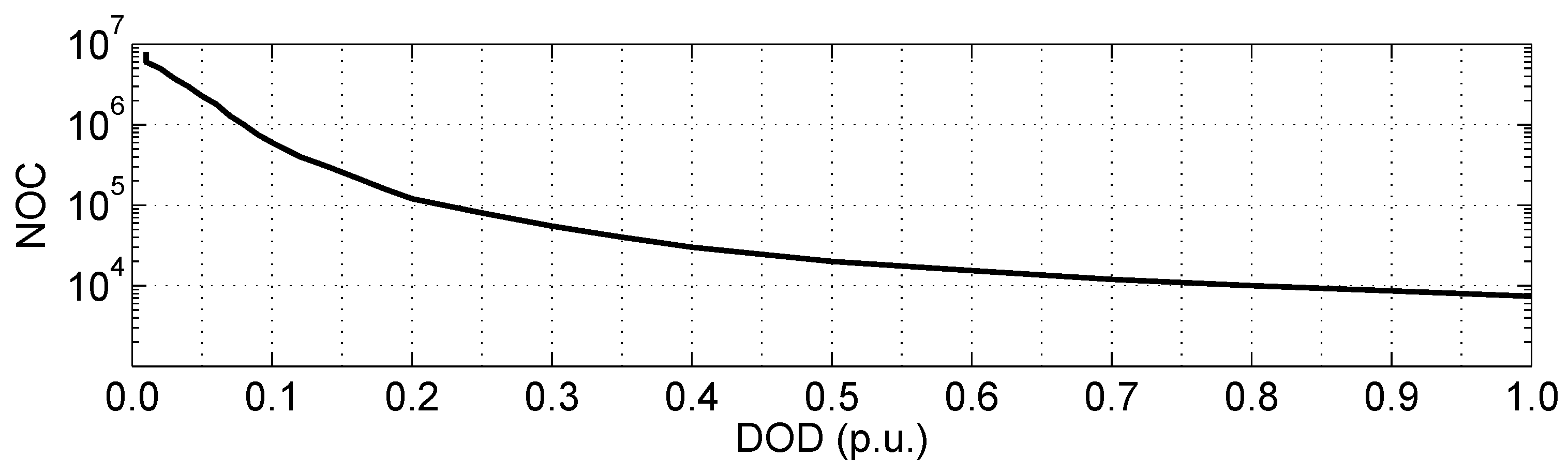
5.2. Battery Energy Storage System Life Cycle

The BESS life cycle is another important factor that must be taken into account when correctly sizing the BESS. Great charging/discharging cycles seriously reduce batteries life expectancy. However, BESS output must fulfil the required FR response with provided irradiance and frequency measurements. BESS capacity (C) has been tested for a wide range of values, getting expected losses and BESS life expectancy for all cases.

Figure 20 and Figure 21 show both expected losses and end of life (EOL) of BESS for Chilean and Puerto Rican cases. Above a certain value, increasing BESS capacity does not significantly reduce the energy losses of the whole system. However, the life expectancy could grow for several years, adding a little more capacity than the minimum required.

A typical value of EOL of a USPVP could be around 20 years. For example, in the Puerto Rican case, a capacity value of 0.025 p.u.h allows us to reach an EOL of 20 years. Figure 21 shows that the losses curve around C = 0.025 p.u.h is almost flat, so the selected C value could be a suitable one.

5.3. Levelized Cost of Electricity Estimation

LCOE is estimated for both cases: Puerto Rican and Chilean ($f_1$ = 50.5 Hz) plants. Two scenarios have been considered, with and without BESS, in order to quantize the difference between the two solutions.

Parameters have been selected according to previous sections results and for a typical BESS and PV plant [46]. The weighted average cost of capital (WACC) have been set to $9.4\%$ according to

Table 5. Weighted average cost of capital (WACC) settings.

Parameter	Value	Parameter	Value
Debt	$30.00\%$	Debt interest	$8.00\%$
Tax equity	$40.00\%$	Tax equity interest	$8.50\%$
Equity	$30.00\%$	Equity interest	$12.00\%$
-	-	WACC	$9.40\%$

. BESS and USPVP settings are detailed in

Table 6. USPVP and BESS settings.

Description	Case	Chile	Puerto Rico
BESS	Technology	Li-ion	Li-ion
	Nominal power	30 MW	30 MW
	Capacity	0.15 hp.u.	0.25 hp.u.
	Capital cost	1.5 /Wh	1.5 /Wh
	Efficency cycle	$90\%$	$90\%$
	Facility life	20 years	20 years
	O&M costs	165,000 /year	165,000 /year
USPVP	Technology	Polycristaline	Polycristaline
	Nominal power	300 MW	300 MW
	Capital cost	0.86 /Wh	0.86 /Wh
	Facility life	20 years	20 years
	O&M costs	6,000,000 /year	6,000,000 /year

.

Finally, USPVP CAPital EXpenditures (CAPEX), OPerating EXpenses (OPEX) and LCOE values are pointed out in

Table 7. USPVP levelized cost of electricity (LCOE) results. OPEX: OPerating EXpenses, CAPEX: CAPital EXpenditures.

Country	Case	Without BESS	With BESS
Chile	Production	749 GWh/year	767 GWh/year
	OPEX	$6,000,000$$	$6,099,000$$
	CAPEX	$258,000,000$$	$264,750,000$$
	LCOE	46.83 /MWh	46.82 /MWh
Puerto Rico	Production	656 GWh/year	702 GWh/year
	OPEX	$6,000,000$$	$6,165,000$$
	CAPEX	$258,000,000$$	$269,250,000$$
	LCOE	53.50 /MWh	51.99 /MWh

. BESS solution is more expensive, investment and operation costs are increased. However, active power production is increased significantly in both scenarios, so LCOE is reduced up to almost $3\%$.

6. Conclusions

A comprehensive review of current MTRs related to FR and FRT capabilities for main international grid codes have been presented. FR requirements impose restrictions over active power production to help the utility grid stabilize the grid frequency. Moreover, reserves are needed to help the grid under low frequency excursions, reducing the output power capability of the USPVP.

Weak grids have special MTRs and more severe frequency excursions. An analysis of frequency fault depth and duration behaviour with a wide spectra of real data have been presented for several weak grids with remarkable differences. Losses due to FR of two weak grids have been analysed, showing a considerable reduction of power production.

Frequency measurements analysis has improved the frequency fault behaviour understanding in weak grids. The main conclusions about frequency faults behaviour are:

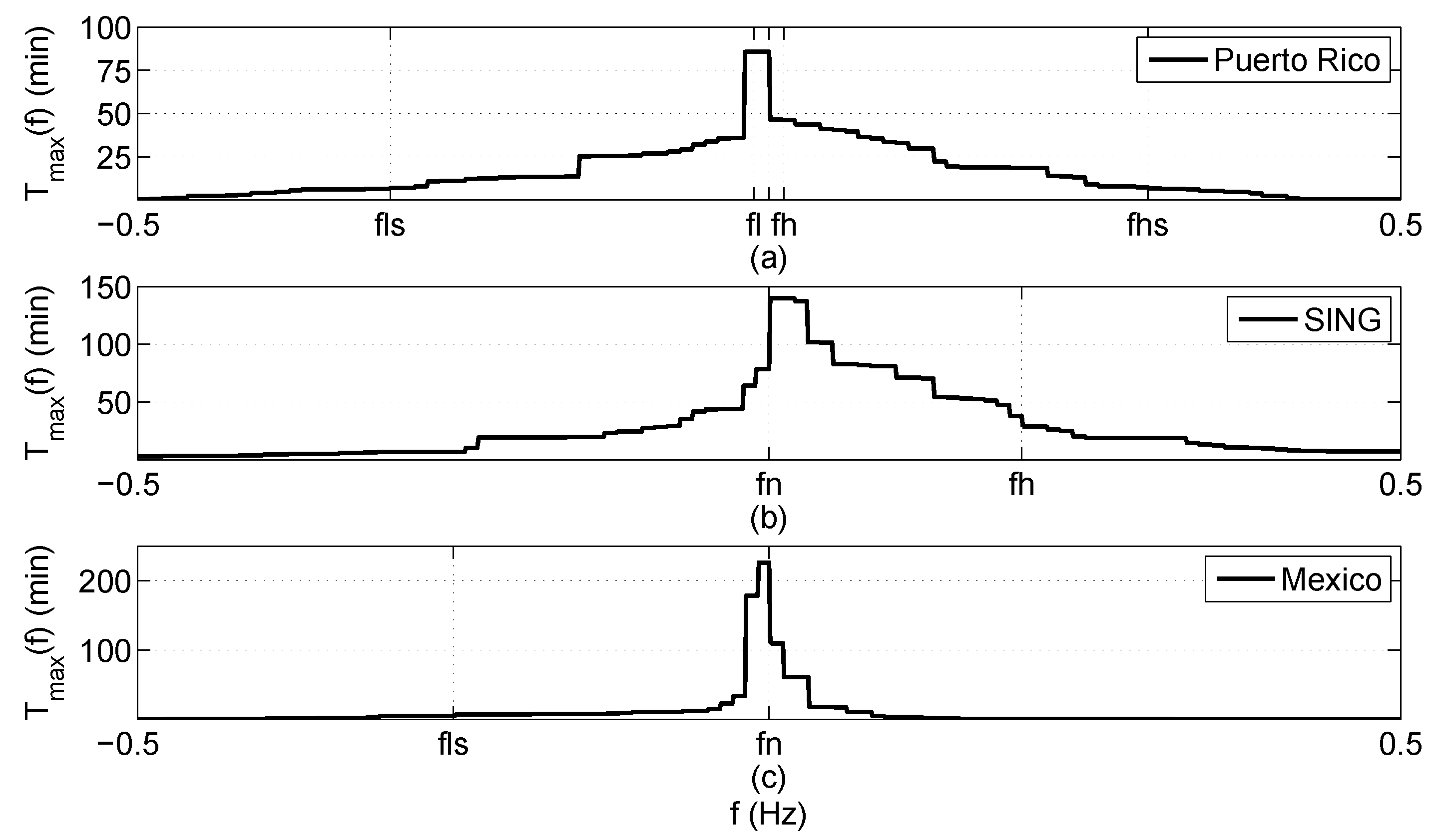
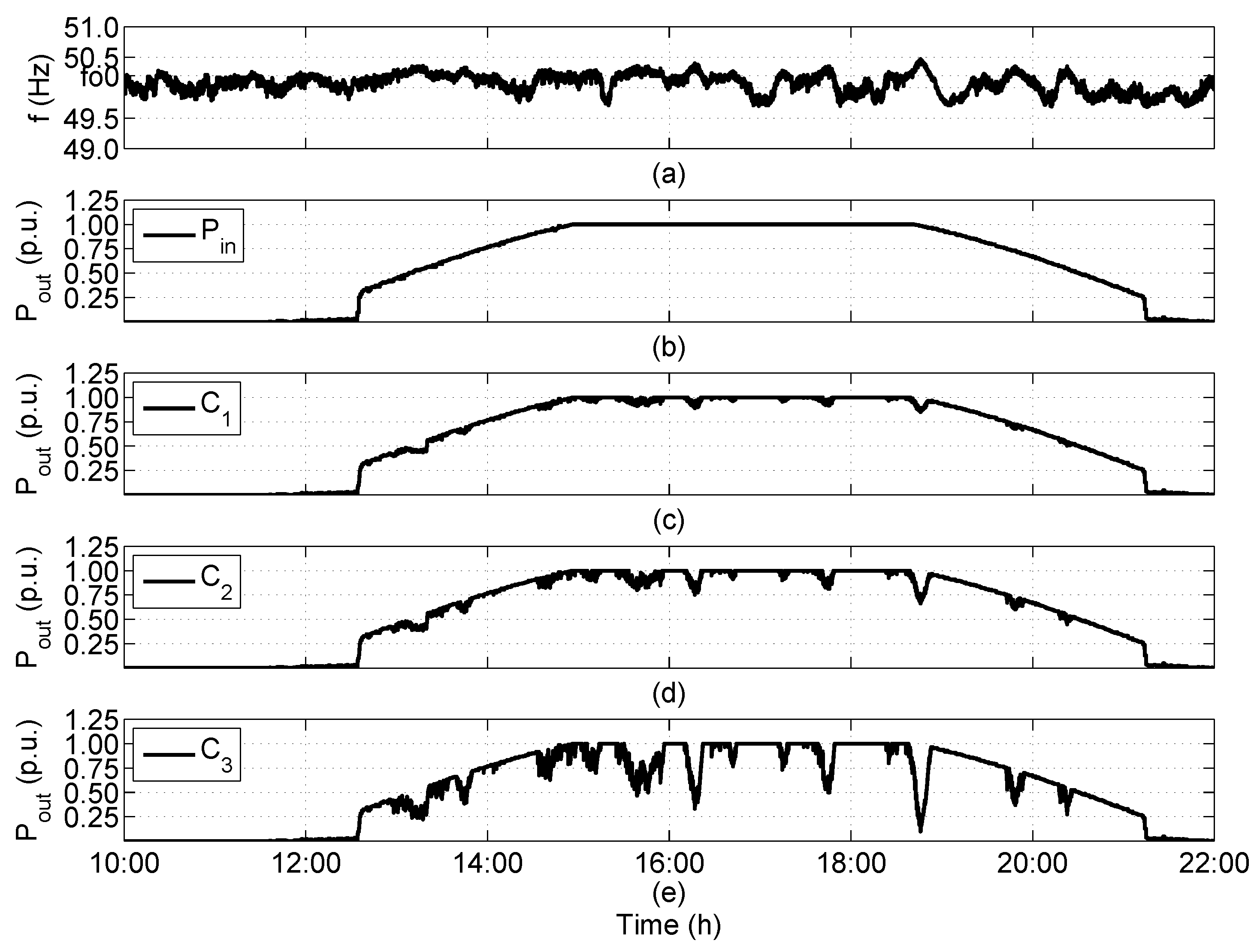
• Frequency excursions could remian for very long inside the range of FR, up to 50 min for some cases.
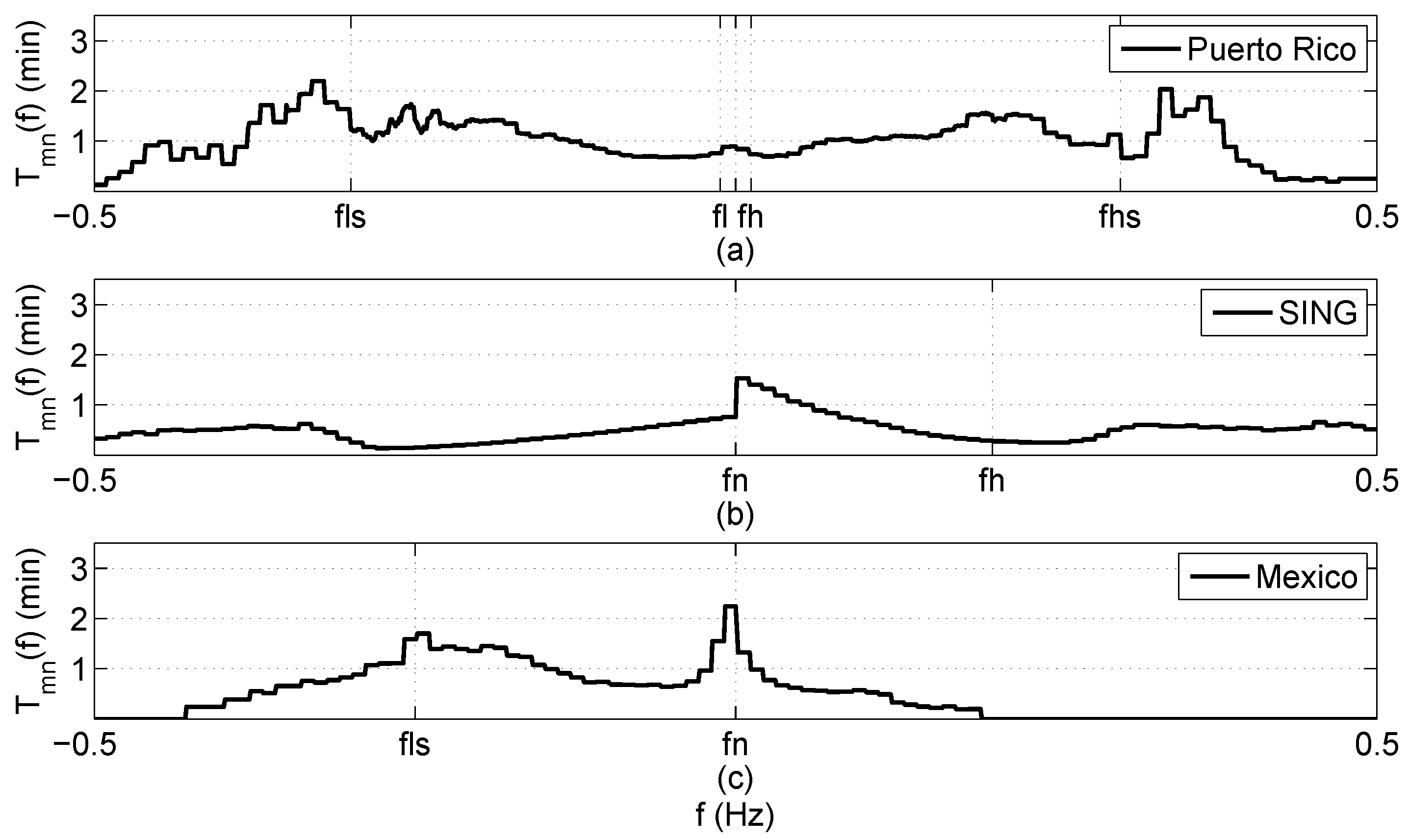
• However, the mean time of frequency excursions is much shorter, about 1 or 2 min for all studied cases.
• When the frequency fault exceeded the FR operating range, the fault duration could be significantly longer. This effect is due to the FR saturation control.
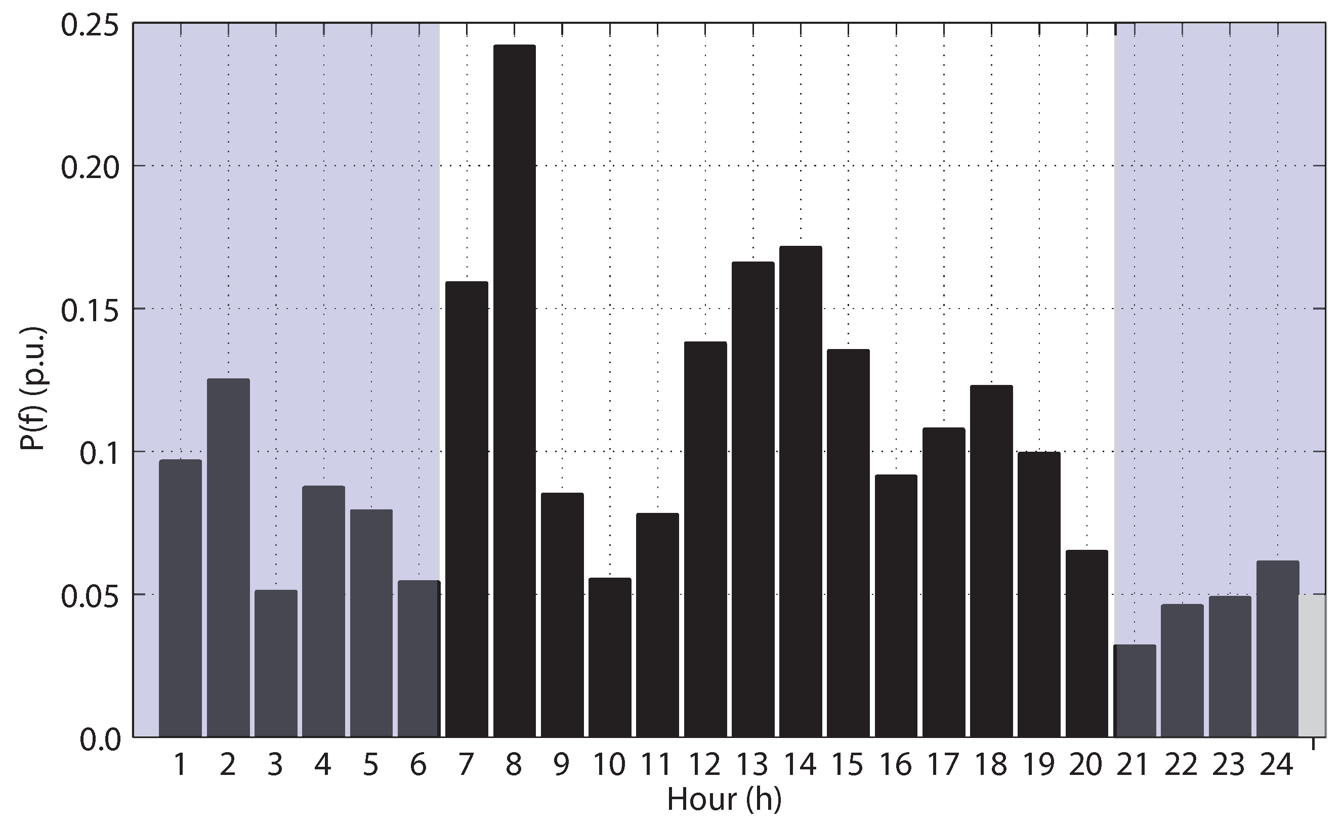
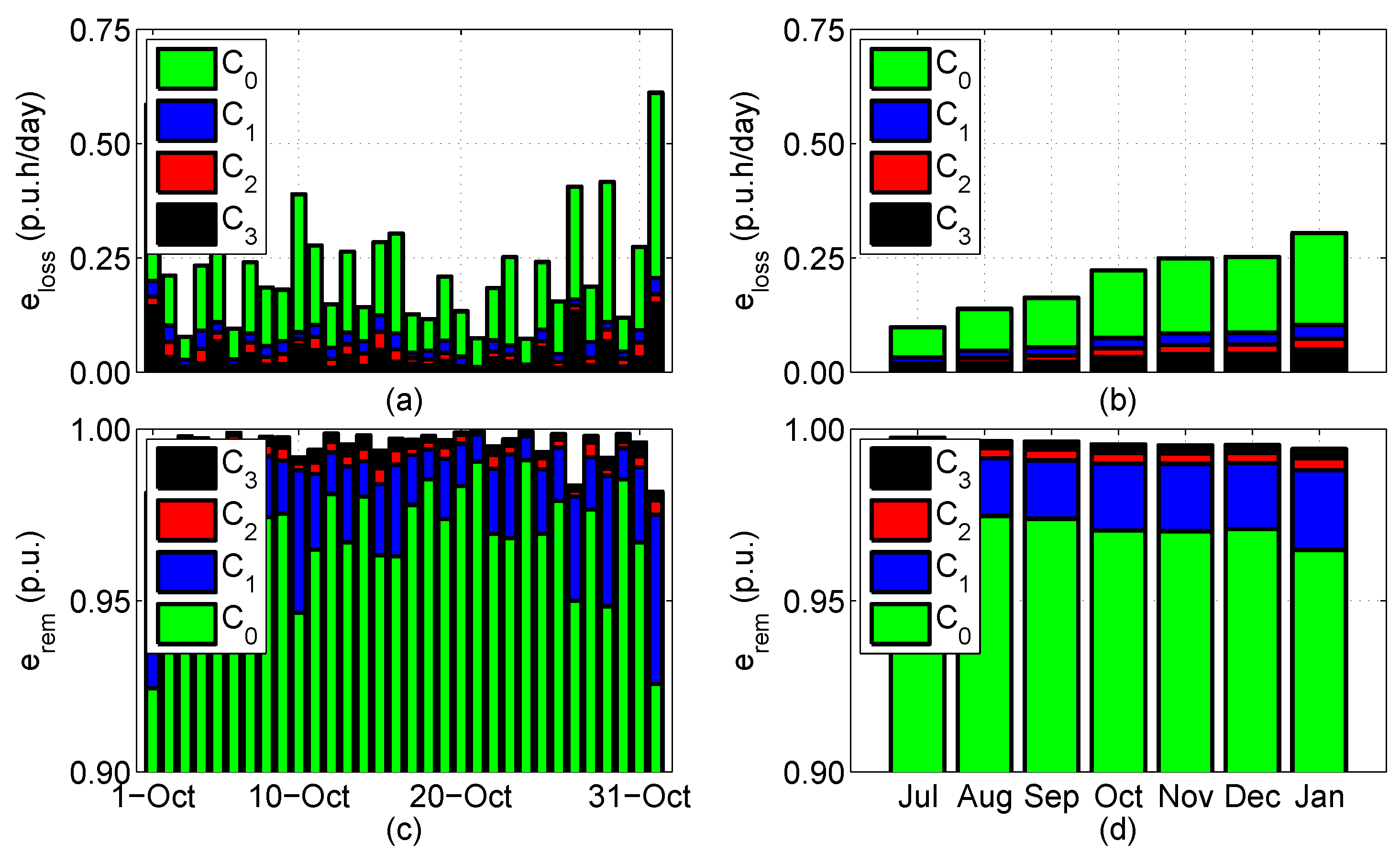
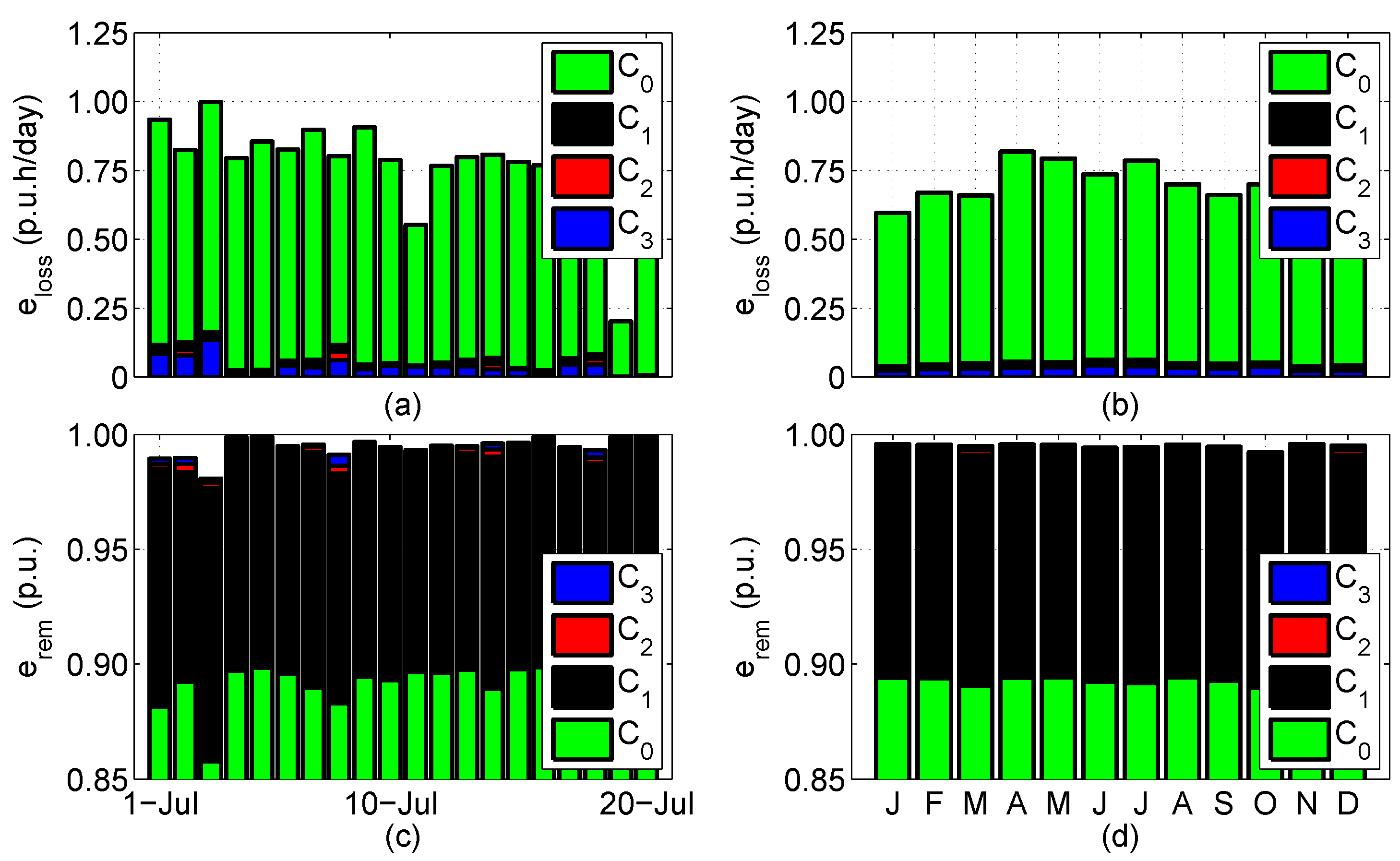
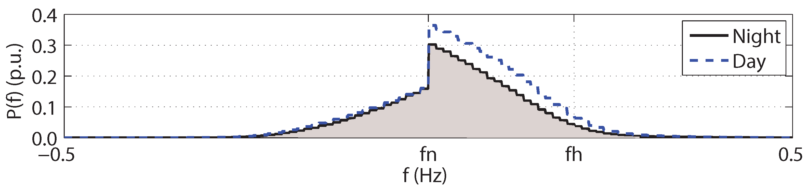
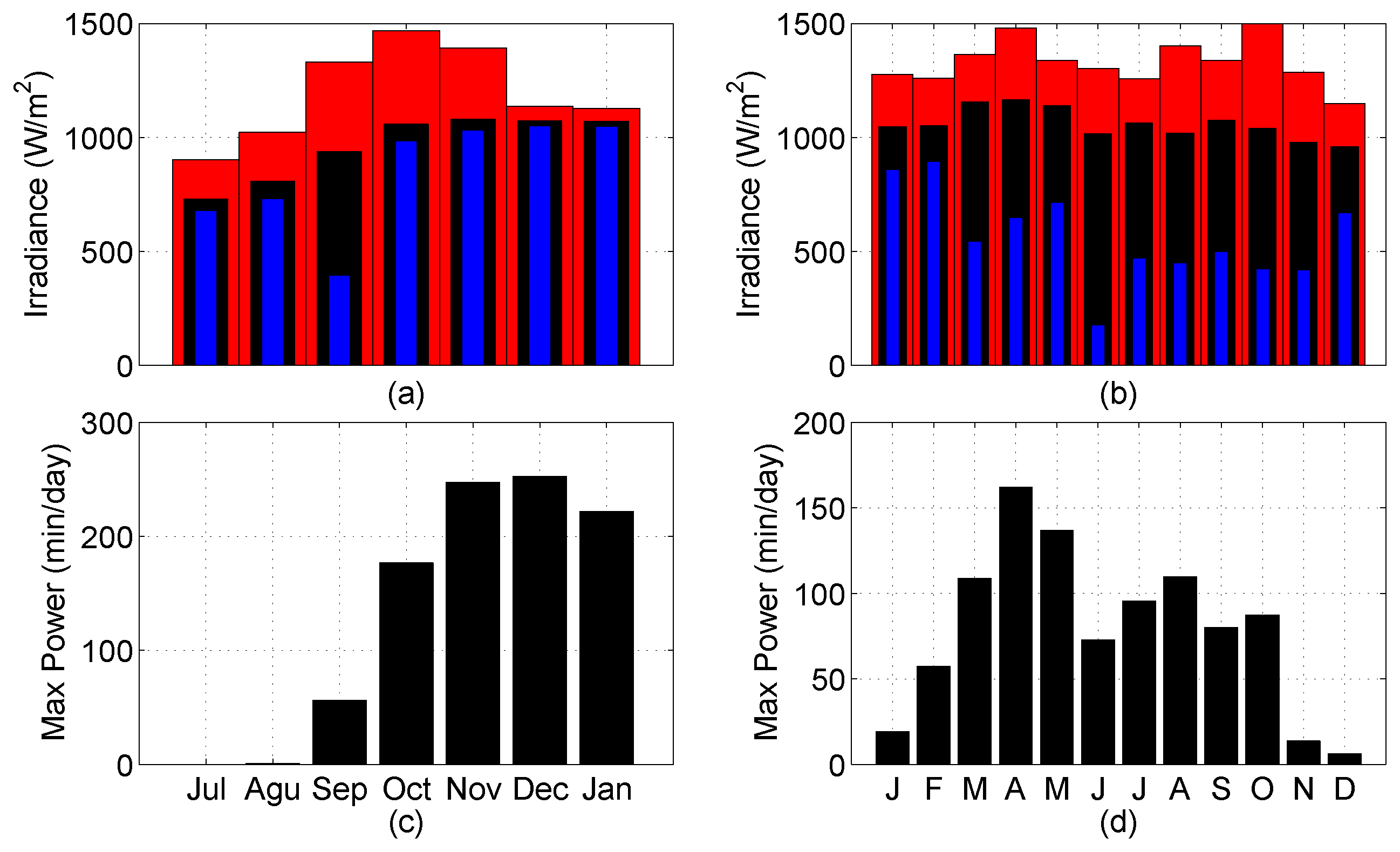
• Frequency excursions are hourly time dependent. The ocurrence probability of faults is higher in day time, increasing USPVP losses. Moreover, it is distributed irregularly with some remarked peaks, probably due to peak demand hours.

PV plants have many advantages: its energy is clean, solar energy is a locally available renewable resource, etc. However, they are more expensive than other alternatives. Worldwide governments encourage solar plants with several types of incentives, in order to maximize the PV plants profits versus other technologies [47,48,49,50,51]. BESS could help to PV plants to become more profitable in some special cases as pointed out above, and contribute to help the grid system stability.

Finally, the introduction of BESS has been proven to help reduce power losses and maximize the efficiency of the power plant, removing PV reserves. The improvement has been quantized with the LCOE estimation, with a reduction up to 1.51 /MWh. This result is very important, because most recent reports point out the necessity of BESS economic incentives due to the high prices of batteries [30,31,32,33].

PV plant owners or utilities could evaluate whether new USPVPs can have economically viable BESS or not. Figure 22 shows a summarised procedure for a correct evaluation. The procedure could be divided into four phases. The first phase collects the most important environmental variables from the new plant’s desired location. Solar irradiance, temperature, location and other input settings build a model to size the USPVP accordingly with the owner’s objectives. The second phase estimates solar production generation ($P_{\text{PV}}$), and a study about the grid frequency stability helps to estimate losses due to FR of national grid code ($P_{\text{FR}}$). After that, the third phase sizes the more convenient BESS system for the studied application, and total power production could be estimated with and without BESS. Finally, the fourth phase calculates investment costs and revenues, and a final decision could be made redarding the most cost-effective solution.

Moreover, introduction of BESS has many other advantages:

• BESS could improve other features as constant power ramp rates over production.
• Energy saved could be used at any time when the utility grid needs it, complementing the uncertainty of renewable sources. Moreover, BESS could perform perform peak shaving actions and load management.
• BESS could be used also as static voltage compensators (SVCs), adding reactive power capacity to the plant.
• BESS could smooth PV plant output production over cloudy conditions.
• BESS could be used to perform load shifting actions to help the grid stability.

References

1. Morjaria, M.; Anichkov, D.; Chadliev, V.; Soni, S. A grid-friendly plant: The role of utility-scale photovoltaic plants in grid stability and reliability. IEEE Power Energy Mag. 2014, 12, 87–95. [Google Scholar] [CrossRef]
2. Grid Connection Code for Renewable Power Plants (RPPs) Connected to the Electricity Transmission System (TS) or the Distribution System (DS) in South Africa; Version 2.6; National Energy Regulator of South Africa (NERSA): Pretoria, South Africa, 2012.
3. Guideline for Generating Plants, Connection to and Parallel Operation with the Medium-Voltage Network; German Association of Energy and Water Industries (BDEW): Berlin, Germany, 2008.
4. Regolazione Tecnica dei Requisiti di Sistema Della Generazione Distribuita; Terna Group: Rome, Italy, 2012. (In Italian)
5. Norma Técnica de Seguridad y Calidad de Servicio; Electric National Commission (CNE): Santiago de Chile, Chile, 2015. (In Spanish)
6. Minimum Technical Requirements for Photovoltaic Generation (PV) Projects; Puerto Rico Electric Power Authority (PREPA): San Juan, Puerto Rico, 2012.
7. Reglas Generales de Interconexión al Sistema Eléctrico; Comisión Federal de Electricidad (CFE): Mexico City, Mexico, 2014. (In Spanish)
8. De Brabandere, K.; Bolsens, B.; Van den Keybus, J.; Woyte, A.; Driesen, J.; Belmans, R. A voltage and frequency droop control method for parallel inverters. IEEE Trans. Power Electron. 2007, 22, 1107–1115. [Google Scholar] [CrossRef]
9. Lu, L.Y.; Chu, C.C. Autonomous Power Management and Load Sharing in Isolated Micro-Grids by Consensus-Based Droop Control of Power Converters. In Proceedings of the Future Energy Electronics Conference, Tainan, Taiwan, 3–6 November 2013; pp. 365–370.
10. Xin, H.; Liu, Y.; Wang, Z.; Gan, D.; Yang, T. A new frequency regulation strategy for photovoltaic systems without energy storage. IEEE Trans. Sustain. Energy 2013, 4, 985–993. [Google Scholar] [CrossRef]
11. Vasconcelos, H.; Moreira, C.; Madureira, A.; Lopes, J.P.; Miranda, V. Advanced control solutions for operating isolated power systems: Examining the Portuguese islands. IEEE Electrific. Mag. 2015, 3, 25–35. [Google Scholar] [CrossRef]
12. Liu, Y.; Xin, H.; Wang, Z.; Gan, D. Control of virtual power plant in microgrids: a coordinated approach based on photovoltaic systems and controllable loads. IET Gener. Transm. Distrib. 2015, 9, 921–928. [Google Scholar] [CrossRef]
13. Trivedi, A.; Jain, D.; Singh, M. A Modified Droop Control Method for Parallel Operation of VSI’s in Microgrid. In Proceedings of the IEEE ISGT Asia, Bangalore, India, 10–13 November 2013; pp. 1–5.
14. Kahrobaeian, A.; Mohamed, Y.R. Robust single-loop direct current control of LCL-filtered converter-based DG units in grid-connected and autonomous microgrid modes. IEEE Trans. Power Electron. 2014, 29, 5605–5619. [Google Scholar] [CrossRef]
15. Rocabert, J.; Luna, A.; Blaabjerg, F.; RodriÌAguez, P. Control of power converters in AC microgrids. IEEE Trans. Power Electron. 2012, 27, 4734–4749. [Google Scholar] [CrossRef]
16. Ashabani, M.; Mohamed, Y.A.R.I. Integrating VSCs to weak grids by nonlinear power damping controller with self-synchronization capability. IEEE Trans. Power Syst. 2014, 29, 805–814. [Google Scholar] [CrossRef]
17. Mahmood, H.; Michaelson, D.; Jiang, J. A power management strategy for PV/battery hybrid systems in islanded microgrids. IEEE Trans. Power Syst. 2014, 2, 870–882. [Google Scholar] [CrossRef]
18. Simpson-Porco, J.W.; Shafiee, Q.; Dorfler, F.; Vasquez, J.C.; Guerrero, J.M.; Bullo, F. Secondary frequency and voltage control of islanded microgrids via distributed averaging. IEEE Trans. Ind. Electron. 2015, 62, 7025–7038. [Google Scholar] [CrossRef]
19. Yuen, C.; Oudalov, A.; Timbus, A. The provision of frequency control reserves from multiple microgrids. IEEE Trans. Ind. Electron. 2011, 58, 173–183. [Google Scholar] [CrossRef]
20. Shi, H.T.; Zhuo, F.; Yi, H.; Wang, F.; Zhang, D.; Geng, Z. A novel real-time voltage and frequency compensation strategy for photovoltaic-based microgrid. IEEE Trans. Ind. Electron. 2015, 62, 3545–3556. [Google Scholar] [CrossRef]
21. Chow, J.H.; Wu, F.F.; Momoh, J.A. Applied Mathematics for Restructured Electric Power Systems; Springer: Berlin/Heidelberg, Germany, 2005. [Google Scholar]
22. Balancing and Frequency Control; North American Electric Reliability Corporation: Princeton, NJ, USA, 2011.
23. Hanley, M.A. Frequency Instability Problems in North American Interconnections; National Energy Technology Laboratory: Pittsburgh, PA, USA, 2011. [Google Scholar]
24. Kouro, S.; Leon, J.I.; Vinnikov, D.; Franquelo, L.G. Grid-connected photovoltaic systems: An overview of recent research and emerging PV converter technology. IEEE Ind. Electron. Mag. 2015, 9, 47–61. [Google Scholar] [CrossRef]
25. Romero-Cadaval, E.; Spagnuolo, G.; Franquelo, L.G.; Ramos-Paja, C.A.; Suntio, T.; Xiao, W.M. Grid-connected photovoltaic generation plants: Components and operation. IEEE Ind. Electron. Mag. 2013, 7, 6–20. [Google Scholar] [CrossRef] [Green Version]
26. Li, X.; Hui, D.; Lai, X. Battery energy storage station (BESS)-based smoothing control of photovoltaic (PV) and wind power generation fluctuations. IEEE Trans. Sustain. Energy 2013, 4, 464–473. [Google Scholar] [CrossRef]
27. Yang, Y.; Li, H.; Aichhorn, A.; Zheng, J.; Greenleaf, M. Sizing strategy of distributed battery storage system with high penetration of photovoltaic for voltage regulation and peak load shaving. IEEE Trans. Smart Grid 2014, 5, 982–991. [Google Scholar] [CrossRef]
28. Abdeltawab, H.H.; Mohamed, Y.A.R.I. Market-oriented energy management of a hybrid wind-battery energy storage system via model predictive control with constraints optimizer. IEEE Trans. Ind. Electron. 2015, 62, 6658–6670. [Google Scholar] [CrossRef]
29. Graditi, G.; Ippolito, M.G.; Telaretti, E.; Zizzo, G. An innovative conversion device to the grid interface of combined RES-based generators and electric storage systems. IEEE Trans. Ind. Electron. 2015, 62, 2540–2550. [Google Scholar] [CrossRef]
30. DiOrio, N.; Dobos, A.; Janzou, S. Economic Analysis Case Studies of Battery Energy Storage with SAM; National Renewable Energy Laboratory: Denver, CO, USA, 2015. [Google Scholar]
31. Battery Storage for Renewables: Market Status and Technology Outlook; International Renewable Energy Agency (IRENA): Abu Dhabi, UAE, 2015.
32. Ekus, B. Storage Incentives or Demand Side Management: Is PV on the Right Track? International Battery & Energy Storage Alliance: Paris, France, 2015. [Google Scholar]
33. Integrated Resource Planning Report; Hawaiian Electric Company: Honolulu, HI, USA, 2013.
34. Gomez-Exposito, A.; Conejo, A.J.; Cañizares, C. Electric Energy Systems: Analysis and Operation; CRC Press: Boca Raton, FL, USA, 2008. [Google Scholar]
35. Roberts, O.; Andreas, A. United States Virgin Islands: St. Thomas (Bovoni) & St. Croix (Longford) (Data); National Renewable Energy Laboratory, CS Division, University of California: Oakland, CA, USA, 1997. [Google Scholar]
36. Solutions for Utility-Scale, Power Management and Grid Integration; GPTech: Seville, Spain, 2015.
37. Sunny Central 800 MV/1000 MV/1250 MV Datasheet; SMA Solar Technology AG: Rocklin, CA, USA, 2015.
38. Ingecon Sun 830TL B300 Indoor Datasheet; Ingetam: Sarrigurem, Spain, 2015.
39. Lave, M.; Ellis, A.; Stein, J.S. Simulating Solar Power Plant Variability: A Review of Current Methods; Sandia National Laboratories: Alburquerque, NM, USA, 2013. [Google Scholar]
40. Lave, M.; Kleissl, J.; Stein, J.S. A wavelet-based variability model (WVM) for solar PV power plants. IEEE Trans. Sustain. Energy 2013, 4, 501–509. [Google Scholar] [CrossRef]
41. Lave, M.; Kleissl, J. Testing a Wavelet-Based Variability Model (WVM) for Solar PV Power Plants. In Proceedings of the IEEE Power and Energy Society General Meeting, San Diego, CA, USA, 22–26 July 2012; pp. 1–6.
42. Lithium Battery Life; La Société des Accumulateurs Fixes et de Traction (SAFT): Bagnolet, France, 2014.
43. Intensium Max 20P High Power Lithium-Ion Container; La Société des Accumulateurs Fixes et de Traction (SAFT): Bagnolet, France, 2013.
44. Advanced Battery for Energy Storage System; Lucky Goldstar Chemicals (LG Chem): Seoul, Korea, 2015.
45. Levelized Cost of Electricity: Renewable Energy Technologies Study; Franhofer ISE: Freiburg, Germany, 2013.
46. Lazard’s Levelized Cost of Electricity Analysis Version 8.0; Lazard: New York, NY, USA, 2014.
47. Sarasa-Maestro, C.; Dulfo-López, R.; Bernal-Agustín, J. Photovoltaic remuneration policies in the European Union. Energy Policy 2013, 55, 317–328. [Google Scholar] [CrossRef]
48. Badcock, J.; Lenzen, M. Subsidies for electricity-generating technologies: A review. Energy Policy 2010, 38, 5038–5047. [Google Scholar] [CrossRef]
49. López Polo, A.; Haas, R. An international overview of promotion policies for grid-connected photovoltaic systems. Prog. Photovolt. Res. Appl. 2014, 22, 248–273. [Google Scholar] [CrossRef]
50. Sgroi, F.; Tudisca, S.; Di Trapani, A.; Testa, R.; Squatrito, R. Efficacy and efficiency of Italian energy policy: The case of PV systems in greenhouse farms. Energies 2014, 7, 3985–4001. [Google Scholar] [CrossRef]
51. Giannini, E.; Moropoulou, A.; Maroulis, Z.; Siouti, G. Penetration of Photovoltaics in Greece. Energies 2015, 8, 6497–6508. [Google Scholar] [CrossRef]
Figure 1. Frequency regulation (FR) classification methods for photovoltaic (PV) applications. AGC: automatic gain controller.
Energies 09 00317 g001
Figure 2. PV converter controller scheme divided into 4 layers: high, middle, low and hardware level. FR method is allocated into the middle layer adjusting the output power reference output.
Energies 09 00317 g002
Figure 3. Converter resident FR scheme, maximum power point tracker (MPPT) output ( P ref ’) is modified by FR algorithm to provide a suitable current output power reference ( P ref ).
Energies 09 00317 g003
Figure 4. Power system resident FR by an AGC. A common control curtailment signal ( P sat curt ) is sent to all inverters.
Energies 09 00317 g004
Figure 5. Battery energy storage system (BESS) control law. BESS power output ( P BESS ) tries to provide the necessary FR active power contribution ( P FR ). If there was not a required FR action, the BESS would recover its initial state of charge ( S O C ini ).
Energies 09 00317 g005
Figure 6. Occurrence probability of a frequency excursion in three different power grids: (a) Puerto Rico (PREPA); (b) Chile (SING); and (c) Mexico (CFE).
Energies 09 00317 g006
Figure 7. Maximum clearing time of frequency excursions in three different power grids: (a) Puerto Rico (PREPA); (b) Chile (SING); and (c) Mexico (CFE).
Energies 09 00317 g007
Figure 8. Mean clearing time of frequency excursions in three different power grids: (a) Puerto Rico (PREPA); (b) Chile (SING); and (c) Mexico (CFE).
Energies 09 00317 g008
Figure 9. Occurrence probability during the day and night of a frequency disturbance in SING power grid.
Energies 09 00317 g009
Figure 10. Hourly frequency disturbance occurrence probability of f h in SING power grid. Shadowed parts point out night time.
Energies 09 00317 g010
Figure 11. Overall irradiance during a year, showing two seasons: Left side shows an example of the irradiance of one day, and the right side the temperature in the same day.
Energies 09 00317 g011
Figure 12. Irradiance measurements statistics over a whole year. Maximum, mean and minimum of maximum daily irradiation in red, black, and blue respectively, for (a) Chile; and (b) Puerto Rico. Expected minutes per day of the plant at full power for (c) Chile; and (d) Puerto Rico.
Energies 09 00317 g012
Figure 13. USPVP active power output ( P out ) and frequency in 15th October in Chile: (a) Registered frequency; (b) Ideal USPVP active power output ( P in ); and (c,d and e) power output applying FR with f 1 = { C 1 , C 2 , C 3 } = { 52 , 51 , 50 . 5 } Hz respectively.
Energies 09 00317 g013
Figure 14. USPVP active power output ( P out ) and frequency in 19th July in Puerto Rico: (a) Registered frequency; (b) Ideal USPVP active power output ( P in ); and (c) power output applying FR ( C 1 ).
Energies 09 00317 g014
Figure 15. USPVP energy losses due to FR during a year in Chile, with f 1 at 52, 51 and 50.5 Hz, ( C 1 , C 2 and C 3 respectively): (a) Daily energy losses ( e loss ) in October; (b) monthly energy losses; (c) daily remnant energy ( e rem ) in October; and (d) monthly remnant energy.
Energies 09 00317 g015
Figure 16. USPVP energy losses due to FR during a year in Puerto Rico: (a) Daily energy losses ( e loss ) in July; (b) monthly energy losses; (c) daily remnant energy ( e rem ) in July; and (d) monthly remnant energy.
Energies 09 00317 g016
Figure 17. Number of cycles (NOC) v s . depth of discharge (DOD) of the selected BESS.
Energies 09 00317 g017
Figure 18. USPVP energy losses due to FR during a year in Chile, with f 1 at 52 Hz, for several ESS scenarios: C at 0.00277 p.u.h ( C 1 ), 0.00833 p.u.h ( C 2 ), 0.015 p.u.h ( C 3 ) and without BESS ( C 0 ): (a) Daily energy losses ( e loss ) in October; (b) monthly energy losses; (c) daily remnant energy ( e rem ) in October; and (d) monthly remnant energy.
Energies 09 00317 g018
Figure 19. USPVP energy losses due to FR during a year in Puerto Rico, for several ESS scenarios: C at 0.00277 p.u.h ( C 1 ), 0.00833 p.u.h ( C 2 ), 0.015 p.u.h ( C 3 ) and without BESS ( C 0 ): (a) Daily energy losses ( e loss ) in July; (b) monthly energy losses; (c) daily remnant energy ( e rem ) in July; and (d) monthly remnant energy.
Energies 09 00317 g019
Figure 20. BESS sizing results for SING case considering a whole year of transient results data, values of f 1 at 52, 51 and 50.5 Hz, C 1 , C 2 and C 3 respectively: (a) Daily energy losses ( e loss ) per BESS capacity; and (b) end of life (EOL) per BESS capacity.
Energies 09 00317 g020
Figure 21. BESS sizing results for Puerto Rican case considering a whole year of transient results data: (a) Daily energy losses per BESS capacity; and (b) EOL per BESS capacity.
Energies 09 00317 g021
Figure 22. Summarised procedure to evaluate BESS whether new USPVPs can have economically viable BESS or not. Four phases are clearly distinguished: Phase 1: USPVP sizing; Phase 2: solar production generation and FR losses estimation; Phase 3: BESS sizing and total power production estimation; and Phase 4: LCOE calculation and decision.
Energies 09 00317 g022