
One-Dimensional Modelling of Marine Current Turbine Runaway Behaviour

Division of Electricity, Department of Engineering Sciences, Uppsala University, P.O. Box 534, SE-751 21 Uppsala, Sweden
*
Author to whom correspondence should be addressed.
Energies 2016, 9(5), 309; https://doi.org/10.3390/en9050309
Submission received: 12 February 2016
/
Revised: 6 April 2016
/
Accepted: 13 April 2016
/
Published: 25 April 2016
(This article belongs to the Special Issue Numerical Modelling of Wave and Tidal Energy)
Abstract
:If a turbine loses its electrical load, it will rotate freely and increase speed, eventually achieving that rotational speed which produces zero net torque. This is known as a runaway situation. Unlike many other types of turbine, a marine current turbine will typically overshoot the final runaway speed before slowing down and settling at the runaway speed. Since the hydrodynamic forces acting on the turbine are dependent on rotational speed and acceleration, turbine behaviour during runaway becomes important for load analyses during turbine design. In this article, we consider analytical and numerical models of marine current turbine runaway behaviour in one dimension. The analytical model is found not to capture the overshoot phenomenon, while still providing useful estimates of acceleration at the onset of runaway. The numerical model incorporates turbine wake build-up and predicts a rotational speed overshoot. The predictions of the models are compared against measurements of runaway of a marine current turbine. The models are also used to recreate previously-published results for a tidal turbine and applied to a wind turbine. It is found that both models provide reasonable estimates of maximum accelerations. The numerical model is found to capture the speed overshoot well.
1. Introduction
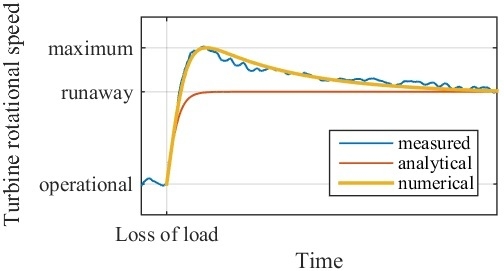
If during the operation of a marine current turbine the electrical load is lost for any reason, the turbine will rotate freely and increase speed, eventually settling at the rotational speed that produces zero net torque. This is known as the runaway or no-load speed. The turbine will typically overshoot the runaway speed considerably, since the turbine captures more power from the water flow before a wake has developed downstream. The hydrodynamic forces to which the turbine blades are subjected are dependent on rotational speed and acceleration. It follows that rotational runaway speed overshoot becomes an important consideration in fault handling for these turbines.
Runaway speed overshoot has been observed in simulations and scale model tests of horizontal axis tidal turbines [1]. In wind turbines, whose greater inertia in comparison to that of the medium in which they operate makes for a slower and less dynamic increase in rotational speed [2], the phenomenon of overshoot is not nearly as noticeable. Neither does overshoot of the no-load speed seem to be an issue in the case of a runaway hydropower turbine [3]. For a marine current turbine, however, the limiting case in terms of speeds and forces to which the turbine may be subjected will be that of maximum runaway speed overshoot rather than the no-load speed itself.
In this article, we consider analytical and numerical models of marine current turbine runaway behaviour in one dimension. The analytical model is found not to capture the overshoot phenomenon, while still providing useful estimates of acceleration at the onset of runaway. The numerical model incorporates turbine wake build-up and predicts a rotational speed overshoot. The predictions of the models are compared against measurements of turbine runaway.
2. Modelling
Consider a turbine runner with fixed-pitch blades, directly connected by a shaft to the rotor of a generator. The rotational energy of the turbine is:
where J is the mass moment of inertia of the rotating system (turbine runner, shaft and generator rotor) and is the angular velocity at which the turbine is operating. The time derivative of E is the power P:
However, power is also torque Q times angular velocity, so we get:
The torque has a hydrodynamic component, a load component and a component due to mechanical and electrical losses:
According to momentum theory (see, for instance, Chapter 3 in [4]), the hydrodynamic driving torque is proportional to the flow speed u and the angular velocity. Hydrodynamic drag causes a torque loss proportional to the angular velocity squared. We get:
where k and k are constants.
The load torque contribution is due to an electrical load being connected to the generator. It is calculated as power dissipated in the load (including cabling) and in the generator (copper losses, where eddy current losses are neglected, since they can be expected to be small [5]) divided by the angular velocity:
Here, the minus sign indicates that the load torque is negative in the sense that it causes power to leave the rotating system.
The torque loss component is caused by friction in bearings and seals and by iron losses in the generator. The frictional torque is constant. The iron losses in turn have several contributing components, such as eddy currents and hysteresis effects in the stator [5]. Iron losses occur regardless of whether any electrical load is connected or not. Due to the low rotational speeds typical of direct-driven generators, power losses other than those proportional to the electrical frequency (which in turn is proportional to the angular velocity of the rotor) are neglected. Consequently, the torque contribution due to iron losses is constant. The torque loss then can be written:
Altogether, we get:
which is the governing equation for turbine rotational speed when a load is connected. If the electrical load is disconnected, the load torque term disappears, and Equation (8) becomes:
This is the governing equation during runaway.
2.1. Analytical Model
To derive an analytical expression for the development of over time during runaway, we assume that the flow speed u seen by the turbine is constant. Then, Equation (9) is a separable first-order nonlinear ordinary differential equation with the solution:
where C is a constant of integration. If the initial condition is applied that operational angular velocity is at time , we get:
The constants k, k and k as well as the inertia of the rotating system J are determined by properties of the actual turbine being modeled. Of these, J and k have to be measured (or calculated) directly. k and k can be determined from the governing equation. Suppose that the turbine operates in a flow with freestream speed u and that the electric power P delivered at an operational angular velocity is known, as well as the runaway angular velocity in the same flow speed. When the turbine runs at constant rotational speed, the left-hand sides of Equations (8) and (9) are 0, and we get:
and:
Solving for k, Equation (13) yields:
which, when substituted into Equation (12), gives:
which in turn can be solved for k, yielding:
Since , the constants are all positive. Typically, the numerical value of k will be at least an order of magnitude lower than that of the other two. Consequently, the expression under the root sign in Equation (10) will be negative and the argument of the arctan function in the expression for C imaginary. C will be complex in general, but its real part will be either 0 or , and the second term of the tan argument in Equation (10) will be purely imaginary, so the value of the tan function will also be purely imaginary. In all, the expression for will be real-valued.
Figure 1 shows a schematic example of the development of angular velocity as predicted by Equation (10). Examining the equation further, we see that:
which, when , simplifies to:
as expected. Looking at the time derivative:
we see that apart from very low flow speeds and rotational speeds, when the driving torque will not overcome the mechanical losses, is monotonously increasing towards if and decreasing if . We have to conclude that the analytical model will not capture the runaway overshoot phenomenon, but it may still prove useful in estimating accelerations.
2.2. Numerical Model
Consider the flow speed u. The mechanism behind the runaway speed overshoot is the fact that the apparent flow speed u seen by the turbine is not constant, but dependent on rotational speed . Furthermore, there is a time lag before the flow speed adapts to a new rotational speed of the turbine. Like the flow speed in the wake, the apparent speed is lower than the freestream speed u, although not as low as the wake speed. If the rotational speed of the turbine is kept constant, the wake will develop and the apparent speed will settle at some steady speed u, which is a function of the freestream speed and the angular velocity of the turbine.
According to momentum theory [4], the flow speed at the turbine in steady-state operation can be determined from the speed in the far wake. The flow speed deficit at the turbine is half the deficit in the downstream wake. Differently put, this means the speed at the turbine is the mean of the free stream speed and the wake speed:
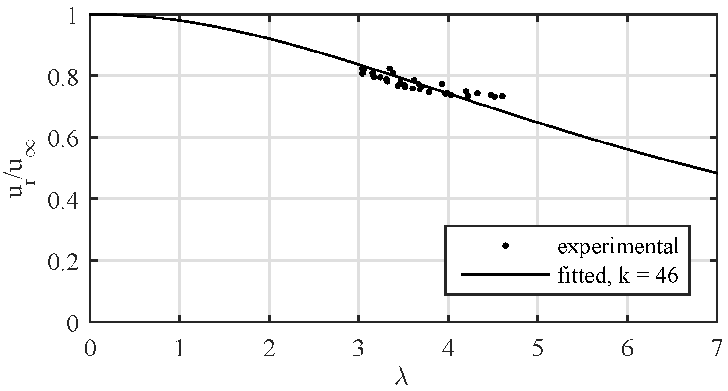
where u is the flow speed at the turbine runner and u is the speed in the wake downstream. Measurements made of the wake downstream of a turbine (Section 3.4) suggest that the normalized turbine flow speed as a function of tip speed ratio can be approximated as:
where k is a constant. is defined as:
where R is the turbine radius. For our model, we assume that u can be taken as u, which is then:
where the constant k will have to be experimentally determined.
Thus, we have:
This means the constants k and k will depend on u. If the (steady) apparent flow speed associated with the operational angular velocity is u and that associated with is u, we get the following expressions for k and k in the same manner as we derived Equations (14) and (16):
and:
Now, our model has to handle the temporal development of both the rotational speed of the turbine and the apparent flow speed in which the turbine operates. In order to do this, we consider the rotational energy of the turbine and the kinetic energy of the flow and how these quantities vary with time.
Suppose the turbine operates in a volume V of water of size:
where is the turbine diameter, is the projected turbine cross-sectional area in the direction of flow, and k is a constant giving the length of the volume in turbine diameters. In this volume, the flow speed is assumed to be, in some average sense, u. Then, the kinetic energy in this volume is:
During steady operation, when the wake is fully developed and , is constant, and we can solve Equation (8) for to get:
This is the net power delivered by the turbine in steady operation, so we change the subscript to “steady”. Since , we can write as a function of the tip speed ratio:
The momentaneous power P delivered by the turbine is:
Due to the inertial properties of the turbine and of the flow, u will not always be equal to u. If the electrical load or the freestream flow speed is changed, and u will in time adapt to the new premises.
During runaway, there is no electrical load connected to which the turbine can deliver captured power. Instead, the rotational energy and, thus, the rotational speed of the turbine will change. If , will increase. For high rotational speeds, however, hydrodynamic drag and mechanical losses will slow the turbine down. Decreasing means . For our model, we will conjecture that the turbine always captures P from the freestream flow, but that the balance , whether more or less than 0, comes from the operational volume V. This way, u will tend towards u in time.
3. Measurements
3.1. The Söderfors Test Site
Experiments were carried out at the Söderfors experimental station operated by Uppsala University (Uppsala, Sweden). A vertical axis turbine is located in a river downstream of a conventional hydro power plant. The turbine axis is directly connected to a permanent magnet synchronous generator. Acoustic Doppler current profilers (ADCP) are mounted upstream and downstream of the turbine. A measurement and control station is on shore. Details of the experimental station can be found in [6,7]. Relevant characteristics are listed in Table 1.
3.2. Performance of Measurements
The turbine was made to run at some rotational speed, governed by the water speed and the electrical load. The load was then removed instantly, and the turbine was allowed to accelerate freely. The line-to-line voltages and phase currents of the generator were measured at a rate of 2000 Hz. From these measurements, the electrical frequency of the generator was deduced, and from this frequency, the angular velocity was calculated. When a load was connected, electrical power delivered by the turbine could also be determined.
The electrical frequency was calculated by identifying consecutive zero-crossings of the line-to-line voltage on one phase. The time from one zero-crossing from negative to positive voltage to the next zero-crossing in the same direction is the time of one electrical period. The mean electrical frequency f during that period is:
and this frequency was associated with the point in time midway between the two zero-crossings. In this manner, a time-history of the electrical frequency was obtained.
Since the generator has 112 poles, there are 56 electrical periods to one revolution of the rotor and turbine. There are radians to a period. Thus, the angular velocity of the turbine is obtained as:
Water speed was monitored using ADCP located approximately two turbine diameters upstream and downstream of the turbine. Each ADCP would measure a vertical profile of the water velocity with 0.25 m between measurement bins once every 3.6 s. A cubic mean velocity magnitude was then computed over those measurement bins covering the turbine.
3.3. Turbine Reference Measurements
In order to determine the constants k and k, the turbine was connected to a symmetric three-phase resistive load of 2.24 Ω per phase plus the resistance in the cables, 0.252 Ω per phase. With this load and flow speed, the turbine operated at roughly nominal operational speed. The turbine was started and allowed to run for several minutes in order for the wake to develop. The mean electrical power (including copper losses in the generator windings) and angular velocity over the next 30 min were calculated. The load was disconnected, and the mean runaway speed was similarly measured over a 30-min period. For results, see Table 2.
3.4. Wake Speed
Measurements of the mean wake speed were taken by the downstream ADCP under various conditions. The rotational speed of the turbine operating under different loads was recorded. Mean values over 30-min runs were computed. Furthermore, the undisturbed water speed (with still standing turbine) was recorded.
3.5. Runaway
Rotational speed was measured during runaway from four different initial conditions:
- (a)
- Nominal rotational speed, i.e., load disconnect during operation at or near the optimum power coefficient C. This was assumed to be the most likely scenario, a fault occurring during normal operation of the turbine.
- (b)
- Zero rotational speed, where the turbine was allowed to self-start. This was taken as the worst possible scenario, since when starting from 0, there is no wake at all behind the turbine, and the runaway speed overshoot is likely to be the highest under these circumstances.
- (c)
- Rotational speed below nominal speed, but not 0. This would be a not unlikely operational scenario in case of unusually high water speeds, when it could be desirable to operate at lower than peak C.
- (d)
- Rotational speed above nominal speed, but not runaway speed. While not a highly likely operational case, it was deemed useful for completeness.
A total of 53 runs were made in the four categories. Results are discussed in Section 4.2.
4. Implementation and Evaluation
The analytical and the numerical model were both implemented using MATLAB. For the numerical model, a fourth order Runge–Kutta scheme was used in time.
4.1. Calibration
For implementation of the analytical model, the constants k through k plus the radius R and inertia J of the turbine need to be determined. For the numerical model, constants k and k are also required.
For the Söderfors turbine, R, k and J are known quantities (Table 1). Together with the reference measurements tabulated in Table 2, this is sufficient to establish k and k for the analytical model by way of Equations (14) and (16).
For the numerical model, k and k according to Equations (25) and (26) depend on for the operational and runaway rotational speeds. u is given by Equation (23) and depends on k, and how quickly u changes depends on the size of V and consequently on k. k was determined by curve fitting as described in Section 3.4.
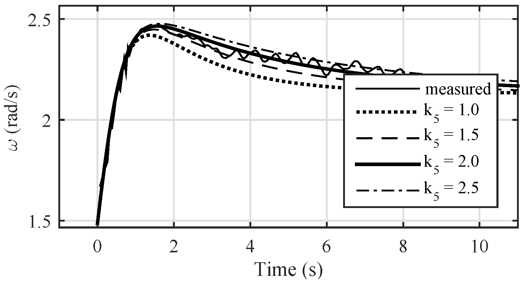
k is in a sense a measure of the size of V, but it cannot be directly measured. To determine a reasonable value of this constant, a large number of runs were made with the numerical model varying this parameter and compared to the measurements of runaway from nominal speed. A few examples are plotted in Figure 3. For simplicity, k was taken as .
4.2. Comparison with Measured Data
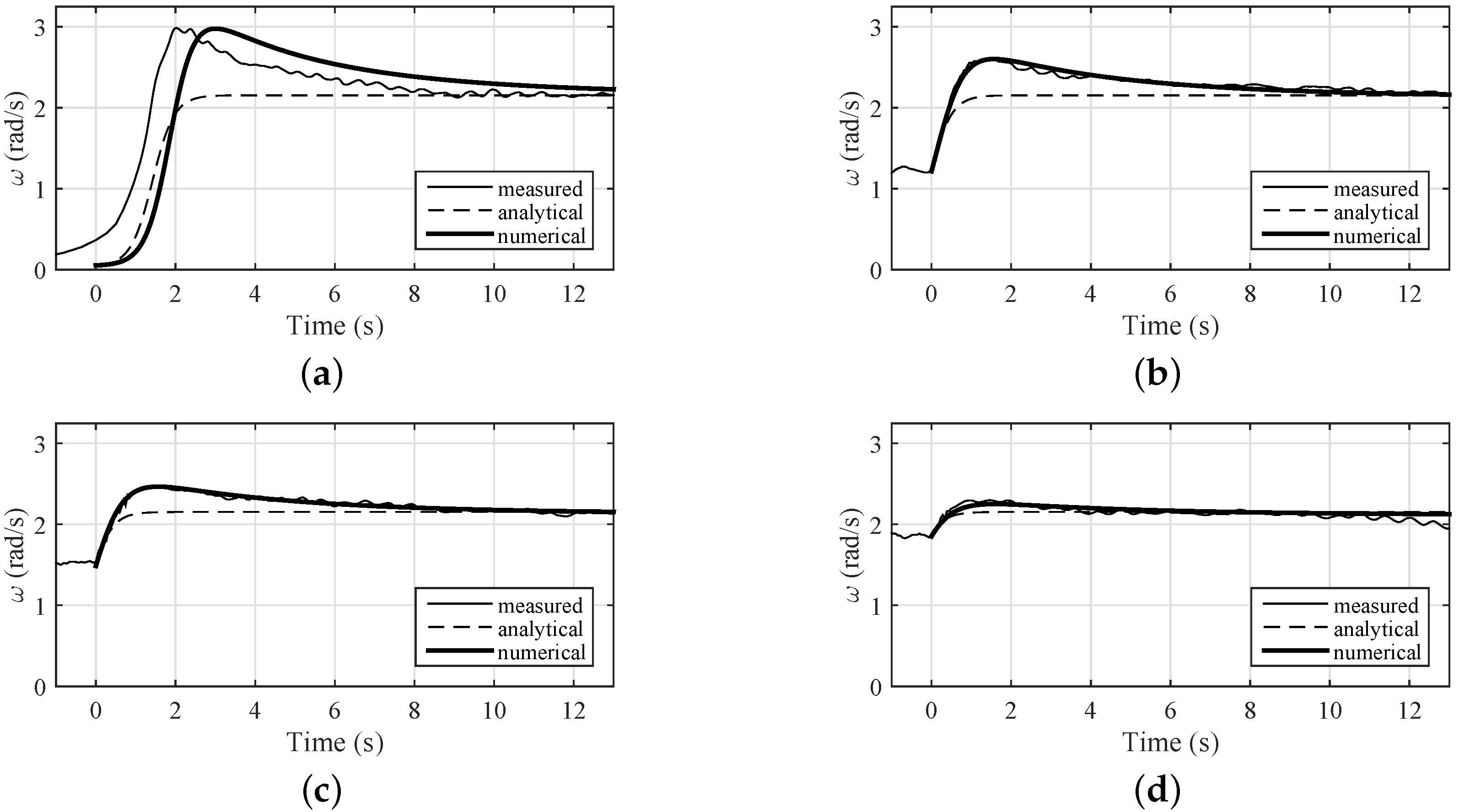
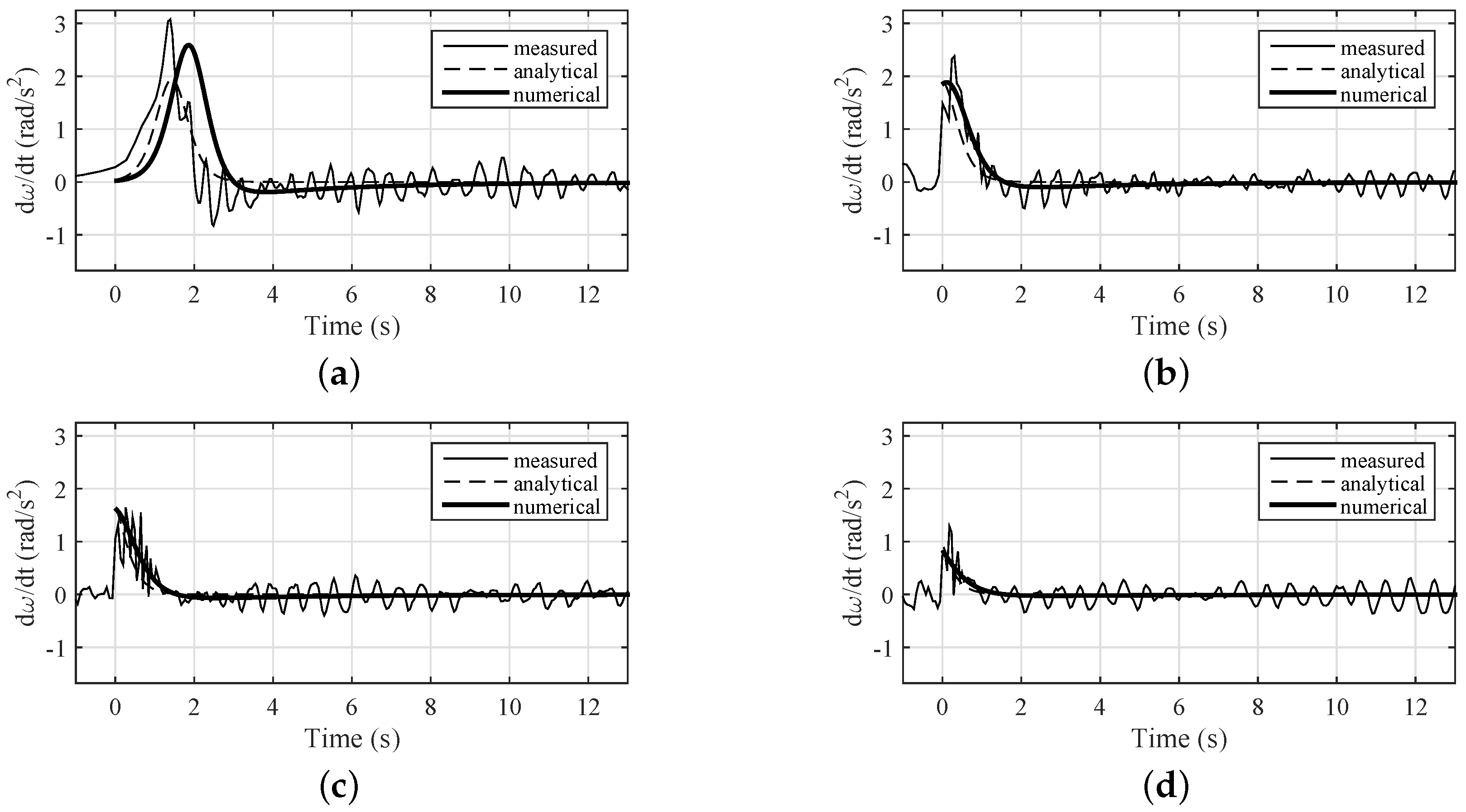
The predictions of the two models were compared to the measurements outlined in Section 3.5. Examples are shown in Table 3 and Figure 4 and Figure 5.
The analytical model does not predict the overshoot, as expected. Initially, it does compare well to the numerical model and the measured results in terms of acceleration. The increase in rotational speed is in reasonable agreement with the measured values for the first few moments, until the analytical model starts to get close to the runaway speed, which it will not exceed.
The numerical model agrees very well with the measured results in terms of peak rotational speed and acceleration.
For the case when the turbine is released from stand-still, there is a significant time lag between the measured results, on the one hand, and those simulated, on the other. This is due to the fact that for very low rotational speeds, the turbine does not behave exactly as the derivation of the models presumes. The starting torque of the turbine is dependent on the exact location of the turbine blades in relation to the direction of flow, while the numerical model assumes that hydrodynamic torque is independent of blade position. Since a vertical axis turbine is not self-starting in theory, the models had to be set off at a non-zero (albeit small) initial angular velocity. For the experimental measurements, rotational speed is deduced from electrical frequency (Section 3.2). By this method, it is not entirely clear at exactly which point the turbine starts to move, i.e., what point in time to pick as . In all, it is difficult to synchronize the numerical results with the measurements.
Both models are dependent on the freestream water speed u. The constants k and k are calculated from a reference run at some u, but if the free stream speed changes, this will affect other runs. The value for u applied in each case is listed in Table 3. It can be noted that the measured rotational speed drops off towards the end of run . This is probably due to a decrease in u, which the model is not capable of emulating.
Figure 5 shows second-order numerical derivatives of the curves in Figure 4. The ‘ripple’ seen in the measured rotational speeds, due to the individual blades of the turbine, is enhanced in the derivative. Having said that, the numerical model catches the general temporal development of the accelerations reasonably well.
Initial numerical and analytical accelerations agree well in magnitude for all cases, except when the turbine is released from standstill. The initial acceleration is also the highest in these cases. This indicates an estimate of the maximum loading on the turbine blades due to acceleration might be obtained from the analytical model.
Figure 6 shows initial and maximum accelerations predicted by the two models plotted with initial accelerations for a large number of experiments. As can be seen, for cases where is close to or larger than , maximum acceleration occurs at the very onset of runaway. In this region, the analytical and numerical models furthermore agree very well on the magnitude of that acceleration, and the experimental values are as a rule smaller than the maximum values predicted by the numerical model. For experimental runs starting at , it was difficult to identify the exact starting point of runaway where to calculate the initial acceleration (see reasoning above), and so, no experimental values of initial acceleration are plotted for those runs.
Figure 7 shows the overshoot, or maximum angular velocity during runaway, predicted by the numerical model as a function of the initial angular velocity and the corresponding experimental values. The numerical model appears to capture the general trend remarkably well.
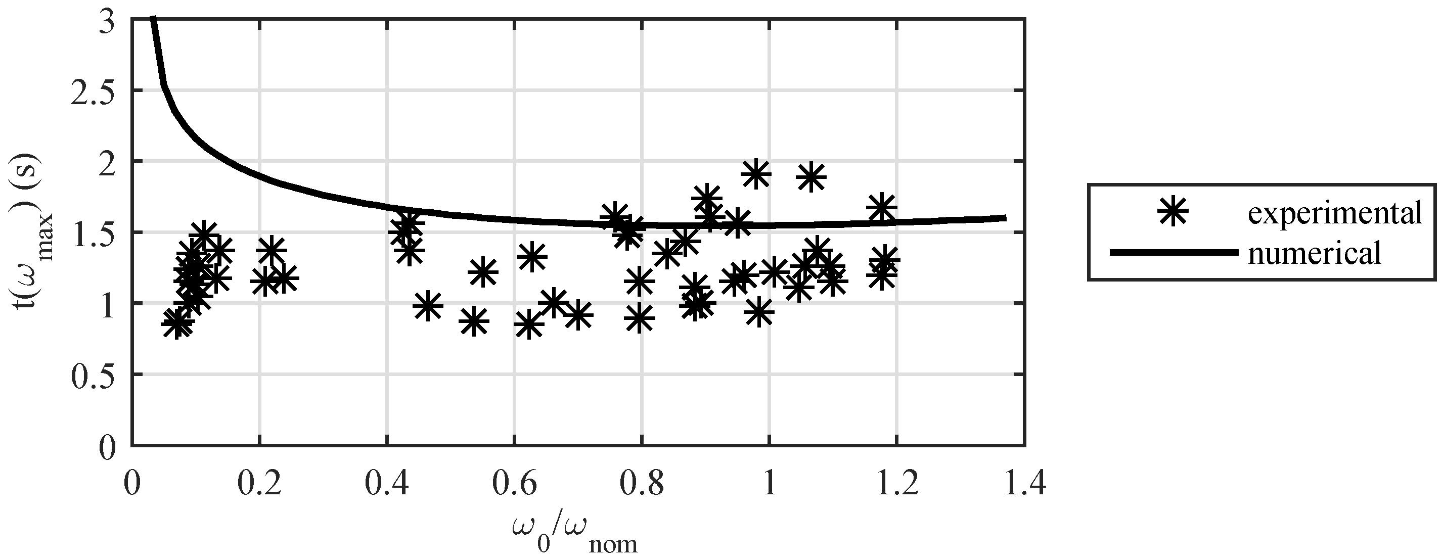
The time in seconds after release at which maximum speed occurs is plotted in Figure 8. The numerical model tends to overestimate the time taken to reach peak angular velocity. When runaway occurs from low initial speeds, due to the difficulty in identifying a starting point on the experimental runs, on the order of half a second should probably be added to the experimental values. These observations are consistent with the examples shown in Figure 4.
4.3. Comparison with Published Results
As mentioned in the Introduction, not a whole lot of work has been published on the subject of runaway speed overshoot. One example is [1], where a scale model experiment on a horizontal axis turbine was reported where overshoot was observed. The paper includes derivation of an analytical model based on the assumption of a linear relationship between angular velocity and torque.
Based on details of the turbine reported in the paper, it was possible to estimate values of k and k. k was assumed to be negligible. For turbine inertia, the analytical results reported seem to indicate 12.4 kg·m. Together with the values for k and k used for the Söderfors turbine, no useful results were obtained. The work in [1] mentions an estimated added inertia of 10% at the onset of runaway, noting that it may be different at other points in the process. Even with this small increase in inertia, good results were not achievable. However, with J = 18 kg·m, = 6 and = 1, the plot in Figure 9 was obtained. The numerical curve agrees well with the measured results presented in Figure 6 of [1], particularly in terms of initial acceleration and magnitude and timing of maximum runaway speed overshoot. The analytical model of [1] gives a higher initial acceleration than our model, due to the considerably lower moment of inertia. The driving torque, however, decreases more quickly than in our model due to the assumed linearity and, consequently, so does acceleration. Both analytical models still reach the runaway speed approximately simultaneously.
4.4. Application to Wind Power Turbine
For comparison, the model was applied to a vertical axis wind turbine. No measurements of runaway behaviour for this turbine was available. The constants k and k for the Söderfors marine current turbine were applied. Since these constants are associated with wake properties, which in turn are to a degree a function of turbine type (vertical or horizontal axis), they were assumed to be a reasonable estimate for the wind turbine.
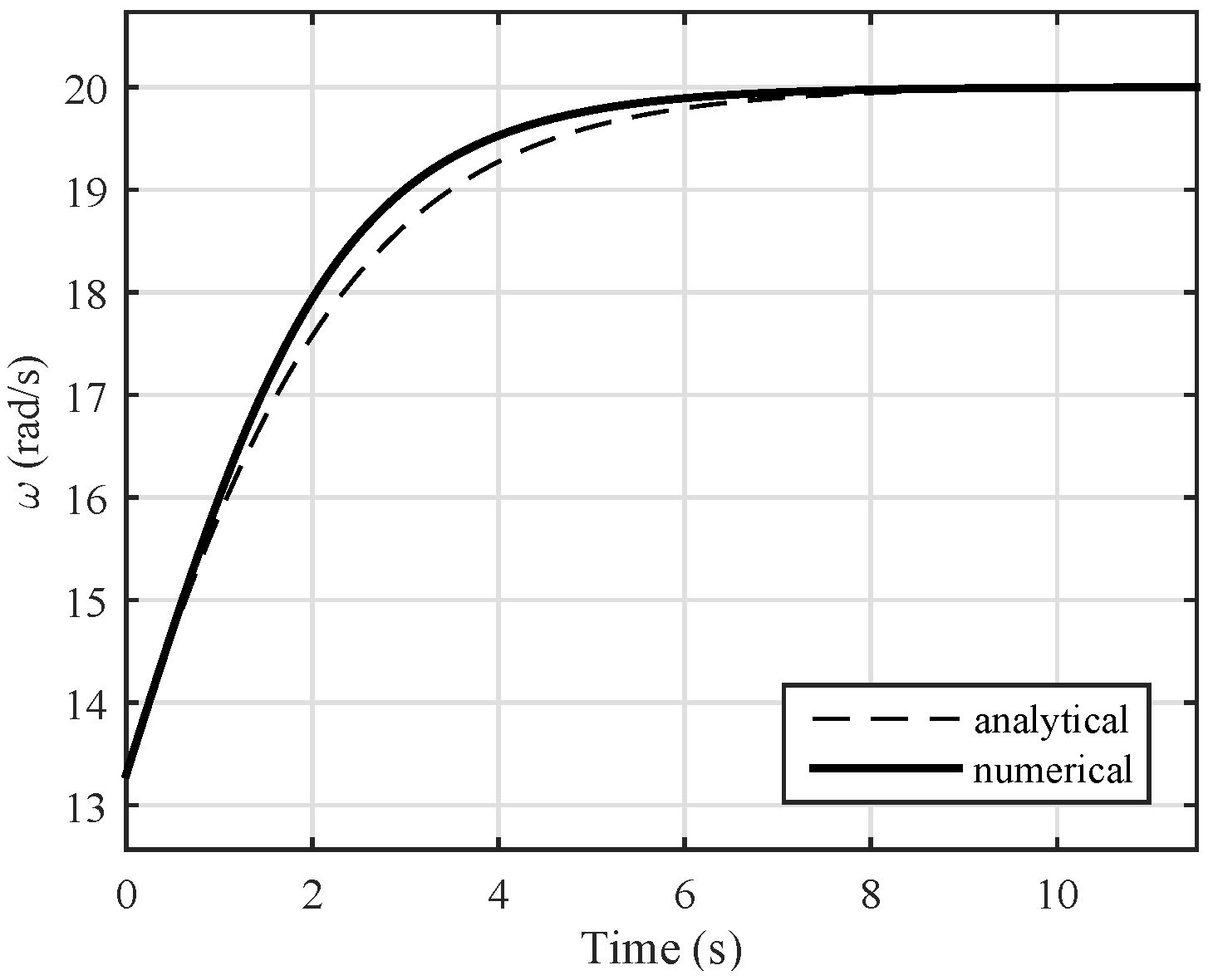
Uppsala University operates a three-bladed vertical axis wind turbine rated at 12 kW for research purposes. It operates at a nominal speed of 127 rpm (13.3 rad/s) in 12 m/s winds. Details of the turbine and generator can be found in [8]. The maximum power coefficient C is 0.29, and the runaway speed is estimated to 191 rpm (20.0 rad/s). The moment of inertia is 240 kg·m [9]. From these data, k and k could be obtained. k was assumed to be negligible and set to 0, and k and k were taken from the Söderfors turbine as mentioned.
The results are plotted in Figure 10. There is no overshoot of the runaway speed. Initially, the analytical and numerical models agree very well on the acceleration of the rotor. The analytical model then underestimates the acceleration (compared to the numerical model), since it does not take into account the time lag in wake development and, consequently, reaches runaway speed slightly later than the numerical model.
4.5. Discussion
We have assumed fixed-pitch turbine blades. The Söderfors turbine, on which the experiments were made, has fixed blades. For a variable-pitch turbine, the effects of runaway might be mitigated by active control or by feathering the turbine blades. However, the high accelerations involved may lead to a sequence of events too fast for the control system to react. It is also conceivable that, in the case of accidental load loss, the control system is itself rendered inoperable. Either way, any influence due to blade pitching would serve to lower maximum forces, and so, the models might still provide an upper estimate of speeds and accelerations.
The turbine mass moment of inertia J includes any added inertia, but is assumed to be constant. This is a simplification, since added mass will vary with acceleration during runaway.
The models were derived without any assumptions regarding turbine type in terms of axis orientation. The example shown in Section 4.3 shows that the model may be applied to horizontal axis turbines, just as well as to vertical axis turbines. In the example, we adjusted the values of J, k and k to fit the desired results, but better knowledge of the particular turbine would be required to model it properly.
In applying the models to a vertical axis wind turbine (Section 4.4), we hypothesised that k and k for the Söderfors turbine could be applied. This needs further investigation, since there are obvious differences between the turbines, even though they are both of the vertical axis type. For example, the number of blades is different and so is the aspect ratio (proportion of turbine diameter to blade height). Both of these parameters, as well as others, may conceivably influence the values of k and k.
The model constants also need further study in general. The experimental data available for comparisons are limited in scope to one turbine and, essentially, one freestream flow speed. Ideally, it should be verified that the constants are in fact invariant under different operational conditions. It would also be interesting to obtain values of the constants for various turbines. Typical values for different turbine types could possibly be determined in this manner.
The models are concerned with the development over time of angular velocity with no electrical load connected. With the experimental setup used, the simplifications outlined in Section 2 (no copper losses and only constant iron losses) are valid. In principle, it would be easy to include a load term in Equations (32) and (33) in order to study turbine behaviour as the load is changed (but not disconnected entirely). Depending on how big a change is made, and how quickly, a turbine may or may not overshoot (or “undershoot”, if the load is increased) the new operational angular velocity. Similarly, it should be possible to model cases where the load is not disconnected so “cleanly” as in the reported experiments.
The numerical model, supported by experimental results, indicates that on runaway from standstill the runaway speed overshoot may be well over 35% (Figure 7). This has to be taken into account when designing the turbine runner and in fault analysis. If the final runaway speed is assumed to be the limiting case in terms of peak angular velocity, mechanical loads on the turbine are bound to be underestimated.
The point of predicting accelerations and peak angular velocities is to estimate forces to which the turbine is subjected. Better understanding of angular speed development may also aid in the analysis of wake speed evolution. Calculation of these forces and wake velocity fields is beyond the scope of the current paper.
5. Conclusions
We have constructed two models of turbine runaway behaviour, one analytical and one numerical. Comparisons with measured data from a vertical axis marine current turbine show that both models give reasonably accurate estimates of initial acceleration and that the numerical model captures the phenomenon of runaway speed overshoot well in terms of magnitude and timing. By comparison with published data, we have also been able to indicate that the models should be able to handle horizontal axis turbines just as well. A test run modelling a vertical axis wind turbine also produced expected results in that no overshoot was observed for that turbine.
Turbine behaviour during runaway and, in particular, the phenomenon of runaway speed overshoot in marine current turbines, requires more attention than it has been getting so far. The models presented in this paper can be further developed for these purposes. Using the models to estimate forces on the turbine is a natural next step to study.
Acknowledgments
The work reported was financially supported by Vattenfall AB, the Swedish Research Council, the ÅForsk Foundation, StandUp for Energy, the Swedish Energy Agency (Swedish Centre for Renewable Electric Energy Conversion, CFE III), the J. Gust. Richert Memorial Fund and the Bixia Environmental Fund.
Author Contributions
Staffan Lundin developed the models, participated in the experiments and wrote the manuscript. Anders Goude initiated and participated in the experiments and contributed to the writing. Mats Leijon supervised the work.
Conflicts of Interest
The authors declare no conflict of interest.
Abbreviations
| rad/s | Angular velocity of turbine | |
| rad/s | Initial angular velocity | |
| rad/s | Peak angular velocity | |
| rad/s | Operational angular velocity | |
| rad/s | Runaway angular velocity | |
| rad/s | Nominal angular velocity | |
| u | m/s | Flow speed |
| u | m/s | Freestream flow speed |
| u | m/s | Flow speed seen by turbine |
| u | m/s | u in steady operation |
| u | m/s | Flow speed in the far wake |
| u | m/s | u when turbine is at |
| u | m/s | u when turbine is at |
| u | m/s | Flow speed at turbine runner |
| k | kg·m | Constant associated with hydrodynamic driving torque |
| k | kg·m | Constant associated with hydrodynamic torque loss |
| k | N·m | Torque loss constant |
| k | - | Steady speed constant |
| k | - | Operational volume size constant |
| t | s | Time at which occurs |
| s | Time between zero-crossings | |
| f | s | Electric frequency |
| E | J | Energy |
| E | J | Kinetic energy of operational volume |
| E | J | Rotational energy of rotating system |
| Q | N·m | Torque |
| Q | N·m | Hydrodynamic torque contribution |
| Q | N·m | Constant torque loss |
| Q | N·m | Torque due to connected load |
| Q | N·m | Torque due to iron losses in stator |
| P | W | Power |
| P | W | Power dissipated in load |
| P | W | Copper losses in generator windings |
| P | W | Power delivered by turbine in steady operation |
| P | W | Electric power |
| C | - | Power coefficient |
| J | kg·m | Inertia of rotating system |
| R | m | Turbine radius |
| D | m | Turbine diameter |
| m | Turbine cross-sectional area | |
| V | m | Operational volume |
| kg/m | Mass density of flow | |
| - | Tip speed ratio | |
| C | - | Constant of integration |
References
- Faudot, C.; Dahlhaug, O.G.; Holst, M.A. Tidal Turbine Blades in Runaway Situation: Experimental and Numerical Approaches. In Proceedings of the 10th European Wave and Tidal Energy Conference (EWTEC13), Aalborg, Denmark, 2–5 September 2013.
- Winter, A.I. Differences in Fundamental Design Drivers for Wind and Tidal Turbines. In Proceedings of the OCEANS 2011 IEEE-Spain, Santander, Spain, 6–9 June 2011; pp. 1–10.
- Hosseinimanesh, H.; Devals, C.; Nennemann, B.; Guibault, F. Comparison of steady and unsteady simulation methodologies for predicting no-load speed in Francis turbines. Int. J. Fluid Mach. Syst. 2015, 8, 155–168. [Google Scholar] [CrossRef]
- Manwell, J.F.; McGowan, J.G.; Rogers, A.L. Wind Energy Explained: Theory, Design and Application, 2nd ed.; Wiley: Chichester, UK, 2009. [Google Scholar]
- Eriksson, S.; Bernhoff, H. Loss evaluation and design optimisation for direct driven permanent magnet synchronous generators for wind power. Appl. Energy 2011, 88, 265–271. [Google Scholar] [CrossRef]
- Yuen, K.; Lundin, S.; Grabbe, M.; Lalander, E.; Goude, A.; Leijon, M. The Söderfors Project: Construction of an Experimental Hydrokinetic Power Station. In Proceedings of the 9th European Wave and Tidal Energy Conference (EWTEC11), Southampton, UK, 5–9 September 2011; pp. 1–5.
- Lundin, S.; Forslund, J.; Carpman, N.; Grabbe, M.; Yuen, K.; Apelfröjd, S.; Goude, A.; Leijon, M. The Söderfors Project: Experimental Hydrokinetic Power Station Deployment and First Results. In Proceedings of the 10th European Wave and Tidal Energy Conference (EWTEC13), Aalborg, Denmark, 2–5 September 2013.
- Kjellin, J.; Bülow, F.; Eriksson, S.; Deglaire, P.; Leijon, M.; Bernhoff, H. Power coefficient measurement on a 12 kW straight bladed vertical axis wind turbine. Renew. Energy 2011, 36, 3050–3053. [Google Scholar] [CrossRef]
- Deglaire, P.; Eriksson, S.; Kjellin, J.; Bernhoff, H. Experimental Results from a 12 kW Vertical Axis Wind Turbine with a Direct Driven PM Synchronous Generator. In Proceedings of the European Wind Energy Conference & Exhibition (EWEC 2007), Milan, Italy, 7–10 May 2007.
Figure 1.
Example of angular velocity development according to the analytical model.
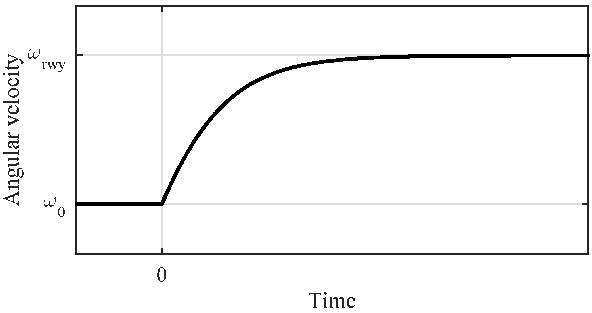
Figure 2.
Wake speed measurements re-computed as flow speed at turbine and fitted curve.

Figure 3.
Examples of numerical results for different values of k.

Figure 4.
Comparison of model predictions with measured results. Cases are specified in Table 3.
Figure 4.
Comparison of model predictions with measured results. Cases are specified in Table 3.

Figure 5.
Comparison of time derivatives of model predictions and measured results. Cases are specified in Table 3.
Figure 5.
Comparison of time derivatives of model predictions and measured results. Cases are specified in Table 3.

Figure 6.
Initial and maximum accelerations predicted analytically and numerically.
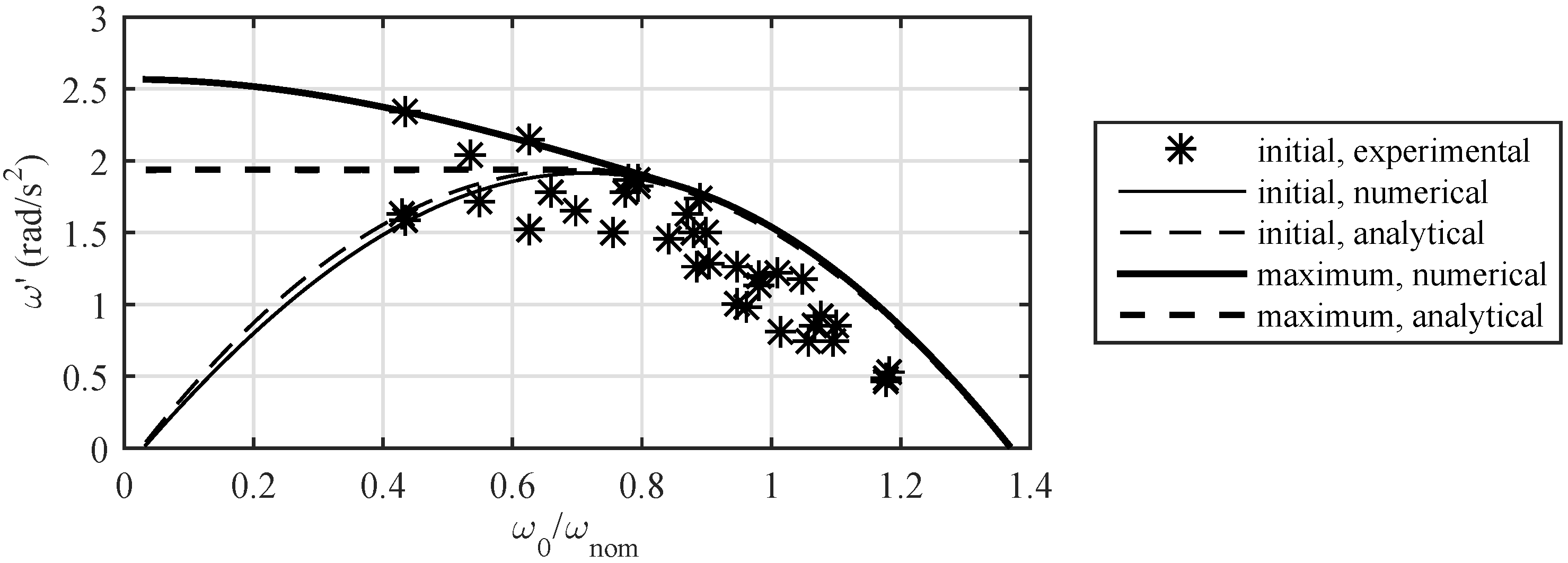
Figure 7.
Maximum angular velocity overshoot normalized by runaway angular velocity.
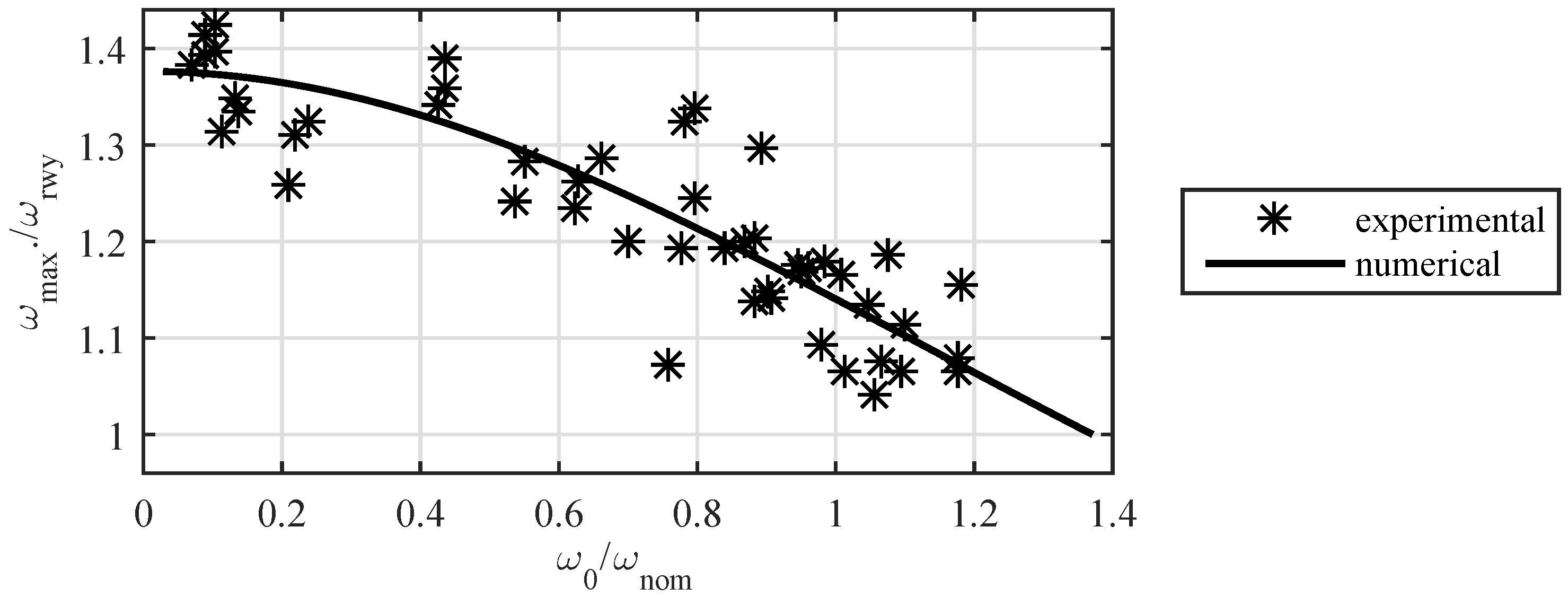
Figure 8.
Time of maximum overshoot in seconds from release.

Figure 9.
An attempt at recreating the plot in Figure 6 of [1]. Crosses mark points on the experimental curve, taken from that figure by hand measurement.
Figure 9.
An attempt at recreating the plot in Figure 6 of [1]. Crosses mark points on the experimental curve, taken from that figure by hand measurement.
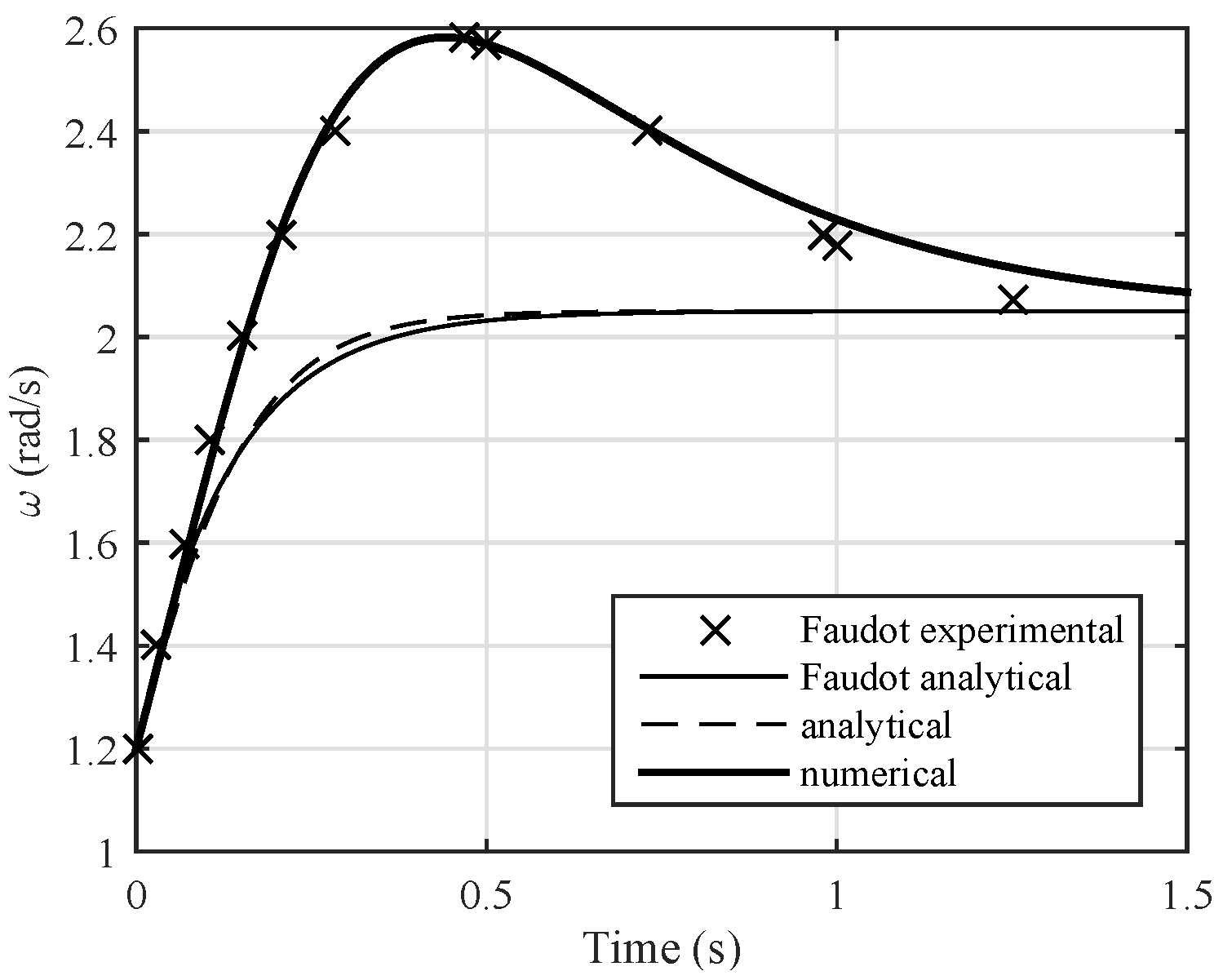
Figure 10.
Runaway development of a 12-kW vertical axis wind turbine.


| Parameter | Value | |
|---|---|---|
| Turbine runner | Number of blades | 5 |
| Hydrofoil | NACA0021 | |
| Blade chord length | 0.18 m | |
| Blade height | 3.5 m | |
| Diameter | 6.0 m | |
| Generator | Number of poles | 112 |
| Nominal frequency | 14 s | |
| Winding resistance | 0.324 Ω/phase | |
| Iron loss torque | 110 N·m | |
| Rotating system | Mass moment of inertia | 3 000 kg·m |
| Mechanical torque loss | 350 N·m | |
| Nominal operation | Water flow speed | 1.4 m/s |
| Rotational speed | 15 rpm | |
| Angular velocity | 1.57 rad/s | |
| Output power | 7.5 kW | |
| Quantity | Value | |
|---|---|---|
| Freestream flow speed u | 1.42 m/s | |
| With load connected | Power P | 7 340 W |
| Angular velocity | 1.55 rad/s | |
| Without load (runaway) | Angular velocity | 2.15 rad/s |
| Cases | Unit | Note | (a) | (b) | (c) | (d) | |
|---|---|---|---|---|---|---|---|
| Modelling conditions | Initial angular velocity | rad/s | - | 0.052 | 1.21 | 1.49 | 1.85 |
| Normalized | - | - | 0.033 | 0.773 | 0.947 | 1.18 | |
| Freestream speed u | m/s | - | 1.43 | 1.41 | 1.41 | 1.40 | |
| Results | Initial acceleration | rad/s | Experimental | 0.281 | 1.77 | 1.01 | 0.528 |
| rad/s | Analytical | 0.045 | 1.90 | 1.63 | 0.894 | ||
| rad/s | Numerical | 0.024 | 1.87 | 1.60 | 0.801 | ||
| Peak angular velocity | rad/s | Experimental | 2.98 | 2.61 | 2.47 | 2.30 | |
| rad/s | Numerical | 2.98 | 2.60 | 2.47 | 2.25 | ||
| Relative runaway speed | - | Experimental | 1.38 | 1.21 | 1.15 | 1.07 | |
| Overshoot | - | Numerical | 1.38 | 1.21 | 1.14 | 1.05 | |
| Time of peak angular velocity | s | Experimental | 2.04 | 1.47 | 1.63 | 1.43 | |
| From release t | s | Numerical | 3.00 | 1.57 | 1.56 | 1.60 | |
© 2016 by the authors; licensee MDPI, Basel, Switzerland. This article is an open access article distributed under the terms and conditions of the Creative Commons Attribution (CC-BY) license (http://creativecommons.org/licenses/by/4.0/).
Share and Cite
MDPI and ACS Style
Lundin, S.; Goude, A.; Leijon, M. One-Dimensional Modelling of Marine Current Turbine Runaway Behaviour. Energies 2016, 9, 309. https://doi.org/10.3390/en9050309
AMA Style
Lundin S, Goude A, Leijon M. One-Dimensional Modelling of Marine Current Turbine Runaway Behaviour. Energies. 2016; 9(5):309. https://doi.org/10.3390/en9050309
Chicago/Turabian StyleLundin, Staffan, Anders Goude, and Mats Leijon. 2016. "One-Dimensional Modelling of Marine Current Turbine Runaway Behaviour" Energies 9, no. 5: 309. https://doi.org/10.3390/en9050309
Note that from the first issue of 2016, this journal uses article numbers instead of page numbers. See further details here.