In order to test the proposed model, the data, related to six-year observations (years 2004–2009) from a location in the south of Italy whose latitude and longitude are 40°48.8′, 14°20.3′ [
19], were analyzed. The years 2004–2008 were used to calibrate the model (identification period) while the year 2009 was used to validate the model (validation period). The data used represent the global horizontal solar irradiance and are available on a 10 min basis, already filtered in order to clean values deriving from measurements errors or absence of measurements. Due to the characteristics of the proposed method, the data were utilized without any
ad hoc time series pre-processing finalized to extract trends or seasonality. In the following subsections, the results of the fitting of the aforementioned data (
i.e.,
and
) are reported first. Then, the results of the application of the model for forecasting purposes are shown together with an evaluation of the method’s performance.
6.2. Forecasting Application
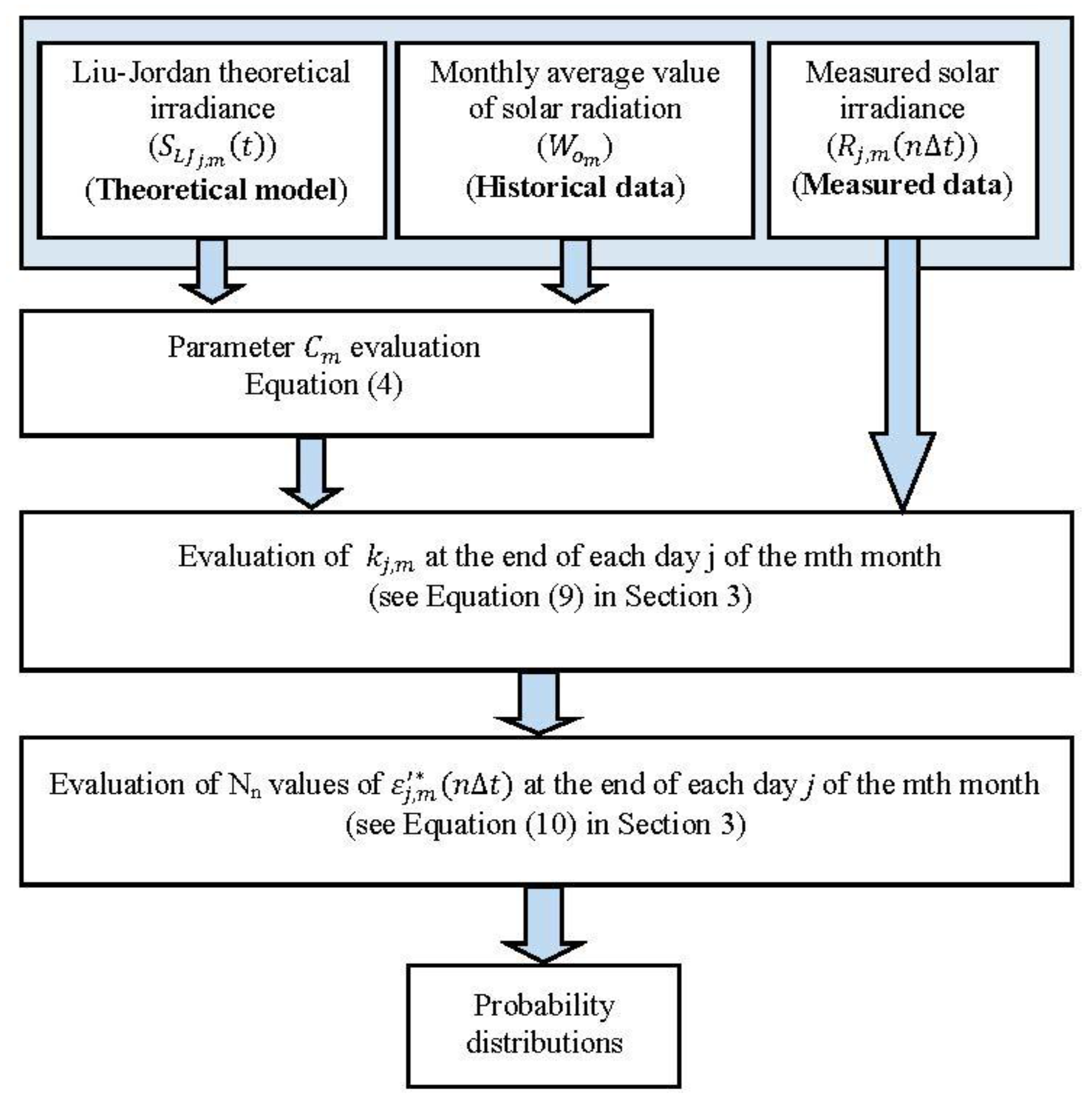
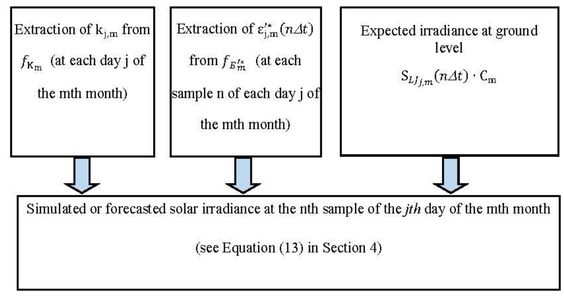
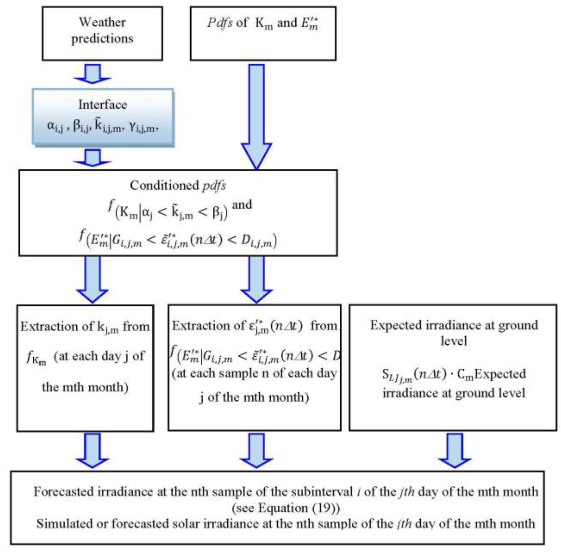
Starting from the parametric
pdfs of
and
, the forecasting procedure described in
Section 4 was applied to several tests performed with reference to all months of the year. For the sake of brevity, in what follows, only the results referring to the day-ahead forecasts for the months of January, April, July, and October are reported.
The results of the application of Parametric Marginal distribution functions (PARAMETRIC) have been compared with those obtained by means of Experimental Marginal distribution functions (EXPERIMENTAL) [
18] and the Persistence method (PERS, one of the most commonly used reference methods [
23]).
In order to compare the forecast methods performances, the mean average % error, MAE
j,m, the mean bias % error, MBE
j,m, and the root mean square % error, RMSE
j,m, have been calculated for each day of the
mth month:
with MR
j,m being the daily mean value of the measured solar irradiance evaluated over the N
s,j,m samples of the day with solar irradiance different from zero:
Skill Scores, evaluated with reference to the Persistence method of MAE and RMSE, have been also evaluated by means of the following expressions where METH refers either to EXPERIMENTAL or PARAMETRIC forecasting methods:
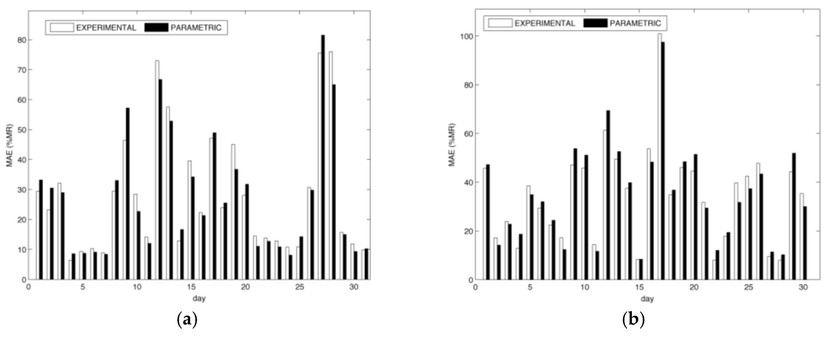
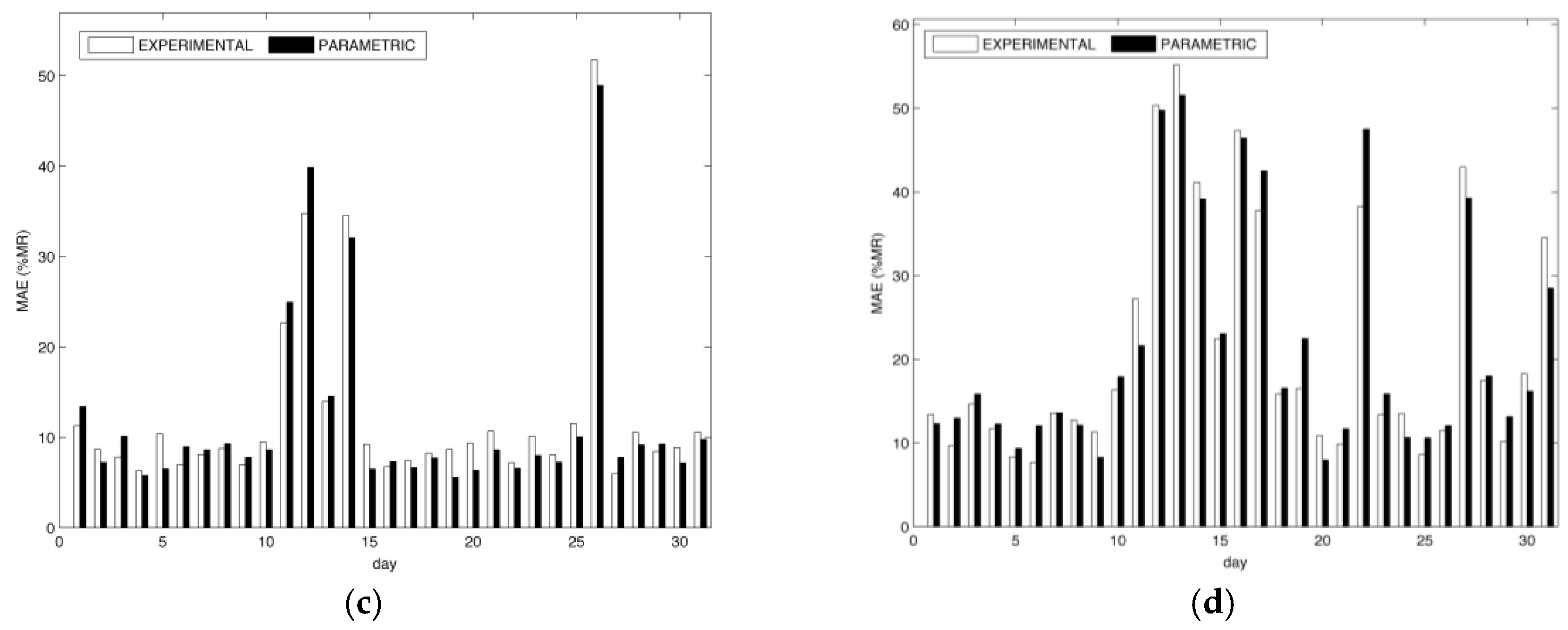
Figure 7 reports MAE
j,m values for the two different forecast methods with reference to each day of: (
a) January, (
b) April, (
c) July, and (
d) October.
It is possible to observe that:
For all the months considered, the daily error varies in a quite wide range (e.g., in October from less than 10% on the 20th to almost 50% on the 13th);
The performances of the methods are very close to each other.
Monthly mean values of the normalized MAE, normalized MBE, and normalized RMSE for the two methods are reported in
Table 4, together with the corresponding values for the Persistence method, for the same months considered in
Figure 7.
Table 5 reports Skill Scores obtained using the Persistence method as reference of the monthly mean of MAE
j,m and of RMSE
j,m for the months given in
Figure 7. EXPERIMENTAL refers to the use of the experimental marginal distribution functions proposed in [
18] and PARAMETRIC refers to the use of the parametric distribution functions proposed in this paper.
It is possible to observe that:
Both methods presented by the authors always have better performance than the Persistence method (
Table 4);
The use of parametric distributions gives almost the same performance as the experimental distributions (
Table 4);
Skill Scores for both MAE and RMSE quantify the improvement of the performance with respect to the Persistence method (
Table 5);
The performance of the proposed methods is also better for the month of July, when more stable weather conditions allow the Persistence method to have good performance (
Table 5).
Going back to
Figure 7, it is possible to observe that only some days of the month show MAE values appreciably higher than the rest of the month. In fact, looking at the monthly mode values of the MAE metric reported in
Table 6 for the four months analyzed, it is evident that the mode values are appreciably lower than the mean values (see
Table 4).
In order to understand the reason why high error values appear in some specific days (see
Figure 7), the solar irradiance on such days has been further analyzed.
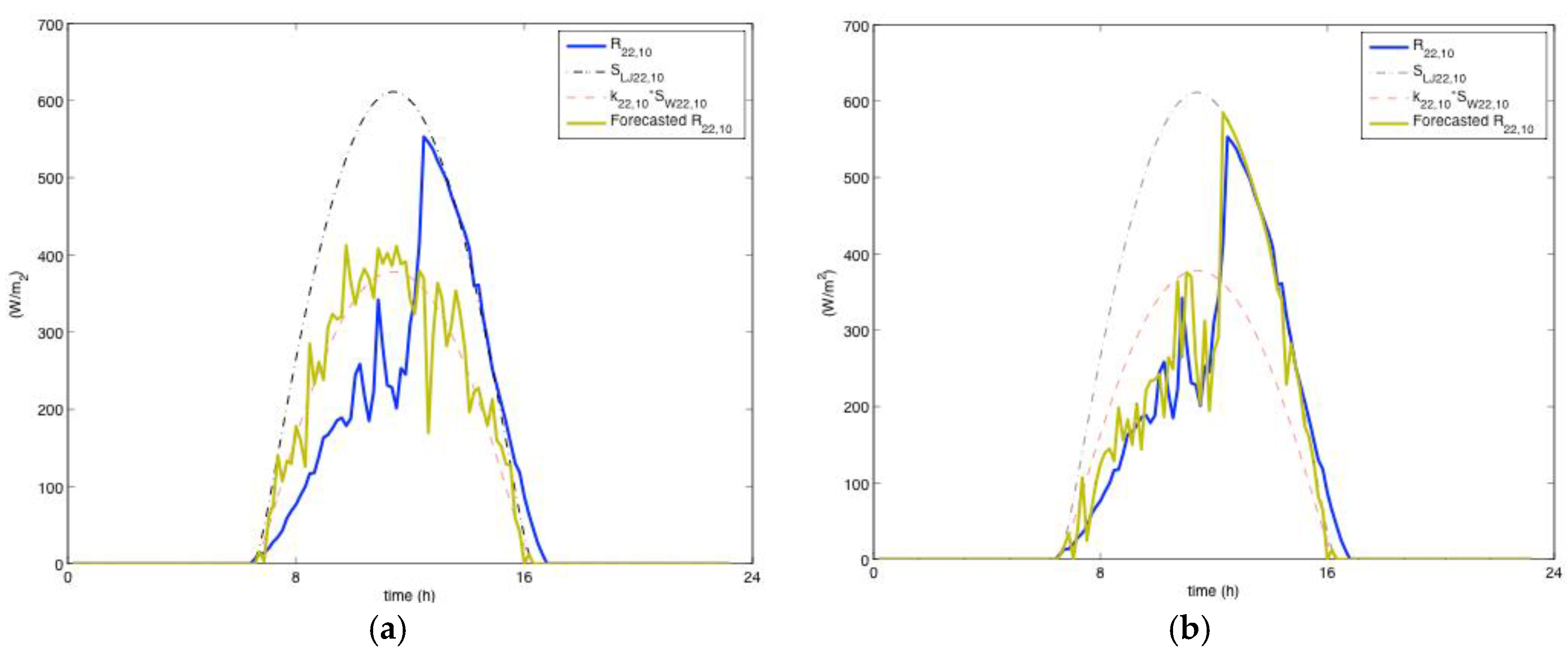
As an example,
Figure 8a reports, with reference to the 22nd of October (that is, one of the days characterized by a high error value), the measured solar irradiance,
R22,10, the forecasted solar irradiance,
, the expected clear sky theoretical solar irradiance,
SLJ22,10, and the product of the factor,
k22,10 by
SW22,10 versus the time. It is evident that the daily radiation is lower than that expected from the historical data available for the specific site (
k22,10 is lower than 1); furthermore, 2/3 of daylight hours are characterized by very low irradiance values while the remaining 1/3 of the time is characterized by high values. So this particular day is characterized by a very strong correlation between the k and ε values. This highlights an intrinsic limitation of purely statistical forecasting, which is able to follow the average behavior of the solar irradiance but randomly generates statistically independent epsilon values through the whole daylight period.
It is worth noting that the behavior of the analyzed 22nd of October helps us understand the reason why the values of the monthly modes are lower than those of the monthly means (
Table 4). In fact, looking at
Figure 7, it is possible to note that the majority of the days for all months are characterized by low error (resulting in a low value of the monthly mode) while only some days of all the months are characterized by very high error, resulting in an increased value of the monthly mean.
Results with a sensibly higher level of accuracy were obtained by applying the procedures described in
Section 5, which is able to take into account weather predictions.
Figure 8b reports the results referring to the 22nd of October obtained from the study of weather predictions able to predict the two-time behavior of the day, with a level of approximation of
of ±10%.
The figure gives an immediate visual idea of the improvement in forecasting solar irradiance through the hours of the day; the corresponding MAE
22,10 results reduced to 10% from the initial value 47% of
Figure 8d). As for the other two metrics introduced, MBE
22,10 remains almost constant around 5% while RMSE
22,10 results reduced to 13% from 58%. By analysis of the figure, the strength of the procedures shown in
Section 5 clearly appears to be predicting the different behavior during the day, not only in terms of radiation level but also in terms of variability of instantaneous solar irradiance. The first part of the day, in fact, is characterized by low values of mean solar irradiance (low
1,22,10, see Equation (16)) and a significant variability value. The second part of the day, instead, is characterized by a regular profile of the solar irradiance with a high value of mean solar irradiance (high
2,22,10 , see Equation (16)). This behavior is quite well captured by the forecasting procedure, of which the accuracy is evident, especially in case of accurate weather predictions.
This shows the difference between a purely statistical method (without taking into account any weather predictions) and the procedure completed with information on weather conditions. The former seems to be a practical solution for simulating synthetic time series in the long run (e.g., for isolated microgrids design purposes). The last seems to be a practical solution especially for those applications where information on instantaneous variations of solar irradiance is required (e.g., for day-ahead forecasts).
For comparative purposes, the results of the proposed model have been compared with the evaluations performed in [
24], which refer to a benchmarking exercise organized within the framework of the European project “WIRE” [
25] with the purpose of evaluating the performance of state-of-the-art models for short-term renewable energy forecasting. More specifically, 10 different solar power forecasting methods were applied to historical data for 2010 and 2011 and with reference to the suburbs of the city of Milan in Northern Italy and to the suburban area of Catania in Southern Italy. The location analyzed in this paper (Portici, Italy) is geographically situated between these two realities. Hence, though based on different data, this non-customized comparison can give an idea of the performance of the proposed model. For the evaluation in [
24], among the metrics adopted, the MAE, normalized by the mean power (MP) measured during the test period, was reported.
Table 7 reports the forecasting methods used by the participants in the project [
25] and their error ranges in terms of MAE (%MP) for Milano (IT) and Catania (IT). Error ranges refer to minimum and maximum values regardless of the location of the best scores reported in
Figure 7 and
Figure 8 of [
24]. Mean normalized MAE (%MR) for the methods reported in
Table 4 (evaluated for the city of Portici, IT) are reported in
Table 8. The commensurateness of the proposed method with all of the analyzed approaches clearly appears.


