1. Introduction
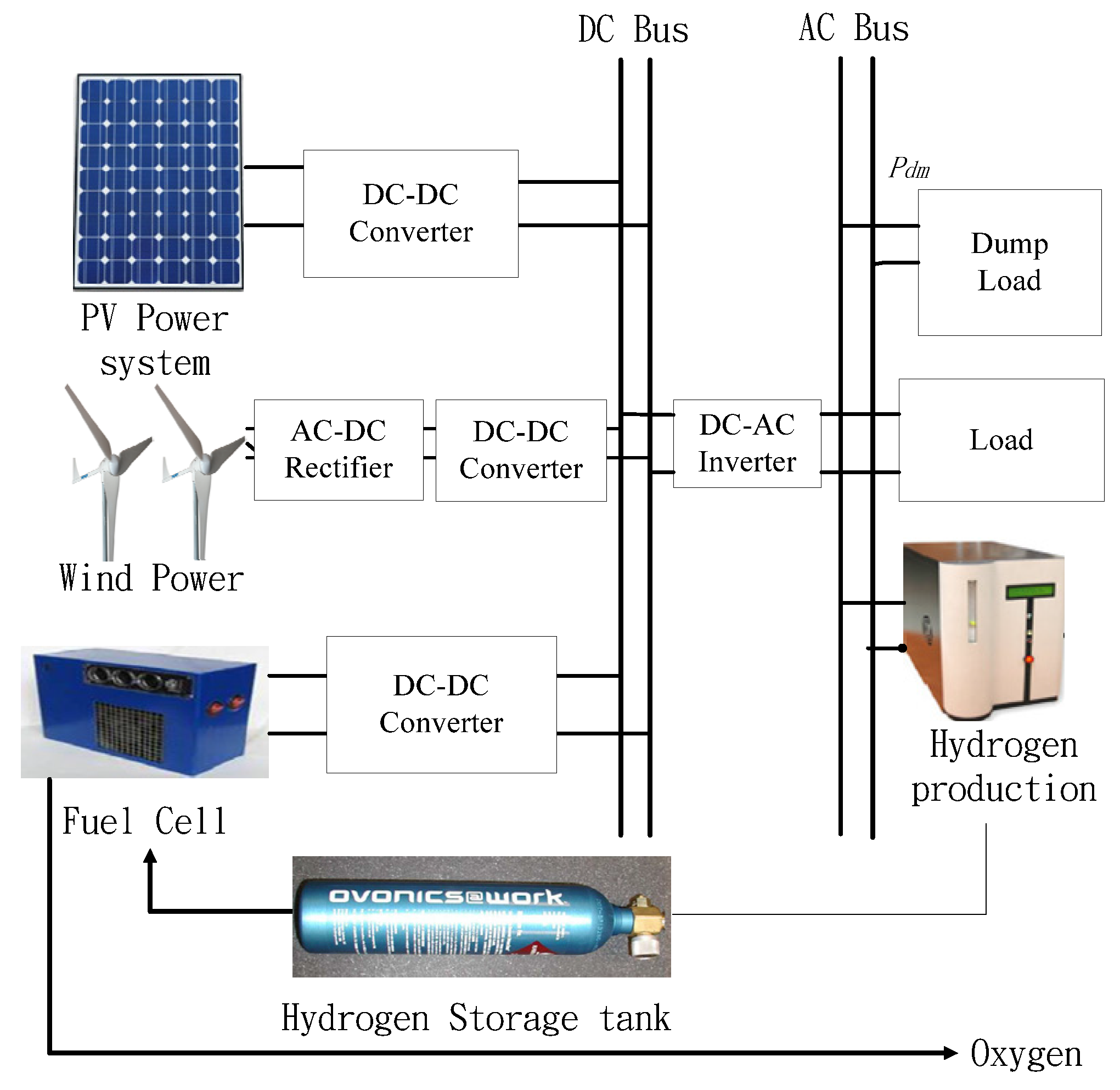
This paper integrates the renewable energy equipment of the photovoltaic (PV) power system, wind power, fuel cell, electrolyzer and hydrogen tank into one stand-alone power system. The optimized capacity allocation is an important issue for a stand-alone renewable energy system. A stand-alone renewable energy system is usually installed in remote mountains, on an island or where the utility power grid does not reach. A poor capacity allocation will not balance the power supply and demand and waste the costs for the system establishment. The simulated analysis shall be the reference of capability configuration [
1,
2]. The allocation of system device capacity affects the stand-alone power system [
3,
4]. When the device capability configuration is not appropriate, it may cause power shortages, or generate too much electricity while the system is unavailable, which wastes money [
5,
6]. On the contrary, with reasonable system allocation, the operation of power supply system will be set at the optimum cost.
Nelson
et al. applied particle swarm optimization on the optimal sizing of a stand-alone wind/fuel cell power system [
7]. They presented the unit sizing and cost analysis of stand-alone hybrid wind/PV/fuel cell power generation systems. Ekren
et al. [
8] used simulated annealing method for the size optimization of a PV/wind hybrid energy conversion system with battery storage. The drawback of this method is that it takes too much computing time and the computing results needs to be adjusted through experience to fit in the specifications of the common practical products.
Yang
et al. [
9] applied genetic algorithm to calculate the optimal system configuration with relative computational simplicity. Some commercial software like HOMER [
10], IHOGA [
11] were developed to figure out the optimal allocation. Based on the simulated weather data, this study estimates the possibility of loss of load probability (LOLP) for one or more years. Taguchi quality engineering was developed and advocated by Dr. Taguchi Genichi [
12] in 1950. The orthogonal array experiment design and analysis of variance (ANOVA) were used for the analysis with a limited experimental data to effectively improve product quality [
12]. The Taguchi method is widely applied in the manufacturing field, but this study is the first to apply the Taguchi method in the optimization of hybrid power systems.
This paper combines the extension theory with the Taguchi method, selects the proper design factors and levels via the orthogonal array to greatly decrease the number of experiments to acquire the optimum experiment result through the classical domain and neighborhood domain extension to narrow down and find the optimum capability planning. The advantages of the proposed ETM include: (1) the optimization process is subject to the specifications of practical equipment; (2) fast computing speed; and (3) the results could be directly applied on the real situation.
3. Extension Taguchi Method
To optimize the allocation of equipment capacity, this paper proposes an optimization method combining extension theory and the Taguchi method. In 1983, the concept of extension theory was proposed to solve the contradictions and incompatibility problems. Based on some proper transformation, some problems that cannot be directly solved by given conditions may become easier or solvable [
17]. One of the commonly used techniques in engineering fields is the Laplace transformation. The concept of fuzzy sets is a generalization of well-known standard sets to extend their application fields. Therefore, the concept of an extension set is to extend the fuzzy logic value from [0,1] to (−∞, ∞), which allows us to define any data in the domain and has given promising results in many fields [
18,
19,
20]. Extension theory is used to calculate the comprehensive correlative degree of each group of the simulation experiment, then the analytical method average value of the Taguchi method is used to select the optimum capability configuration system and assess whether the selected group is the optimum result [
21]. If the output result is optimal, then the process is done; otherwise, the extension correlative degree shall be recalculated. The advantage of this method is the ability to find the optimum solution in the shortest time and to limit the number of experiment trials needed. The calculation steps are as described below:
Step 1. Setting the level and design
This paper selects five three-level design factors in order to conform to the basic principle of an L
18 orthogonal array. The design factors are used to reduce the power shortage probability while not ignoring the equipment cost. Thus the price is also set as a design objective. The design factor and the corresponding levels are shown in
Table 2. The five three-level design factors are wind power, PV power, hydrogen tank, fuel cell, and electrolyzer. For example, the numbers of the wind power equipment designed for three corresponding levels are 1, 2, and 3. The numbers of equipment of each level for the design factors in
Table 2 are subject to adjustment according to the setup costs, and the optimal results could be different.
Step 2. Using the proper orthogonal array
The Taguchi method significantly reduces the number of experimental configurations to be studied. Originally, there are 3
5 = 243 experiments in the full factorial design, and the L
18 orthogonal array can accommodate five three-level design factors in only 18 experiments to efficiently collect experimental results to find the optimized factor combination. The proposed L
18 orthogonal array table is shown in
Table 3.
Step 3. Calculating the initial result
According to the experimental combinations in the orthogonal array, Matlab is applied to generate the 18 different electric power generation system quantities in the stand-alone power system which could simulate 18 different systems, and calculate each electric power generation system quantity price and power shortage hours, respectively. The results are shown in
Table 3.
Step 4. Calculating the per-unit values
The simulated experiment data cannot be compared or calculated for the unit reference value difference, thus it requires per-unit value calculation to get the physical quantity relative to the reference value [
22]. The necessary equation is as shown in Equations (3) and (4).
Step 5. Establishing the matter-element
In extension theory,
N is given as the name of an object for the definition of the object, and the quantity value of its character
c is
v. The orderly combination is taken as the fundamental element describing the object, namely the matter-element. The name of the object may not be expressed by the single matter-element, but expressed by the multi-dimensional matter-element. The multi-dimensional matter-element assumes the object has
n characters respectively
c1,
c2 …
cn, and its corresponding quantity value is
v1,
v2 …
vn. Putting the above
into
v, the multi-dimensional matter-element expression is as shown in Equation (20), and the second group is placed after calculating the correlation functional value:
Step 6. Establishing the classical domain and neighborhood domain
In extension theory, the positional relation of one point to two sections must be considered. If
and
are two sections in the real domain, it shall firstly confirm the classical domain and the neighborhood domain before getting the matter-element in. Establishing the system’s matter-element model, the defined classical domain is as Equation (21) and the neighborhood domain is as Equation (22). Defining the range according to the design factor demand, in extension theory, the classical domain is the expected value, and the neighborhood domain is the overall range.
Step 7. Calculating the correlation values
According to the definition of distance, we confirm the correlation function and use Equation (23) for assessment. If the value to be measured is within the classical domain, it shall be calculated by the method of Equation (23a); if the value to be measured is outside the classical domain, it shall be calculated in the method of Equation (23b) to get the correlation function.
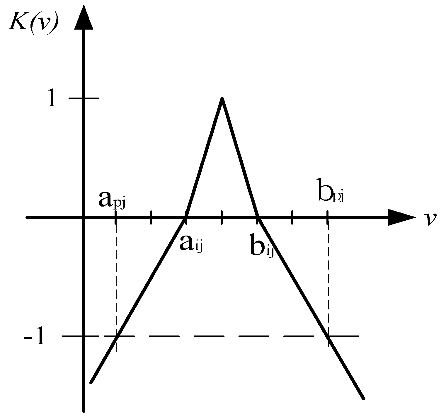
The proposed extension relation function can be shown as
Figure 5, where 0 ≤
K(
v) ≤ 1 corresponds to the normal fuzzy set. It describes the degree to which
v belong to
V. When
K(
v) < 0, it indicates the degree to which
v does not belong to
V.
Step 8. Comprehensive correlation degree
In the stand-alone power system, normally, the power shortage hours have higher priority than cost and the correlation degree function α
1 is set at 0.62 and α
2 is at 0.38 as in Equation (24), the result is given as shown in
Table 4.
Step 9. Average value analysis
Average value analysis uses the Taguchi method to calculate the influence of the factor effects to confirm the optimal factor combination by taking the average value analysis of levels for each factor by normalizing each level of comprehensive correlative degree of
Table 5 according to the
L18 orthogonal array grade in
Table 4 to calculate the average value. The average value analysis is as shown in Equation (25), and the result is as shown in
Table 6.
Step 10. Solution of optimum system parameter
Through the analysis of factor effects, the maximum stand-alone power system optimum allocation can be selected through average value analysis of the Taguchi method as shown in
Table 6.
4. Simulated Result and Discussion
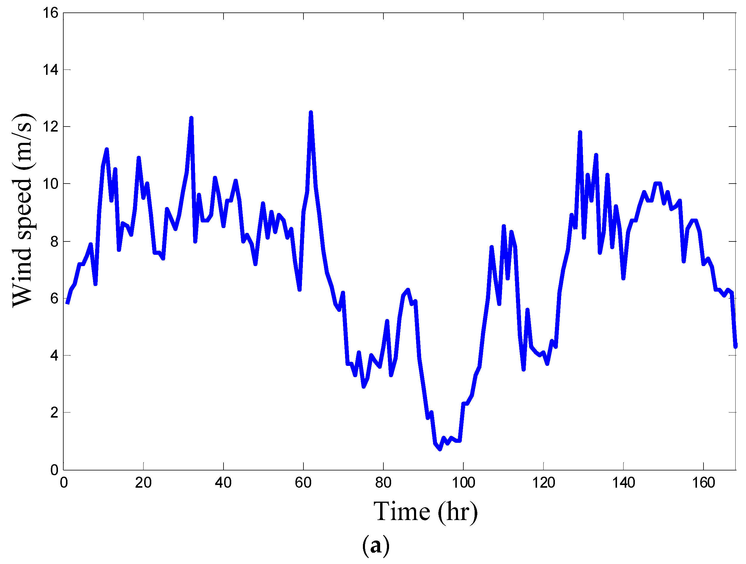
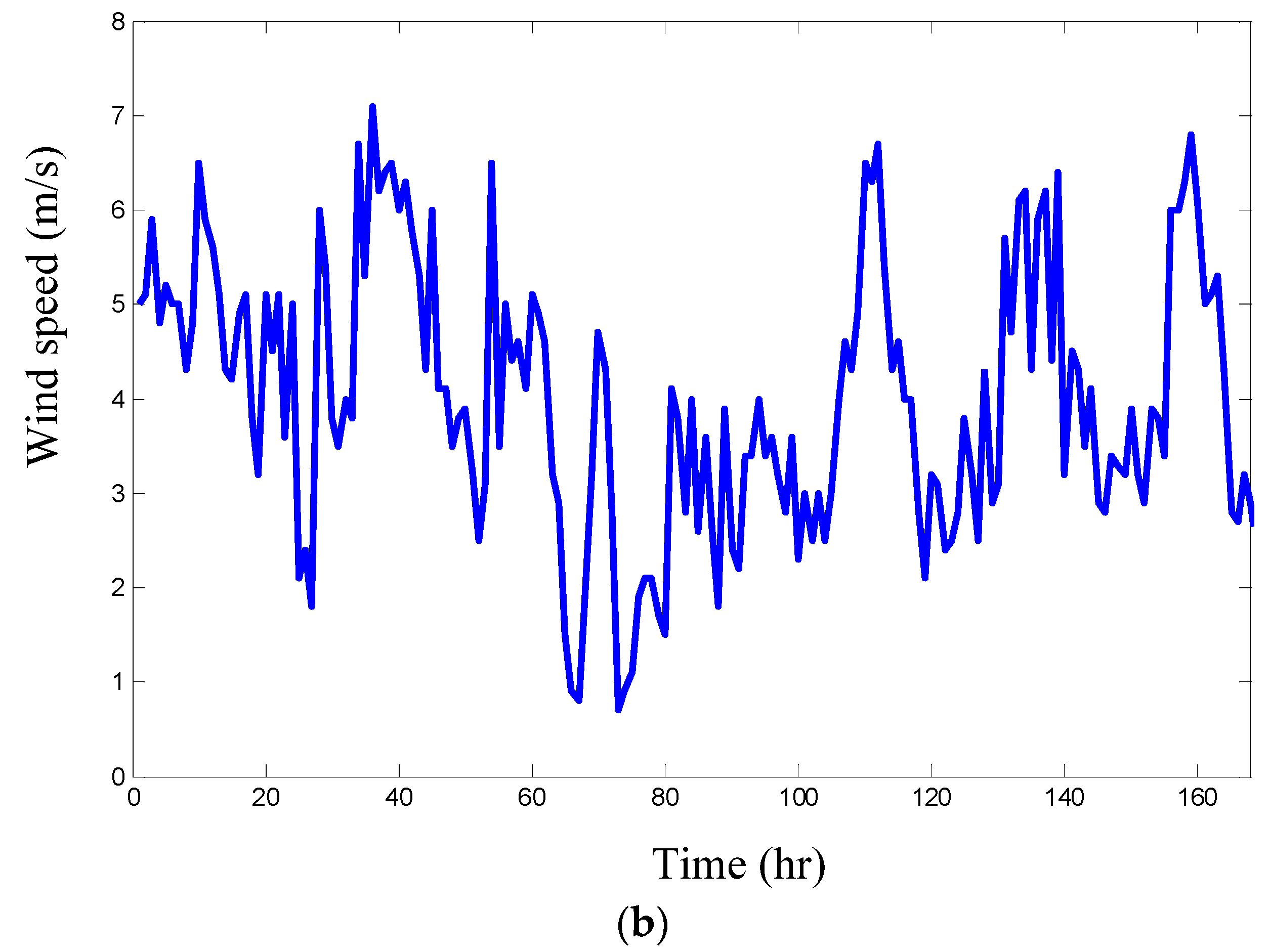
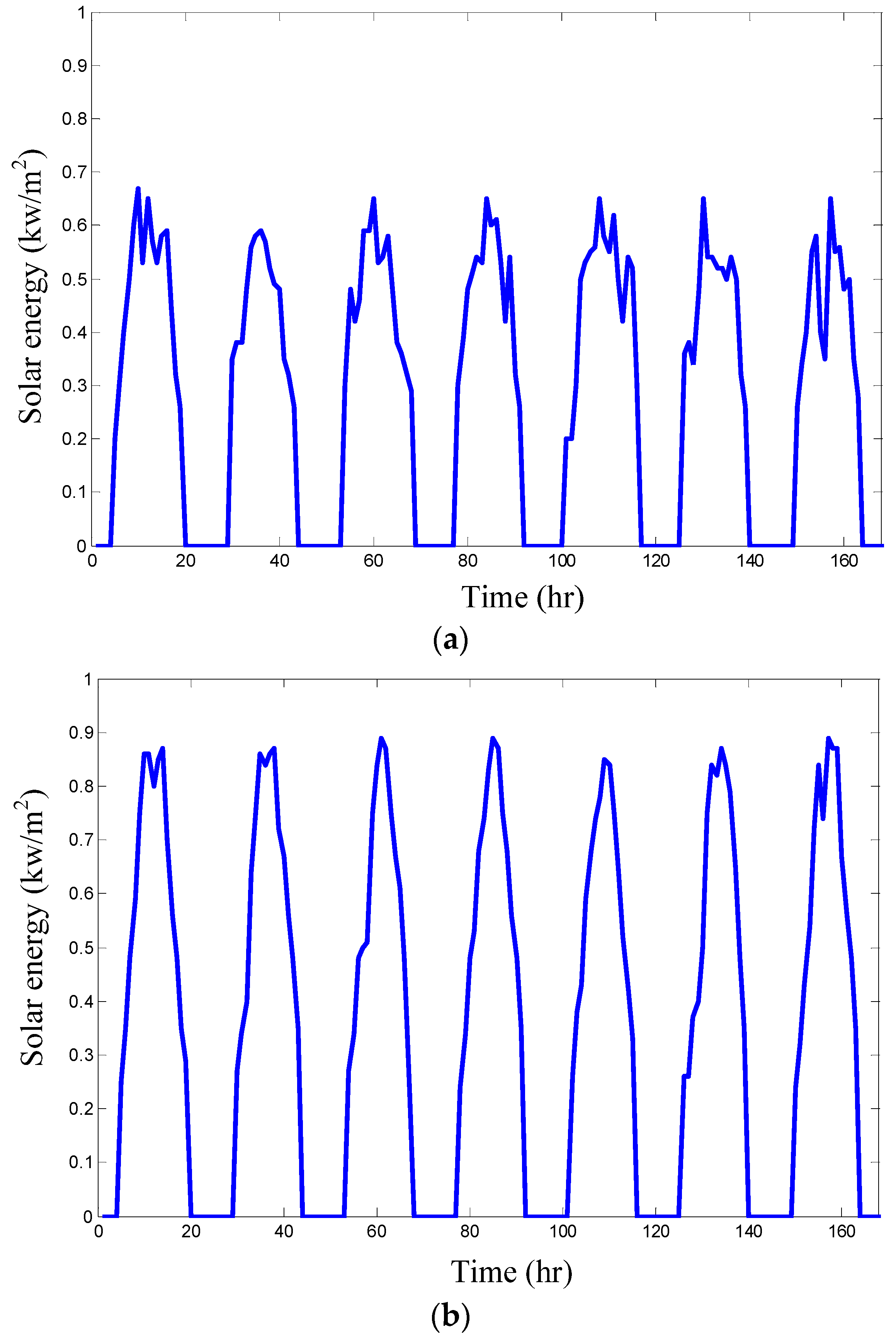
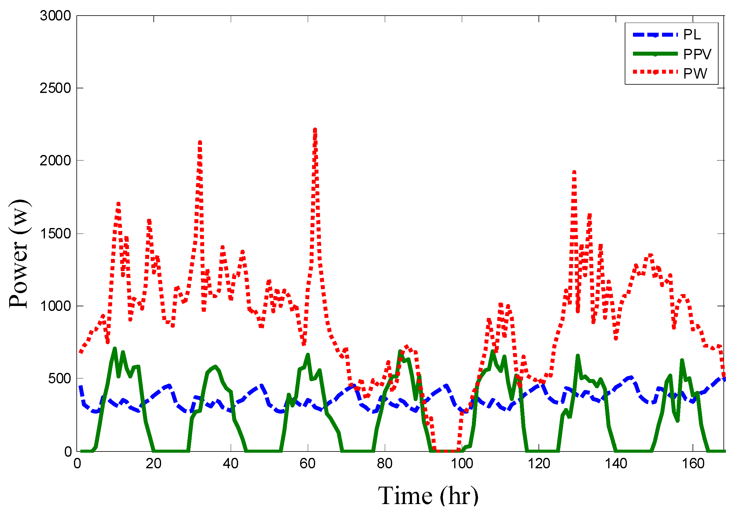
This study’s simulation adopts the weather data of the Wuci area in central Taiwan in 2014, provided by Taiwan Central Weather Bureau, to compare the wind speed and the illumination of the winter and summer, as shown in
Figure 6 and
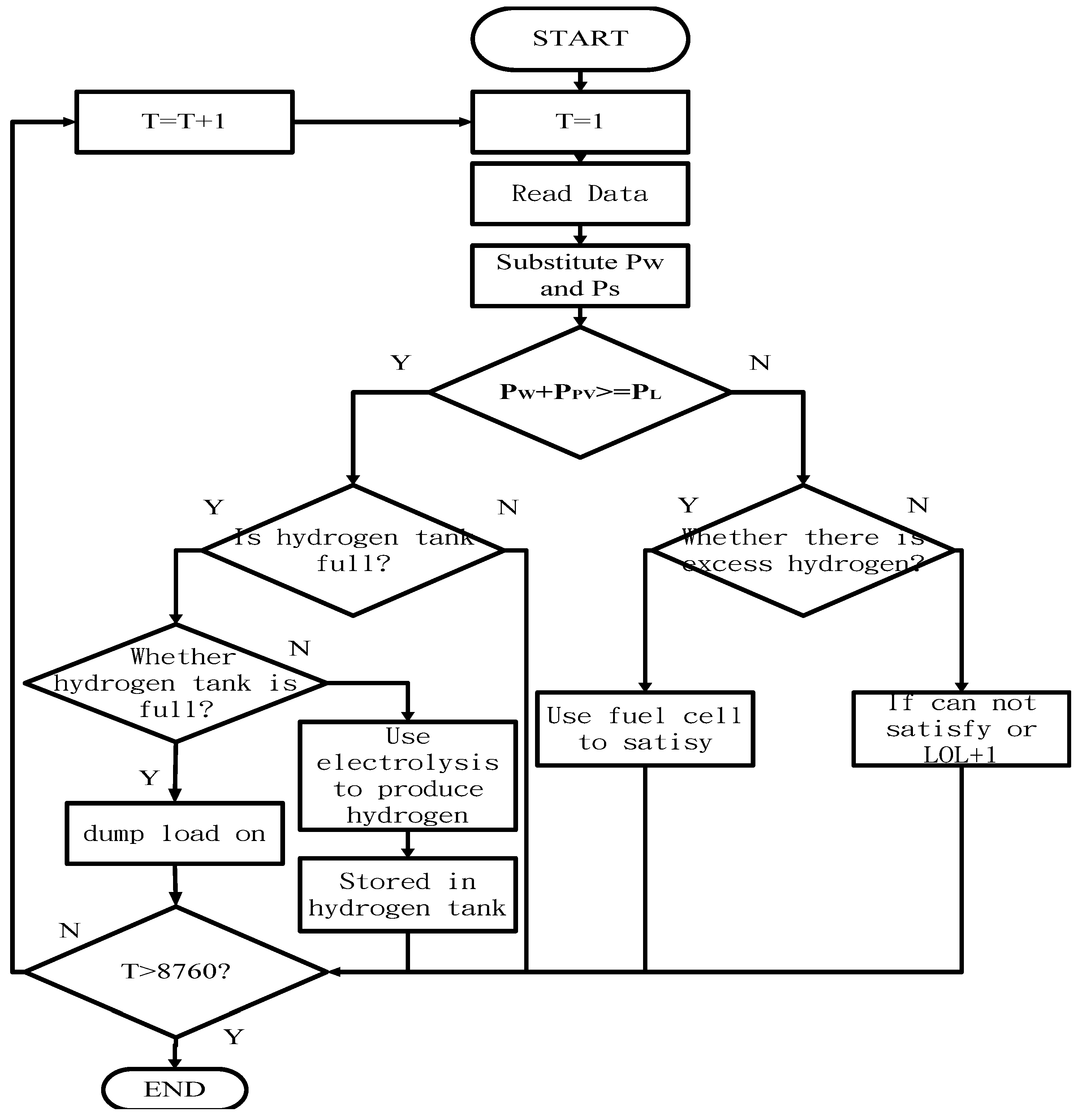
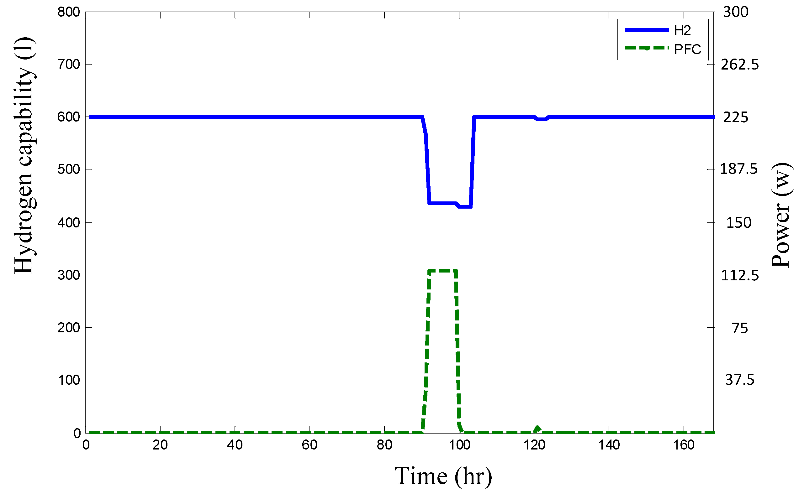
Figure 7. The sun radiates directly on the Southern Hemisphere, and the illumination is small and the wind power is strong in Taiwan. The load power (PL), wind (pw) power and PV power (PPV) of the calculated optimum allocation are shown in
Figure 8. If the amount is less than the generating capacity load, fuel cells will supply the load power, as shown in
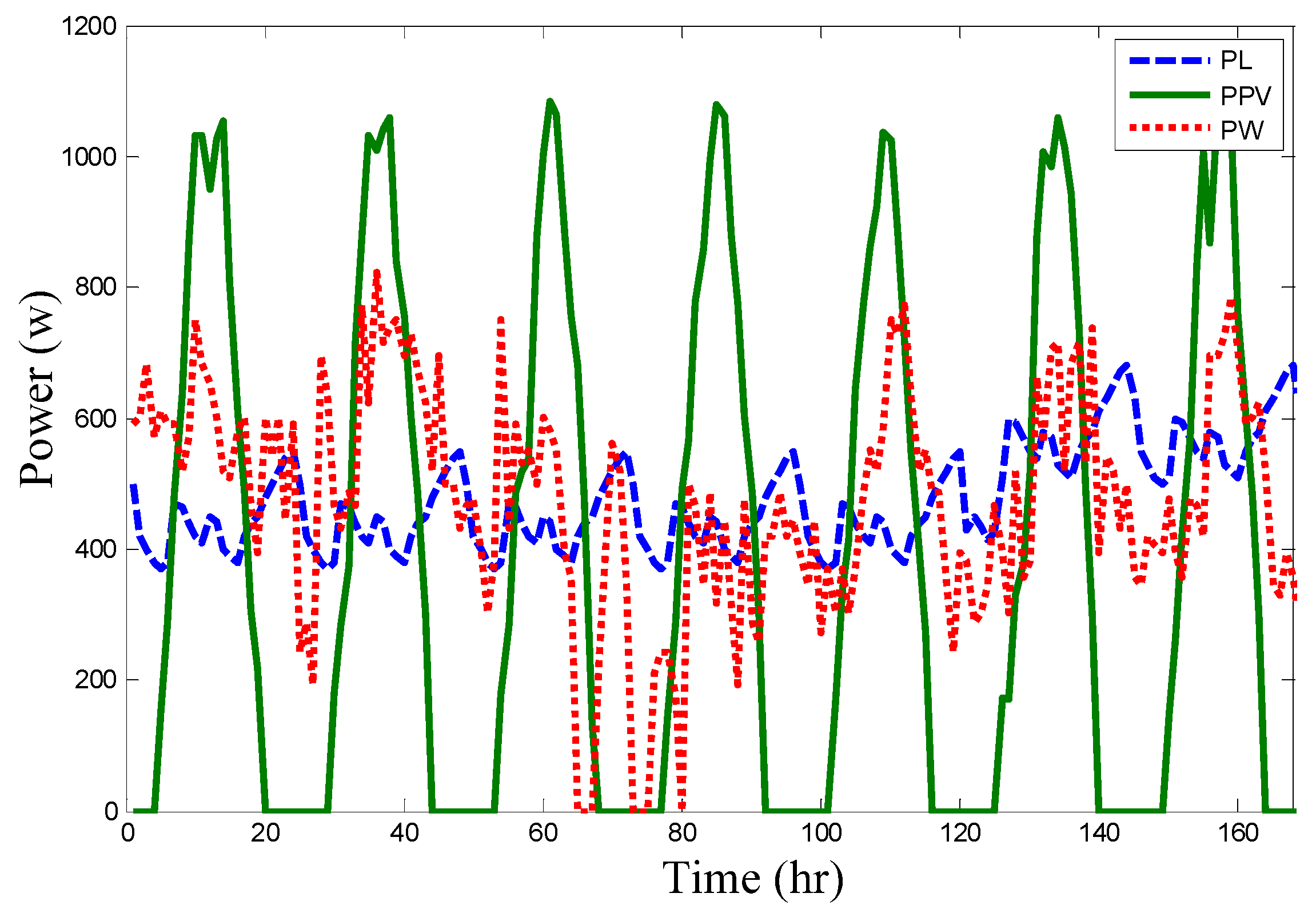
Figure 9. In summer, the load power (PL), wind (pw) power and PV power (PPV) of the calculated optimum allocation are also shown in
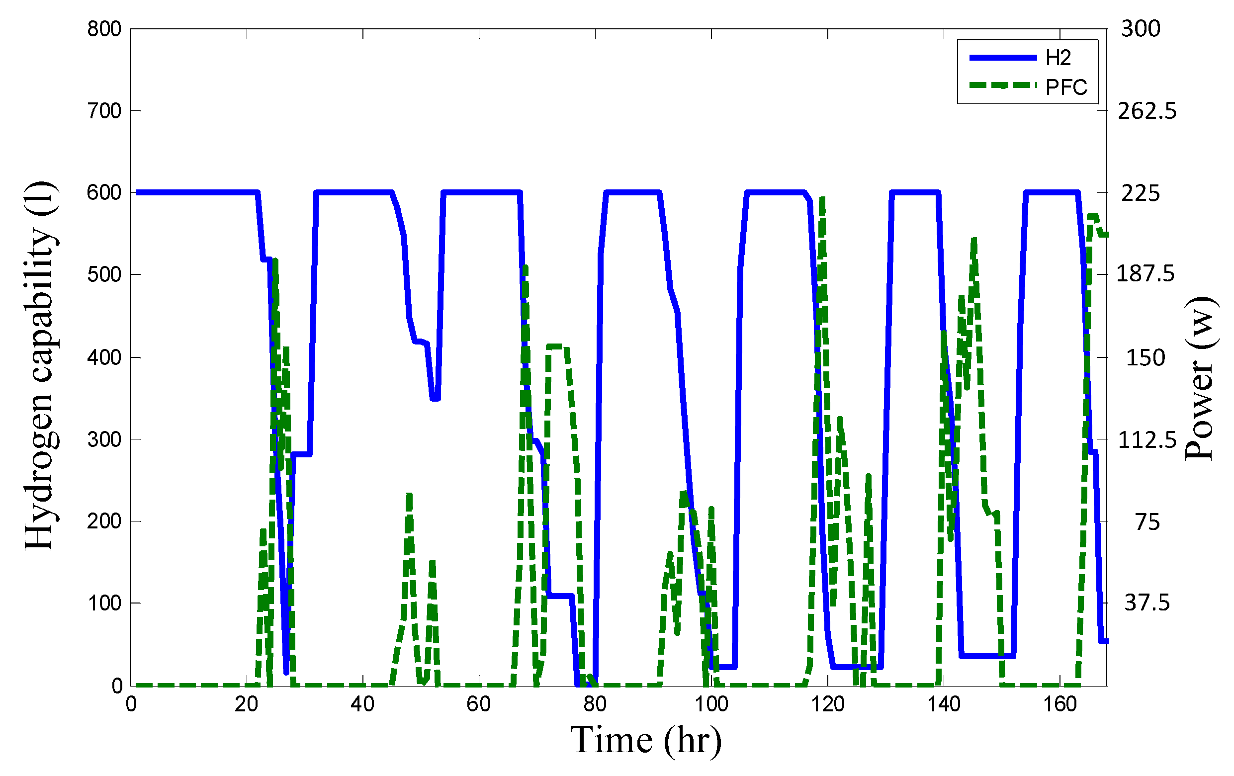
Figure 10. If the amount is less than the generating capacity load, fuel cells power will be used to supply the load, as shown in
Figure 11. In summer, the sun directly radiates on the Northern Hemisphere, the PV power increases in energy. However, there are usually windless situations in the summer, and the operation of the wind power generator is suspended during typhoon season, thus wind power generation shall decrease. Generally, during the daytime, solar energy is abundant and the use of the fuel cells is not required, and the system is able to produce hydrogen for extra needs. At night, there is no illumination, and only wind power generation provides energy. The fuel cells shall use the hydrogen to support the load. At night, in addition the home electricity usage increases, therefore, in the stand-alone power system, the fuel cell does not need much generating capacity, but needs more hydrogen tanks for standby to supplement the load demand.
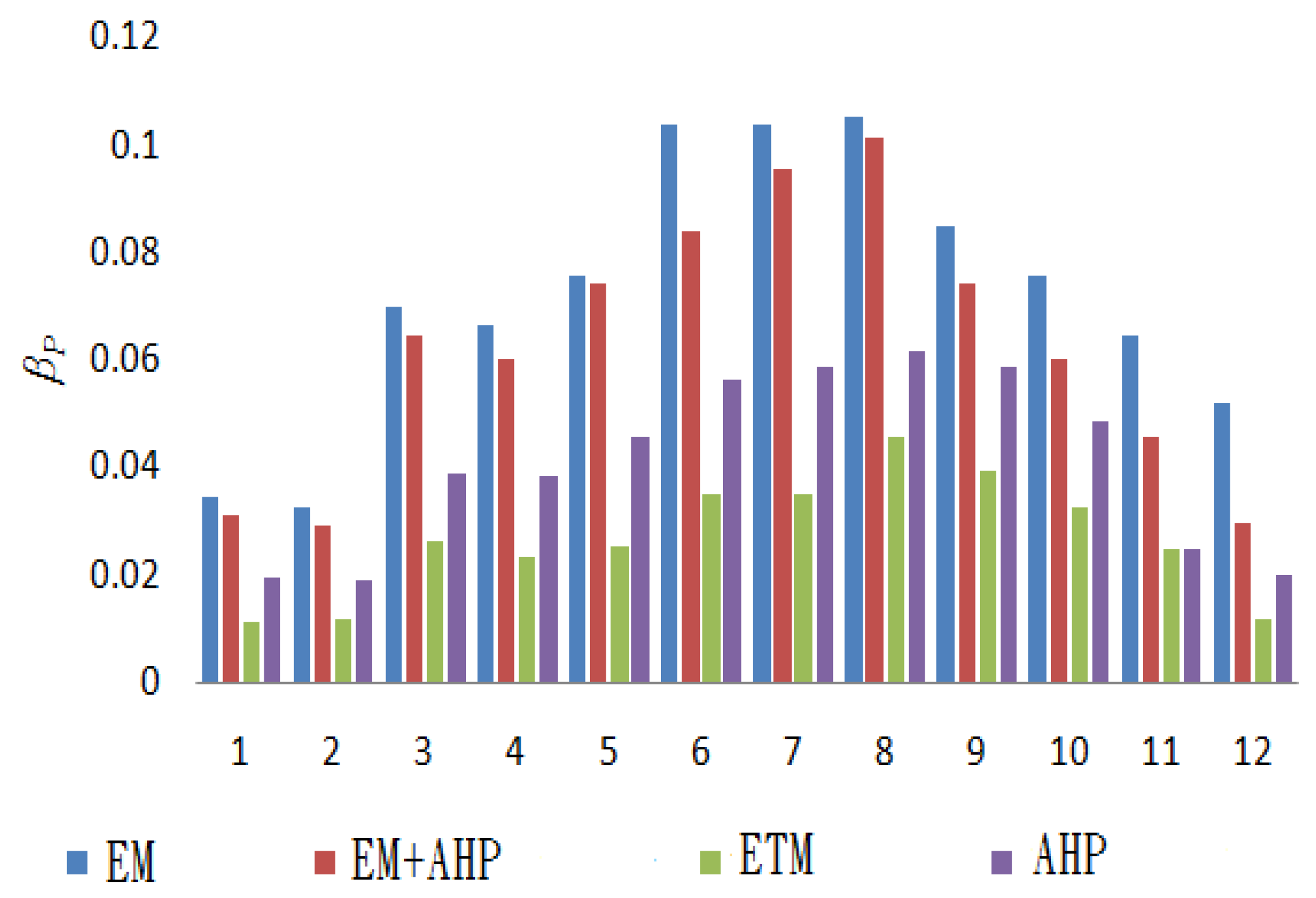
The optimum allocation into the weekly and monthly average data shall be simulated to compare the probability of shortage allocated for the four types of algorithms, as shown in
Figure 12.
The extension hierarchical method firstly adopts the extension classical domain and neighborhood domain, taking the matter-element to be measured to calculate the correlation function and extension distance, and forming the contrast matrix by the empirical law to establish hierarchical analysis method to conform to the requirement of consistency and gain weight. Comparing AHP and the Extension Taguchi Method (ETM), although the power shortage hours of AHP are good, the allocation of the ETM is better than with other optimum methods.


