Constant Jacobian Matrix-Based Stochastic Galerkin Method for Probabilistic Load Flow

Abstract

An intrusive spectral method of probabilistic load flow (PLF) is proposed in the paper, which can handle the uncertainties arising from renewable energy integration. Generalized polynomial chaos (gPC) expansions of dependent random variables are utilized to build a spectral stochastic representation of PLF model. Instead of solving the coupled PLF model with a traditional, cumbersome method, a modified stochastic Galerkin (SG) method is proposed based on the P-Q decoupling properties of load flow in power system. By introducing two pre-calculated constant sparse Jacobian matrices, the computational burden of the SG method is significantly reduced. Two cases, IEEE 14-bus and IEEE 118-bus systems, are used to verify the computation speed and efficiency of the proposed method.

1. Introduction

Load flow studies are essential for power system operators and planners, and accurate real-time load flow analysis is the basis of advanced application of modern EMS, such as optimal power flow, voltage control and so on. However, with the rapid increase in renewable energy (primarily wind and solar energy) which has strong volatility and intermittency, deterministic load flow (DLF) analysis cannot reflect the uncertainties of a power system properly. Therefore, the uncertainty of modern power grid needs to be qualified to analyze its influence on the power system.

Uncertainty quantification (UQ) [1] is the science of quantitative characterization and reduction of uncertainties in applications. It tries to determine how likely certain outcomes are if some aspects of the system are not exactly known. Probabilistic load flow (PLF) evaluation is an efficacious UQ tool to tackle the uncertainties in power systems and obtain the statistical quantities of random output variables. Traditional PLF methods can be classified into four categories: simulation methods, approximate techniques, analytical methods and heuristic procedures.

The Monte Carlo method (MCM) [2] is the most straightforward among simulation methods, but it requires DLF calculations at numerous sampling nodes even though some improvements have been proposed (such as Latin Hypercube [3] and Quasi-Monte Carlo [4] samplings). Approximate techniques provide approximate description of the statistical quantities of random output variables, and they include the point estimate method (PEM) [5], first-order second-moment method (FOSM) [6], non-parametric density estimate method [7], state variable method (such as polynomial transformation [3] and unscented transformation [8]). However, the accuracy of an approximate technique worsens as the order of estimated statistical quantities becomes higher. Analytical methods include the FFT method [9], the cumulants method (based on Gram-Charlier [10,11] Cornish Fisher [12] and Legendre [13] expansion) etc.; they have a high calculation speed but require some algorithm simplifications which might introduce large errors. Heuristic methods mainly refer to the fuzzy logic method [14]; it can handle the uncertain variables without statistical information (such as probability distribution function (PDF) and cumulative distribution function (CDF)).

A spectral method based on generalized polynomial chaos (gPC) expansion [15,16,17,18,19,20,21] has become one of the most widely adopted UQ methods nowadays, which is efficient at uncertainty reduction and quantitative characterization for complex stochastic systems. The gPC-based methods represent system uncertain variables by truncated gPC series expansions, and gPC coefficients are computed by a stochastic collocation (SC) [18,19,20,21] or stochastic Galerkin (SG) approach [18,20]. The SC method is non-intrusive, and it solves a set of decoupled equations by repeatedly calling an existing deterministic solver at sampling nodes and obtaining gPC coefficients by post processing. It is easy to apply but has inferior accuracy due to “aliasing errors” [16]. The intrusive SG method forms coupled deterministic equations by Galerkin projection and computes gPC coefficients directly. By ensuring the residue of the Galerkin system equations to be orthogonal to the linear space spanned by gPC basis functions, SG method offers the optimal accuracy with the least number of equations among all the gPC-based methods [16]. However, the derived Galerkin system equations are usually coupled and high dimensioned, which makes them cumbersome to solve or even unsolvable.

In this paper, a spectral method based on the high-precision SG method was presented to solve PLF, and the cumbersome SG method is modified by utilizing the P-Q decoupling properties of load flow. Thus the proposed method can achieve high calculation speed and accuracy.

This paper is organized as follows: the basic ideas of gPC expansion and the PLF Galerkin system equations constructed by Galerkin projection are introduced in Section 2. Section 3 presents the modified SG method to solve the coupled equations of the PLF Galerkin system, while detailed derivations are given in Appendix. Section 4 studies the performances of the proposed method. Finally, Section 5 concludes this paper.

2. PLF Model Based on gPC Expansion

2.1. gPC Expansion of Stochastic Variables

Define $\{{\mathsf{\varphi }}_i(\mathsf{\xi })\}$ as the univariate gPC polynomial of random variable $\mathsf{\xi }\in R$, index $i$ as the polynomial order. Taking $\{{\mathsf{\psi }}_{\overrightarrow{i}}(\mathsf{\xi })\}$ as the set of D-variate gPC basis functions of muti-dimensional random variable $\mathsf{\xi }=[{\mathsf{\xi }}_1,\mathrm{...},{\mathsf{\xi }}_D]\in R^D$, the order of ${\mathsf{\psi }}_{\overrightarrow{i}}(\mathsf{\xi })$ equals $\left|\overrightarrow{i}\right|=i_1+\dots +i_D$, ${\mathsf{\psi }}_{\overrightarrow{i}}(\mathsf{\xi })$ can be defined as follows:

$${\mathsf{\psi }}_{\overrightarrow{i}}(\mathsf{\xi })=\prod _{d=1}^D{\mathsf{\varphi }}_{i_d}(\mathsf{\xi })$$

(1)

The inner product of a random function is defined as:

$$\langle f(\mathsf{\xi }),g(\mathsf{\xi })\rangle ={\displaystyle {\int }_{{\mathsf{\xi }}_1}{\displaystyle {\int }_{{\mathsf{\xi }}_D}f(\mathsf{\xi })g(\mathsf{\xi })\mathsf{\rho }(\mathsf{\xi })d{\mathsf{\xi }}_1\cdots d{\mathsf{\xi }}_D}}$$

(2)

where $\langle \cdot ,\cdot \rangle$ denotes the inner product, and $\mathsf{\rho }(\mathsf{\xi })$ denotes the PDF of variable $\mathsf{\xi }$. Set $\langle {\mathsf{\varphi }}_i(\mathsf{\xi }),{\mathsf{\varphi }}_j(\mathsf{\xi })\rangle ={\mathsf{\delta }}_{ij}{\mathsf{\gamma }}_{ij}$, where ${\mathsf{\delta }}_{ij}$ is the Kronecker delta function. The orthogonal property of ${\mathsf{\psi }}_{\overrightarrow{i}}(\mathsf{\xi })$ is as follows:

$$\langle {\mathsf{\psi }}_{\overrightarrow{i}}(\mathsf{\xi }),{\mathsf{\psi }}_{\overrightarrow{j}}(\mathsf{\xi })\rangle ={\displaystyle \int {\mathsf{\psi }}_{\overrightarrow{i}}(\mathsf{\xi }){\mathsf{\psi }}_{\overrightarrow{j}}(\mathsf{\xi })}\mathsf{\rho }(\mathsf{\xi })d\mathsf{\xi }={\mathsf{\delta }}_{\overrightarrow{i},\overrightarrow{j}}{\mathsf{\gamma }}_{\overrightarrow{i},\overrightarrow{j}}$$

(3)

$${\mathsf{\delta }}_{\overrightarrow{i},\overrightarrow{j}}={\mathsf{\delta }}_{i_1{j}_1}\times \dots \times {\mathsf{\delta }}_{i_D{j}_D}$$

(4)

$${\mathsf{\gamma }}_{\overrightarrow{i},\overrightarrow{j}}={\mathsf{\gamma }}_{i_1{j}_1}\times \dots \times {\mathsf{\gamma }}_{i_D{j}_D}$$

(5)

According to UQ theory [15,16,17], any R-valued random variable defined on a probability space $\left(\Theta ,\Sigma ,\mathrm{P}\right)$ can be well approximated by a truncated gPC series. Thus $S(\mathsf{\xi })$can be approximated by an order-P gPC series. In Equation (7), which contains K gPC basis functions, ${\widehat{s}}_{\left|\overrightarrow{i}\right|}(\left|\overrightarrow{i}\right|\in [1,\mathrm{P}])$ denotes the gPC coefficient.

$$\mathrm{K}=\left(\begin{array}{c}\mathrm{P}+D\\ \mathrm{P}\end{array}\right)=\frac{(\mathrm{P}+D)!}{\mathrm{P}!D!}$$

(6)

$$S(\mathsf{\xi })\approx {\displaystyle {\sum }_{0\le \left|\overrightarrow{i}\right|\le \mathrm{P}}{\widehat{s}}_{\overrightarrow{i}}{\mathsf{\psi }}_{\overrightarrow{i}}(\mathsf{\xi })}$$

(7)

Replacing the index vector $\overrightarrow{i}$ by a scalar $k(k\in [1,\mathrm{K}])$: ${\widehat{s}}_{\overrightarrow{i}}\to {\widehat{s}}_k$, ${\mathsf{\gamma }}_{\overrightarrow{i},\overrightarrow{j}}\to {\mathsf{\gamma }}_k$, $\{{\mathsf{\psi }}_{\overrightarrow{i}}(\mathsf{\xi })\}\to \{{\mathsf{\psi }}_k(\mathsf{\xi })\}$, Equation (7) can be rewritten as:

$$S(\mathsf{\xi })\approx {\displaystyle {\sum }_{k=1}^{\mathrm{K}}{\widehat{s}}_k{\mathsf{\psi }}_k(\mathsf{\xi })}$$

(8)

With ${\mathsf{\psi }}_1(\mathsf{\xi })=1$, the mean and variance of $S(\mathsf{\xi })$ can be approximated by:

$${\mathsf{\mu }}_S=E[S(\mathsf{\xi })]\approx \langle {\mathsf{\psi }}_1(\mathsf{\xi }),S(\mathsf{\xi })\rangle ={\widehat{s}}_1$$

(9)

$${\mathsf{\sigma }}_S^2=E[{(S(\mathsf{\xi })-{\mathsf{\mu }}_S)}^2]\approx \langle {\displaystyle {\sum }_{k=2}^{\mathrm{K}}{\widehat{s}}_k}{\mathsf{\psi }}_k(\mathsf{\xi }),{\displaystyle {\sum }_{k=2}^{\mathrm{K}}{\widehat{s}}_k}{\mathsf{\psi }}_k(\mathsf{\xi })\rangle ={\displaystyle {\sum }_{k=2}^{\mathrm{K}}{\widehat{s}}_k^2}{\mathsf{\gamma }}_k$$

(10)

Similarly, other statistical quantities of $S(\mathsf{\xi })$ can also be approximated by applying their definitions directly to the gPC approximation.

Generally in the modern power grid, the uncertain factors (such as fluctuations of wind speeds and loads, etc.) are mutually dependent, and the impactions of their correlations are significant and cannot be ignored. Setting the PDF of D-dimensioned random variable $\mathsf{\xi }=[{\mathsf{\xi }}_1,\dots ,{\mathsf{\xi }}_D]$ as $\mathsf{\rho }(\mathsf{\xi })$, and constructing the gPC basis function $\{{\mathsf{\psi }}_k(\mathsf{\xi })\}$ according to $\mathsf{\rho }(\mathsf{\xi })$ can achieve the optimal approximation convergence rate; the detailed procedure can be seen in [16,17]. The typical correspondence between the type of gPC basis function and their underlying random variables $\mathsf{\xi }$ is shown in

Table 1. Correspondence of gPC and their underlying random variables.

Variable Type		gPC Basis Function
Continuous	Gaussian	Hermite-gPC
	Gamma	Lauguerre-gPC
	Beta	Jacobi-gPC
	Uniform	Legendre-gPC
Discrete	Binomial	Krawtchouk-gPC
	Poisson	Charlier-gPC
	Negative binomial	Meixner-gPC
	Hypergeometric	Hahn-gPC

.

There are two ways to choose the gPC model. First, if all the random variables are the same type, we can directly choose the gPC basis, and Table 1 shows some common conditions. Second, if the types of random variables are different or not common, we can directly construct the gPC basis. The two methods have been studied deeply in [16,17] and will not be elaborated on here. In this paper, in order to facilitate the following study and description, inverse transformation method and Cholescky decomposition [22,23] are used to transform various correlated random inputs into independent Gaussian random variables.

2.2. Construct Galerkin System of PLF Based on gPC

The original non-linear load flow equations for a power system can be expressed as:

$$\{\begin{array}{c}{f}_{P_i}(\mathsf{\theta },V,P_i^{SP})=0 \forall i\in S_{PV}\cup S_{PQ}\\ f_{Q_i}(\mathsf{\theta },V,Q_i^{SP})=0 \forall i\in S_{PQ}\end{array}$$

(11)

The uncertainties of the power system can be depicted by random variables $\mathsf{\xi }=[{\mathsf{\xi }}_1,\mathrm{...},{\mathsf{\xi }}_D]$; random inputs such as Gaussian distributed power loads and Weibull distributed wind speeds are expressed as $P_{l,i}(\mathsf{\xi })$, $Q_{l,i}(\mathsf{\xi })$ and $v(\mathsf{\xi })$. Wind power generation can be derived by applying the wind speed in the power curve $P_W(v)$ of a wind turbine generator (see Equation (31)). Therefore, the P-order gPC series of $P_i^{SP}$ and $Q_i^{SP}$ can be pre-calculated, and their gPC coefficients ${\widehat{P}}_{i,k}$, ${\widehat{Q}}_{i,k}$ are treated as known constants:

$$\{\begin{array}{c}{P}_i^{sp}(\mathsf{\xi })={\displaystyle {\sum }_{k=1}^{\mathrm{K}}{\widehat{P}}_{i,k}{\mathsf{\psi }}_k(\mathsf{\xi })}\\ Q_i^{sp}(\mathsf{\xi })={\displaystyle {\sum }_{k=1}^{\mathrm{K}}{\widehat{Q}}_{i,k}{\mathsf{\psi }}_k(\mathsf{\xi })}\end{array}$$

(12)

The unknown random outputs can also be expressed as:

$$\{\begin{array}{c}{\mathsf{\theta }}_i(\mathsf{\xi })={\displaystyle {\sum }_{k=1}^{\mathrm{K}}{\widehat{\mathsf{\theta }}}_{i,k}{\mathsf{\psi }}_k(\mathsf{\xi })}\\ V_i(\mathsf{\xi })={\displaystyle {\sum }_{k=1}^{\mathrm{K}}{\widehat{V}}_{i,k}{\mathsf{\psi }}_k(\mathsf{\xi })}\end{array}$$

(13)

Therefore, the following main task is to calculate the gPC coefficients ${\widehat{\mathsf{\theta }}}_{i,k}$, ${\widehat{V}}_{i,k}$ by SG method. Apply Equations (12) and (13) in load flow Equation (11) to obtain the PLF model, which is also called the residual PLF equations in the SG method. Express the residual equations in a vector-matrix form:

$$\{\begin{array}{c}{F}_P(\widehat{\mathsf{\theta }},\widehat{V},\mathsf{\xi })=0\\ F_Q(\widehat{\mathsf{\theta }},\widehat{V},\mathsf{\xi })=0\end{array}$$

(14)

where ${\mathrm{N}}_1={\mathrm{N}}_{PQ}+{\mathrm{N}}_{PV}$, ${\mathrm{N}}_2=2{\mathrm{N}}_{PQ}+{\mathrm{N}}_{PV}$, vector $F_P={[f_{P_1},\dots ,f_{P_{N1}}]}^T$ contains the active power balance equations of PQ and PV buses, vector $F_Q={[f_{Q_1},\dots ,f_{Q_{N_{PQ}}}]}^T$ contains the reactive power balance equations of PQ buses. Define the matrices of coefficients $\widehat{\mathsf{\theta }}$, $\widehat{V}$ as follows:

$$\widehat{\mathsf{\theta }}=\left[\begin{array}{ccc}{\widehat{\mathsf{\theta }}}_{1,1}& \cdots & {\widehat{\mathsf{\theta }}}_{N_1,1}\\ ⋮& & ⋮\\ {\widehat{\mathsf{\theta }}}_{1,\mathrm{K}}& \cdots & {\widehat{\mathsf{\theta }}}_{N_1,\mathrm{K}}\end{array}\right];\widehat{V}=\left[\begin{array}{ccc}{\widehat{V}}_{1,1}& \cdots & {\widehat{V}}_{N_1,1}\\ ⋮& & ⋮\\ {\widehat{V}}_{1,\mathrm{K}}& \cdots & {\widehat{V}}_{N_1,\mathrm{K}}\end{array}\right]$$

(15)

Galerkin projection ensures residual Equation (14) to be orthogonal to the linear space spanned by gPC basis functions $\{{\mathsf{\psi }}_k(\mathsf{\xi })\},$ forming a $N_2\mathrm{K}$ dimensional PLF Galerkin system with $G_P\in R^{N_1\times \mathrm{K}}$, $G_Q\in R^{N_{PV}\times \mathrm{K}}$ as follows:

$$\{\begin{array}{c}{G}_P(i,k)=\langle f_{P_i}(\widehat{\mathsf{\theta }},\widehat{V},\mathsf{\xi }),{\mathsf{\psi }}_k(\mathsf{\xi })\rangle =0,\forall i\in S_{PV}\cup S_{PQ},k\in [1,\mathrm{K}]\\ G_Q(i,k)=\langle f_{Q_i}(\widehat{\mathsf{\theta }},\widehat{V},\mathsf{\xi }),{\mathsf{\psi }}_k(\mathsf{\xi })\rangle =0,\forall i\in S_{PQ},k\in [1,\mathrm{K}]\end{array}$$

(16)

The inner product in the right hand of Equation (16) is actually multivariate stochastic integration. Numerical quadrature such as Gaussian quadrature can be used to effectively evaluate the integral by a weighted sum of function values at specified grid points, that is:

$${\displaystyle {\int }_{{\mathsf{\xi }}_1}\cdots {\displaystyle {\int }_{{\mathsf{\xi }}_D}f(\mathsf{\xi })\mathsf{\rho }(\mathsf{\xi })d{\mathsf{\xi }}_1}}\cdots d{\mathsf{\xi }}_D\approx {\displaystyle {\sum }_{n=1}^{N}f({\mathsf{\xi }}^n)}{W}^n,{\mathsf{\xi }}^n\in {\Theta }_D,W^n\in W$$

(17)

where ${\Theta }_D=[{\mathsf{\xi }}^1,\dots ,{\mathsf{\xi }}^N]$ and $W=[W^1,\dots ,W^N]$ are the quadrature nodes and weights that constructed by the cubature rule.

Among all the cubature rules, the tensor product rule is used to construct a full-grid point ${\Theta }_D$ and its corresponding weights $W$ [24], and the number of quadrature nodes equals $\mathrm{N}={(P+1)}^D$ which increases exponentially with the dimensionality $D$ of the integral. Thus, improved methods are proposed, such as a nested grid (with $\mathrm{N}={\displaystyle {\sum }_{i=1}^{\mathrm{P}}{2}^i(\mathrm{D}-1+i)!/(\mathrm{D}-1)!i!}$) [17], testing nodes (with $\mathrm{N}=\mathrm{K}$) [20] and sparse grid [16,25]. The details of these cubature rules for constructing quadrature nodes are out of the scope of this paper. This paper applies the widely used sparse-grid technique, and software for generating sparse grids is available online [26]. The sparse-grid technique uses a subset of the points from the tensor product rule and rescales the weight values appropriately; it can significantly decrease the computation expense especially when the dimensionality D is much larger than 1:

$$\mathrm{N}\approx 2^{\mathrm{P}}{\mathrm{D}}^{\mathrm{P}}/\mathrm{P}!$$

(18)

Set ${\mathsf{\psi }}_k^n={\mathsf{\psi }}_k({\mathsf{\xi }}^n)$, we can derive a constant matrix $\mathsf{\psi }$ by calculating the value of gPC basis function ${\{{\mathsf{\psi }}_k(\mathsf{\xi })\}}_{k=1}^{\mathrm{K}}$ at N sets of quadrature nodes:

$$\mathsf{\psi }=\left[\begin{array}{ccc}{\mathsf{\psi }}_1^1& \cdots & {\mathsf{\psi }}_{\mathrm{K}}^1\\ ⋮& & ⋮\\ {\mathsf{\psi }}_1^{\mathrm{N}}& \cdots & {\mathsf{\psi }}_{\mathrm{K}}^{\mathrm{N}}\end{array}\right]$$

(19)

Set $F_P^n=F_P(\widehat{\mathsf{\theta }},\widehat{V},{\mathsf{\xi }}^n),F_Q^n=F_Q(\widehat{\mathsf{\theta }},\widehat{V},{\mathsf{\xi }}^n)$, $f_{P_i}^n$ and $f_{Q_i}^n$ are the $i\mathrm{th}$ elements in the vectors $F_P^n$ and $F_Q^n$ respectively. Approximating Equation (16) by Gaussian quadrature, the PLF Galerkin system can be obtained:

$$\{\begin{array}{c}{G}_P=[F_P^1,\dots ,F_P^N]\cdot \mathrm{diag}(W)\cdot \mathsf{\psi }=0\\ G_Q=[F_Q^1,\dots ,F_Q^N]\cdot \mathrm{diag}(W)\cdot \mathsf{\psi }=0\end{array}$$

(20)

Reshape matrices $G_P,G_Q,\widehat{\mathsf{\theta }}$ and $\widehat{V}$ into vectors:

$$\begin{array}{c}{\underset{˜}{G}}_P=resh(G_P^T,N_1\mathrm{K},1);{\underset{˜}{G}}_Q=resh(G_Q^T,N_{PQ}\mathrm{K},1)\\ \underset{˜}{\widehat{\mathsf{\theta }}}=resh(\widehat{\mathsf{\theta }},N_1\mathrm{K},1);\underset{˜}{\widehat{V}}=resh(\widehat{V},N_{PQ}\mathrm{K},1)\end{array}$$

(21)

where $resh(A,m,n)$ reshape the $m-\mathrm{by}-n$ matrix whose elements are taken column-wise from matrix $A$.

3. Solve the PLF Galerkin System in a Decoupled Manner

Starting from an initial guess of ${\widehat{\mathsf{\theta }}}^0$ and ${\widehat{V}}^0,$ $\widehat{\mathsf{\theta }},\widehat{V}$ are computed by using the Newton iteration method to solve the Galerkin system Equation (20):

$$-\left[\begin{array}{c}{\underset{˜}{G}}_P({\underset{˜}{\widehat{\mathsf{\theta }}}}^r,{\underset{˜}{\widehat{V}}}^r)\\ {\underset{˜}{G}}_Q({\underset{˜}{\widehat{\mathsf{\theta }}}}^r,{\underset{˜}{\widehat{V}}}^r)\end{array}\right]=J({\underset{˜}{\widehat{\mathsf{\theta }}}}^r,{\underset{˜}{\widehat{V}}}^r)\left[\begin{array}{c}\Delta {\underset{˜}{\widehat{\mathsf{\theta }}}}^r\\ \Delta {\underset{˜}{\widehat{V}}}^r\end{array}\right]$$

(22)

Superscript $r$ means the $r\mathrm{th}$ iteration, set $\widehat{X}=[\underset{˜}{\widehat{\mathsf{\theta }}},\underset{˜}{\widehat{V}}],$ and Jacobian matrix $J$ has the following structure:

$$J({\widehat{X}}^r)=\left[\begin{array}{ccc}{J}_{1,1}({\widehat{X}}^r)& \cdots & J_{1,N_2}({\widehat{X}}^r)\\ ⋮& & ⋮\\ J_{N_2,1}({\widehat{X}}^r)& \cdots & J_{N_2,N_2}({\widehat{X}}^r)\end{array}\right]$$

(23)

Set ${\mathsf{\theta }}_j^n={\mathsf{\theta }}_j({\mathsf{\xi }}^n)$, $V_j^n=V_j({\mathsf{\xi }}^n)$, and if $i,j\in [1,{\mathrm{N}}_1]$, the $(k_1,k_2)\mathrm{th}$ element in the submatrix $J_{i,j}\in R^{\mathrm{K}\times \mathrm{K}}$ can be calculated as follows, and more detailed derivation of $J$ is given in the Appendix.

$$J_{i,j}(k_1,k_2)=\frac{\partial G_P(i,k_1)}{\partial {\widehat{\mathsf{\theta }}}_{j,k_2}}={\displaystyle \sum _{n=1}^N\frac{\partial f_{P_i}^n}{\partial {\mathsf{\theta }}_j^n}{\mathsf{\psi }}_{k_2}^n{W}^n}{\mathsf{\psi }}_{k_1}^n$$

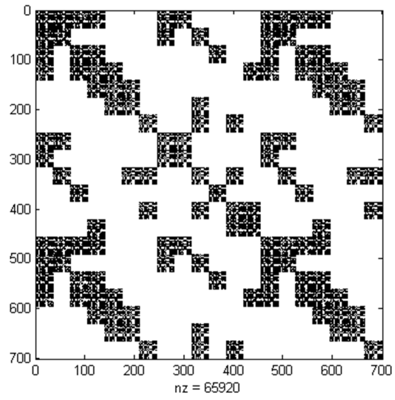
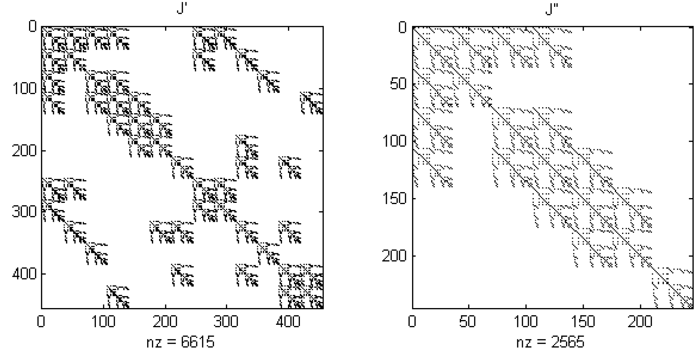
At each iteration, $f_{P_i}^n$ $f_{Q_i}^n$ in $J$ need to be evaluated at N quadrature nodes, and their sum needs to be calculated for each element in $J$. Therefore, the Newton’s iteration of SG is very expensive. Even if the power system is small and $J$ is sparse, it can still be unsolvable. For example, Figure 1 shows the structure of $J$ in the IEEE 14-bus test system; if $D=4$, $\mathrm{P}=3$, $\mathrm{K}=35$, there will be 124 sub-blocks and 65,920 non-zeros in $J,$ and $(65920\times \mathrm{N}\times \mathrm{L})$ calculation times are needed to renew $J$ if L iterations are used.

Utilizing the P-Q decoupled characteristic in power flow calculation, this paper forms constant Jacobian matrices $J^{\prime }$ and $J^{″}$ to avoid the regeneration of Jacobian, the calculation speed will be significantly improved. $B^{\prime }$, $B^{″}$ are the constant Jacobian matrices in the traditional P-Q fast decoupled load flow method [27], which only contains network admittances:

$$\frac{\partial f_{P_i}}{\partial {\mathsf{\theta }}_j}\approx B^{\prime }(i,j);\frac{\partial f_{P_i}}{\partial V_j}\approx 0;\frac{\partial f_{Q_i}}{\partial V_j}\approx B^{″}(i,j);\frac{\partial f_{Q_i}}{\partial {\mathsf{\theta }}_j}\approx 0$$

(24)

Applying Equation (24) in the derivation of $J$ above, $J$ changed into two constant matrices $J^{\prime }\in R^{N_2\times N_2}$, $J^{″}\in R^{N_1\times N_1}$ which only need to be calculated once (see the Appendix). Figure 2 shows the structure of matrices $J^{\prime }$ and $J^{″}$ after the matrix $J$ in Figure 1 is decoupled; there will be 6615 and 2565 nonzeros in $J^{\prime }$ and $J^{″}$, and $(9180\times \mathrm{N})$ calculation times are needed, which is far less than before.

For ease of expression, N constant matrices $[{\Phi }_1,\dots ,{\Phi }_N]$ are constructed at N quadrature nodes:

$${\Phi }_n=W^n\mathsf{\psi }{(n,:)}^T\mathsf{\psi }(n,:)\in R^{\mathrm{K}\times \mathrm{K}},n\in [1,\mathrm{N}]$$

(25)

Thus $J^{\prime }$ and $J^{″}$ can be expressed as:

$$\{\begin{array}{c}{J}^{\prime }=B^{\prime }\otimes {\displaystyle {\sum }_{n=1}^N{\Phi }_n}\\ J^{″}=B^{″}\otimes {\displaystyle {\sum }_{n=1}^N{\Phi }_n}\end{array}$$

(26)

$\underset{˜}{\widehat{\mathsf{\theta }}}$, $\underset{˜}{\widehat{V}}$ can be computed directly by Newton iteration method:

$$\mathrm{Solve}:\{\begin{array}{c}\left[\frac{\Delta {\underset{˜}{G}}_P}{\underset{˜}{\widehat{\mathsf{\theta }}}}\right]=J^{\prime }\left[\Delta \underset{˜}{\widehat{\mathsf{\theta }}}\right]\\ \left[\frac{\Delta {\underset{˜}{G}}_Q}{\underset{˜}{\widehat{V}}}\right]=J^{″}\left[\Delta \underset{˜}{\widehat{V}}\right]\end{array}$$

(27)

$$\mathrm{Update}:\{\begin{array}{c}{\underset{˜}{\widehat{\mathsf{\theta }}}}^{r+1}={\underset{˜}{\widehat{\mathsf{\theta }}}}^r+\Delta {\underset{˜}{\widehat{\mathsf{\theta }}}}^r\\ {\underset{˜}{\widehat{V}}}^{r+1}={\underset{˜}{\widehat{V}}}^r+\Delta {\underset{˜}{\widehat{V}}}^r\end{array}$$

(28)

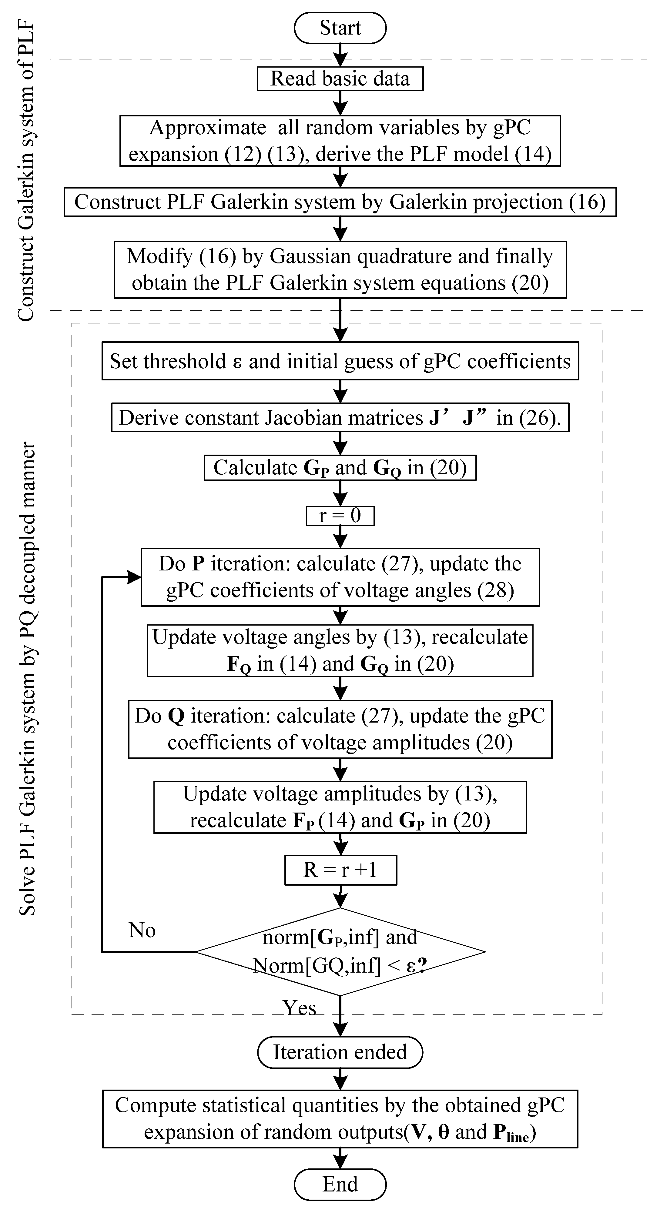
The proposed PLF method (referred to as SG-PLF method) only needs to compute deterministic PLF Galerkin system Equation (20) and construct constant Jacobian matrices Equation (26) at limited quadrature nodes, then solve Equation (20) by the Newton iteration method only once to reach high accuracy. The flow chart of the SG-PLF method is depicted by Figure 3, which consists of two parts.

Firstly, based on the system basic data and PDF of input random variables, we form the PLF model Equation (14) based on gPC expansion of random variables and transform it into Equation (16) by Galerkin projection, then further approximate Equation (16) by Gaussian quadrature, and finally obtain the PLF Galerkin system Equation (20). Secondly, we solve the Galerkin system for coefficients $\widehat{\mathsf{\theta }},\widehat{V}$ directly by a Newton iteration method, and the gPC expansion of random output variables can be derived easily.

4. Comparison with other PLF Methods

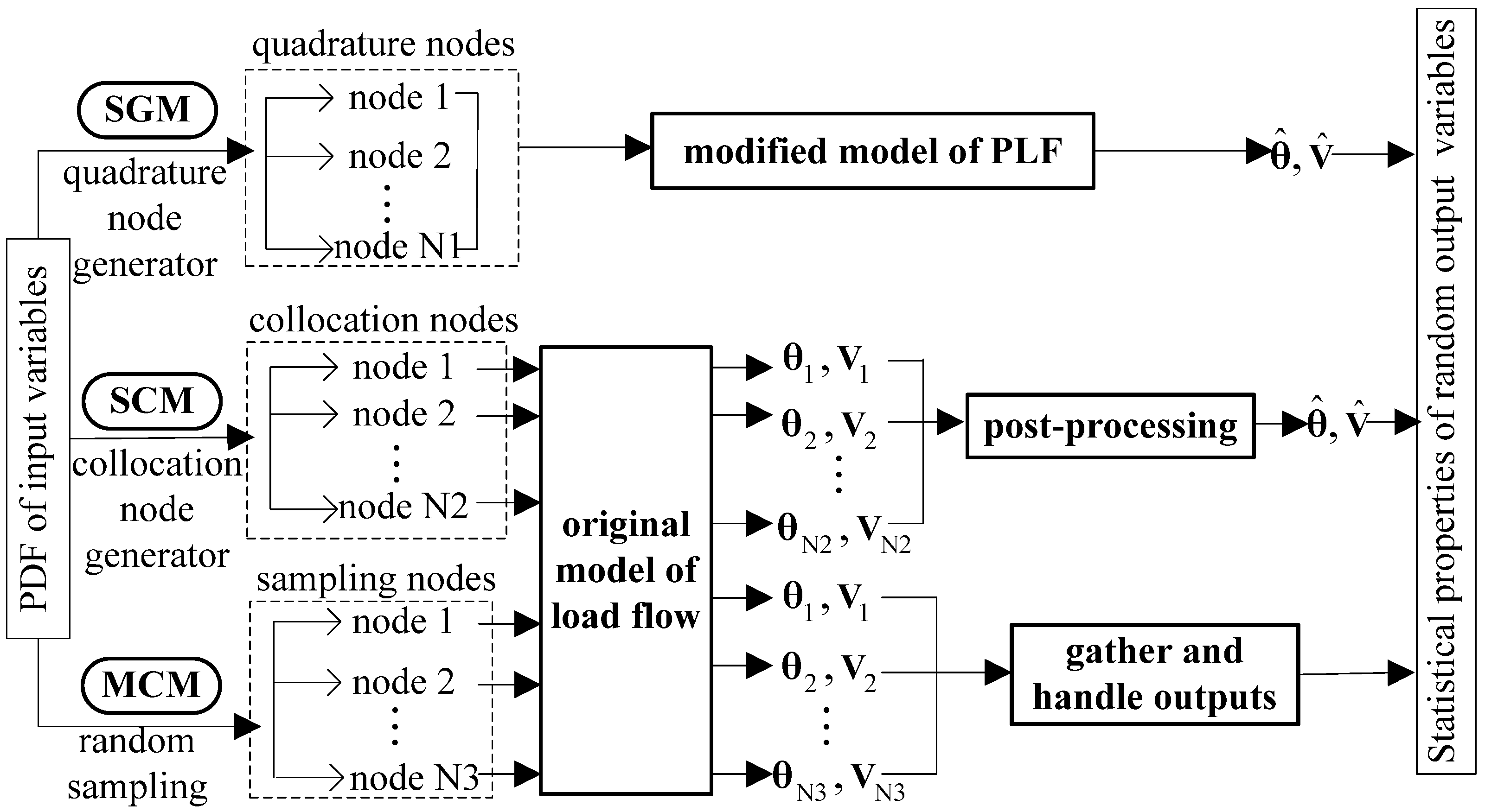
This section compares the calculation procedures of MCM, SC method (SCM) and the proposed modified SG method (SGM); see Figure 4.

MCM and SCM are both non-intrusive methods, they both start from the original load flow Equation (11) without using gPC approximation a priori, and compute the deterministic solutions at a set of nodes. The main difference of MCM and SCM lies in how to select the nodes. MCM draws sampling nodes randomly according to the PDF of $\mathsf{\xi }$ and is uncertainty-dimension independent; the MCM may be the only choice when the number of random variables to be dealt with is too high (in ultra-high-dimensional problem). However, SCM constructs collocation nodes with a nodes generator which uses cubature rules such as tensor product, nested grid or sparse grid techniques. After repeatedly simulating deterministic load flow equations, MCM provides the statistical information by gathering and handling the resulting outputs, whereas SCM reconstructs the gPC coefficients in a post-processing step such as numerical integration. For example, SCM constructs ${\mathrm{N}}_2$ collocation nodes $[{\mathsf{\xi }}^1,\dots ,{\mathsf{\xi }}^{N_2}]$ and weights $[W^1,\dots ,W^{N_2}]$ of random output variable $S(\mathsf{\xi })$ (in Equation (8)), and then the gPC coefficients can be computed by:

$${\widehat{s}}_k\approx \langle S(\mathsf{\xi }),{\mathsf{\psi }}_k(\mathsf{\xi })\rangle \approx {\displaystyle {\sum }_{n=1}^{{\mathrm{N}}_2}{W}^n{\mathsf{\psi }}_k({\mathsf{\xi }}^n)}S({\mathsf{\xi }}^n)$$

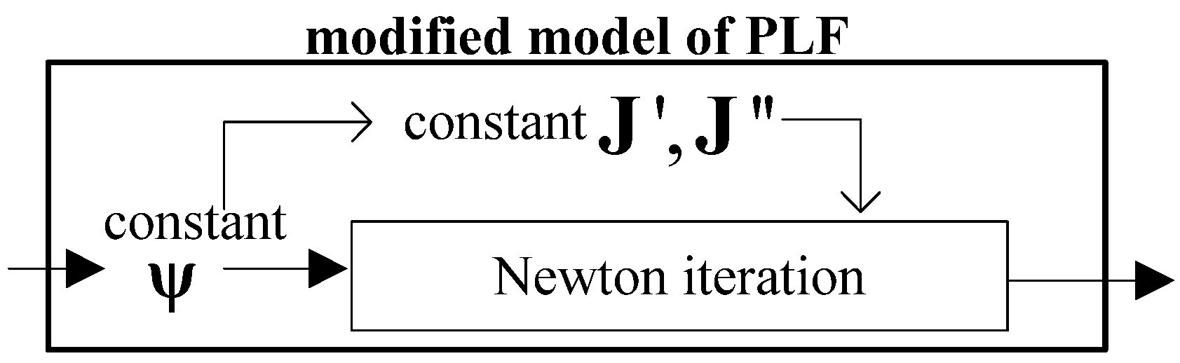
The SGM is an intrusive method as it directly computes the gPC coefficients by simulating a larger-size coupled PLF only once. With gPC approximation, it starts from the residual function Equation (14). The proposed SG-PLF method constructs nodes by sparse grid technique and modified the SGM by utilizing the P-Q decoupling properties of power system, which can avoid the heavy computation burden of forming Jacobian matrix in each iteration. Figure 5 shows a detailed illustration of the modified calculation model of the proposed SG-PLF method.

If the original load flow Equation (11) are solved by P-Q fast decouple method, and the time cost of solving is $t_{or}.$ then the total time cost by MCM is $(t_{or}\times {\mathrm{N}}_3),$ where ${\mathrm{N}}_3$ is much larger than ${\mathrm{N}}_1$ and ${\mathrm{N}}_2.$ If the node generators in SCM and SGM are both using the sparse grid technique, where ${\mathrm{N}}_1={\mathrm{N}}_2=\mathrm{N},$ set the time for constructing nodes is $t_{no}$ and the time cost of post-processing is $t_{po}.$ Thus, the total time cost of SCM is $(t_{no}+t_{or}\times N+t_{po}).$ In SGM, the times needed for constructing constant Jacobian matrices are $t_{cj}$ and for solving the modified model are $t_{mo},$ so the total time required for SGM is $(t_{no}+t_{mo}+t_{cj})$.

The dimension of modified PLF model in SGM is $\mathrm{K}\times \mathrm{N}$ times the size of the original PLF model, and the equations need to be solved in SCM is $\mathrm{N}$ times the size of the original PLF model. $t_{cj}$ can be ignored, and $t_{mo}$ is slightly larger than $t_{or}\times \mathrm{N}+t_{po}$, so there are no significant difference between the total computational time of SCM and SGM , this can be verified in the following case study.

In conclusion, on the one hand, since ${\mathrm{N}}_3$ is much larger than ${\mathrm{N}}_1$ and ${\mathrm{N}}_2$, MCM needs numerous deterministic load flow calculations to obtain accurate results, the SG-PLF method has a distinct speed advantage over MCM. On the other hand, SCM only requires no errors at each collocation node and will introduce aliasing errors caused by the introduction of the nodal sets, whereas the SG-PLF method ensures that the residue of the PLF Equation (14) is orthogonal to the linear space spanned by the gPC basis functions, as in Equation (16). In this sense, the accuracy of SGM is optimal.

Therefore, the proposed SG-PLF method has accuracy advantage over the non-intrusive SCM and speed advantage over the MCM.

5. Case study

5.1. Verification Index

In order to evaluate the computational accuracy and efficiency of SG-PLF method, a series of PLF studies are carried out on the modified IEEE14-bus and IEEE 118-bus test systems. The base case data of these two test systems are available in [28]. Two types of input random variables are considered in this case study, load and wind power included. Relative error $\mathsf{\epsilon }$ (RE) [5] and average root mean square (ARMS) [12] error $\mathsf{\tau }$ are computed using the MCM results of 30,000 trials as reference. RE is defined as:

$${\mathsf{\epsilon }}_s^x=\left|(s_G^x-s_M^x)/s_M^x\right|\times 100\%$$

(29)

The ARMS is defined as:

$${\mathsf{\tau }}^x=\sqrt{{{\displaystyle {\sum }_{t=1}^T(X_{Gt}^x-X_{Mt}^x)}}^2}/T$$

(30)

where $x$ refers to the type of random output variables ($V$, $\mathsf{\theta }$ and $P_{line}$ etc.), $s$ may refer to the mean $\mathsf{\mu }$ and standard deviation $\mathsf{\sigma }.$ $s_M^x$ denotes the result calculated by MCM and is taken as the reference value, $s_G^x$ is the result obtained by SG-PLF method. ${\mathsf{\epsilon }}_{s,\mathrm{mean}}^x$ and ${\mathsf{\epsilon }}_{s,\max }^x$ are the average and maximum values of ${\mathsf{\epsilon }}_s^x.$ Choosing T sampling nodes of variable $\mathsf{\xi }$ arbitrarily: $[{\mathsf{\xi }}^1,\dots ,{\mathsf{\xi }}^T]$, $X_{Gt}$ and $X_{Mt}$ are the outputs of the SG-PLF method and MCM at the $t\mathrm{th}$ node ${\mathsf{\xi }}^t(t\in [1,T])$.

5.2. IEEE 14-Bus Test System

The case considered in this section is the IEEE 14-bus test system which is modified to include wind generation. The uncertainties of forecasted loads are modeled as normal distribution with $\mathsf{\sigma }$ 5% to $\mathsf{\mu }$, whose means equal the base case data. The load correlation matrix between bus 4 and bus 5 is ${\mathsf{\rho }}_l$. Two wind farms are located at bus 13 and bus 14, and their wind speed correlation matrix is ${\mathsf{\rho }}_v$:

$${\mathsf{\rho }}_l=\left[\begin{array}{cc}1& 0.5\\ 0.5& 1\end{array}\right];{\mathsf{\rho }}_v=\left[\begin{array}{cc}1& 0.6\\ 0.6& 1\end{array}\right]$$

(31)

The wind power is mainly affected by wind speed distribution, power curve and control strategy of wind turbine generator. The wind speed is assumed to follow the Weibull distribution with scale parameter as 10.7 and shape parameter as 3.97. The wind speed is transformed into wind power according to the power curve of wind turbine generator $P_{\mathrm{W}}(v)$ [3]: the cut-in, rated and cut-off speeds are $v_{ci}=4 \mathrm{m}/\mathrm{s},v_r=15 \mathrm{m}/\mathrm{s},v_{co}=25 \mathrm{m}/\mathrm{s}$ respectively, and the rated power $P_{\mathrm{Wr}}$ is 0.7 p.u. The wind turbine generator is controlled by constant power factor strategy.

$$P_{\mathrm{W}}(v)=\{\begin{array}{c}0,v<v_{ci}\mathrm{or}v>v_{co}\\ P_{Wr}\frac{v^2-v_{ci}^2}{v_r^2-v_{ci}^2},v_{ci}\le v<v_r\\ P_{Wr},v_r\le v\le v_{co}\end{array}$$

(32)

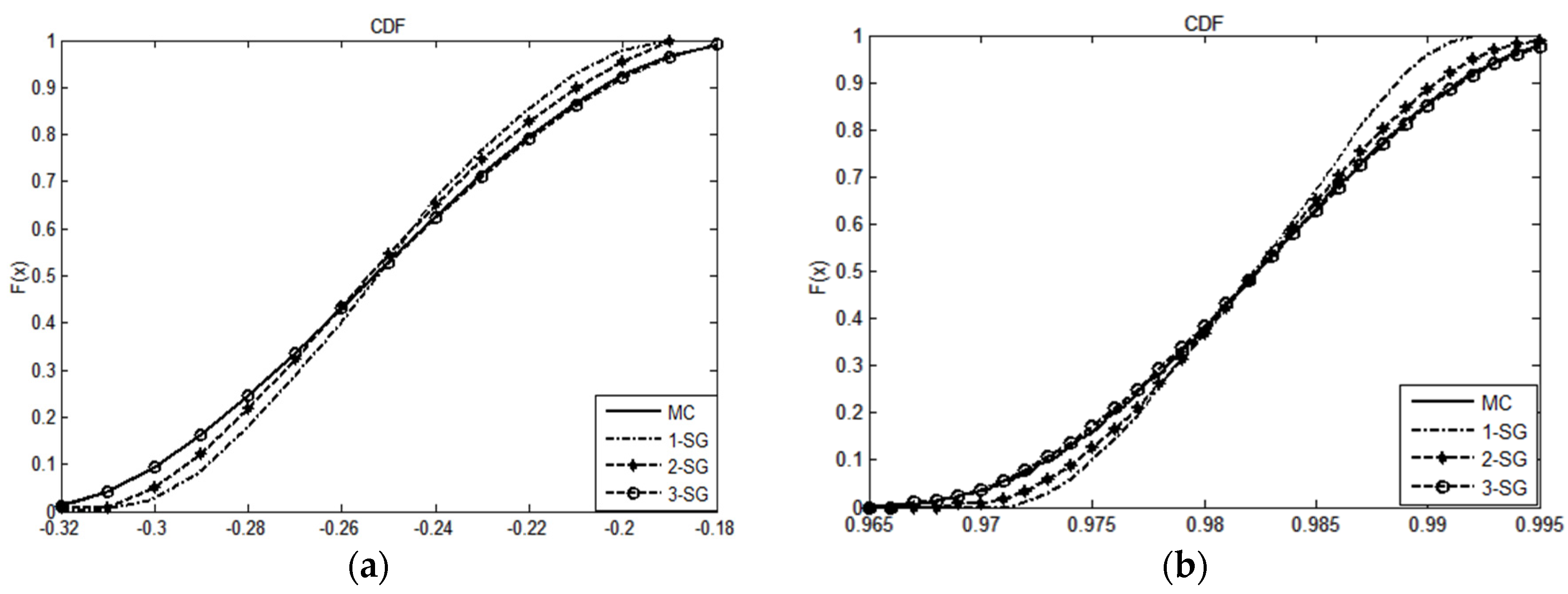
5.2.1. Impact of the gPC Expansion Order

Figure 6 shows the CDFs obtained by SG-PLF method under different gPC expansion order P (defined in Equation (7)). The results shows that the order-3 SG-PLF method provides good fitting to the CDF obtained by MCM, gives an intuitive confirmation that the order-3 SG-PLF method has the ability to well handle over the PLF problem as almost the same accuracy as the MCM.

Furthermore, the resulted ${\mathsf{\epsilon }}_{s,\mathrm{mean}}^{\mathsf{\gamma }}$ and ${\mathsf{\epsilon }}_{s,\max }^{\mathsf{\gamma }}$ under different order P are shown in

Table 2. Mean and maximum of ER of SG-PLF under 1-3 order.

$\mathit{x}$	Order-P	${\mathsf{\epsilon }}_{\mathit{s}\mathbf{mean}}^{\mathit{x}}\mathbf{/}\mathbf{100}\mathbf{\%}$		${\mathsf{\epsilon }}_{\mathit{s}\mathbf{max}}^{\mathit{x}}\mathbf{/}\mathbf{100}\mathbf{\%}$
		s = μ	s = σ	s = μ	s = σ
$V$	1	8.38 × 10−2	6.34	9.16 × 10−2	8.17
	2	2.14 × 10−2	3.88	1.07 × 10−2	8.06
	3	8.69 × 10−4	0.332	1.13 × 10−3	2.32
$\mathsf{\theta }$	1	1.01	7.90	2.50	10.3
	2	0.745	6.02	1.33	8.65
	3	7.78 × 10−2	0.582	0.139	0.920

, which verified the good computing performance of the order-3 SG-PLF method.

Therefore, the gPC expansion order P can affect the calculation performance of the proposed method: when P is too low, the gPC expansion approximation Equation (8) will induce large truncation error; when P is too high, the number of quadrature nodes N will increase significantly, so it will lead to increasing of calculation but no progress in computation accuracy, because all the high order gPC coefficients in gPC expansion approximation Equation (8) will be zeros. In this paper, the expansion order is chosen by numerical experiments, but direct methods to determine the order are to be further studied in our future work.

To further investigate the calculation efficiency of using the SGM to solve PLF, the calculation time and nodes number N of SGM, SCM and MCM are compared in

Table 3. Computation time comparison.

Method	Expansion Order P						MCM
	1		2		3
	SCM	SGM	SCM	SGM	SCM	SGM
Time/s	0.011	0.011	0.053	0.099	0.188	0.298	13.326
Nodes (N)	9		41		145		30,000

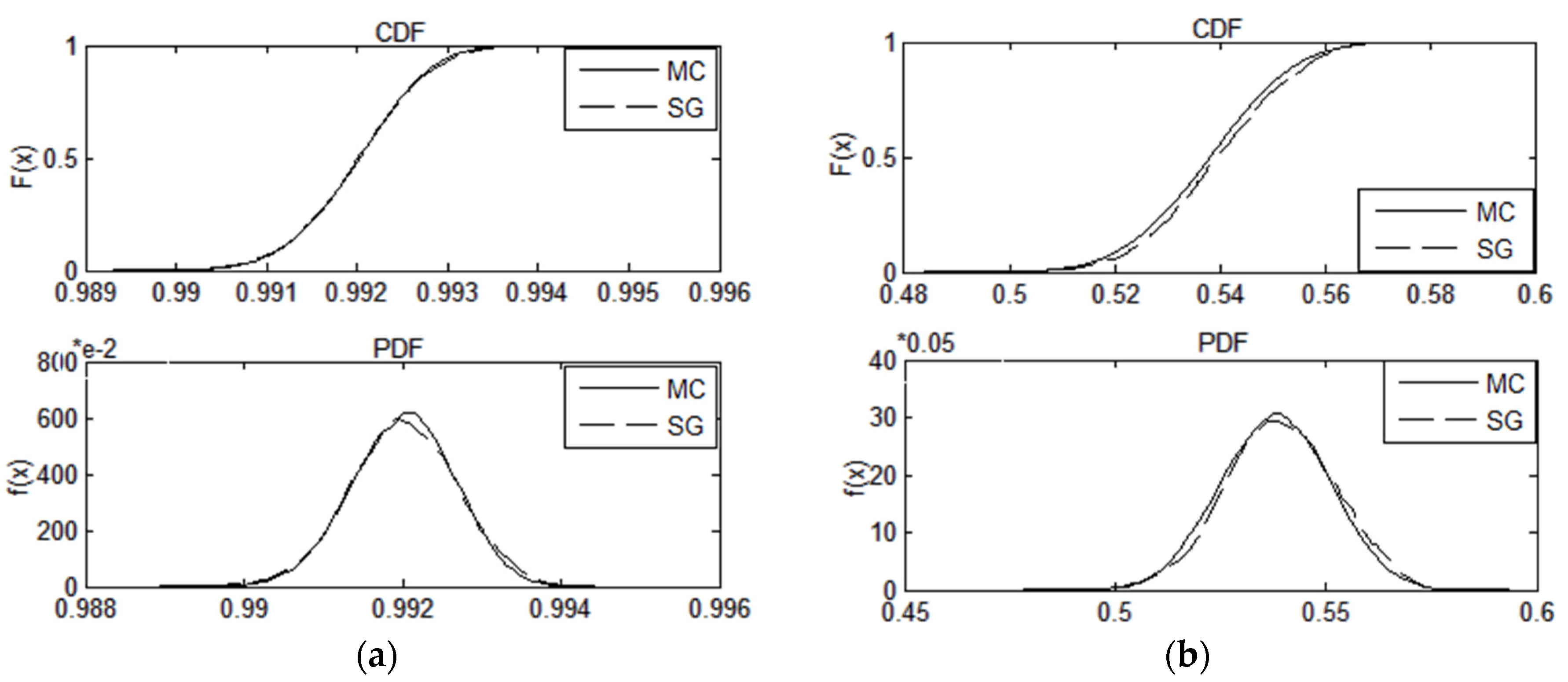
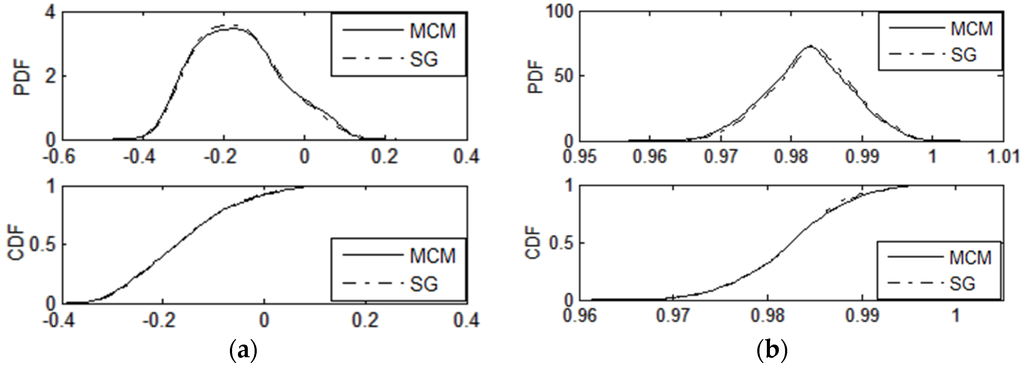
, in which, the gPC-based SCM and SGM both construct the nodes according to the sparse grid technique, and the time cost with different P are compared. Figure 7 shows the PDFs and CDFs of the buses whose power injection have large fluctuations, and the results corresponding to the order-3 SG-PLF method are almost not visible because they coincide with those of MCM.

From the results above, the order-3 SG-PLF method can maintain high accuracy with feasible computation expense. This conclusion is further confirmed by comparing the ARMS results of the order-3 SG-PLF method in

Table 4. Mean and maximum of ARMS of order-3 SG-PLF method.

ARMS	${\mathsf{\tau }}^{\mathsf{\theta }}\mathbf{/}\mathbf{100}\mathbf{\%}$	${\mathsf{\tau }}^{\mathit{V}}\mathbf{/}\mathbf{100}\mathbf{\%}$
Mean	1.60 × 10−4	1.24 × 10−5
Maximum	3.13 × 10−4	2.14 × 10−5

. Thus in the following study, the order-3 SG-PLF method is used for PLF investigation and verification.

Take the frequency table of $V_4$ as an example, set the results of MCM as the reference, and further compare the calculation accuracy of order-3 SCM and order-3 SGM, shown in

Table 5. The frequency table of different methods.

Distribution Interval of ${\mathit{V}}_{\mathbf{4}}$	Probability/100%
	MCM	SGM	SCM
[1.0122,1.0146)	0.96	0.96	0.95
[1.0146,1.0169)	3.76	3.64	3.36
[1.0169,1.0193)	7.68	7.79	8.17
[1.0193,1.0216)	12.08	11.88	11.35
[1.0216,1.0240)	15.12	15.54	15.69
[1.0240,1.0263)	16.64	16.43	16.16
[1.0263,1.0287)	15.28	15.31	15.52
[1.0287,1.0311)	15.12	15.10	15.03
[1.0311,1.0334)	8.56	8.69	8.97
[[1.0334,1.0358]	5.04	5.01	4.80

:

In this section, the results above show that:

(1) the MCM can achieve the highest accuracy, but it needs the longest calculation time; and

(2) although the computational speed of SGM is slightly slower than SCM, the intrusive SGM has obvious precision advantage than SCM (which is also analyzed in Section 4).

Therefore, through comprehensive consideration of calculation speed and accuracy, the proposed SG-PLF method is the optimal among three methods.

5.2.2. Impact of the Fluctuation of Power Injection

In order to appraise how the variation level of uncertain variable impacts on the calculation performance of the proposed order-3 SG-PLF method,

Table 6. Mean and maximum of RE of order-3 SG-PLF with different load variance.

$\mathit{x}$	Ratio $\mathsf{\sigma }/\mathsf{\mu }$	${\mathsf{\epsilon }}_{\mathit{s}\mathbf{mean}}^{\mathit{x}}\mathbf{/}\mathbf{100}\mathbf{\%}$		${\mathsf{\epsilon }}_{\mathit{s}\mathbf{max}}^{\mathit{x}}\mathbf{/}\mathbf{100}\mathbf{\%}$
		s = μ	s = σ	s = μ	s = σ
$V$	10%	2.76 × 10−3	0.899	1.15 × 10−2	4.44
	20%	2.21 × 10−3	0.618	8.78 × 10−3	4.55
	30%	2.65 × 10−3	0.422	1.37 × 10−2	4.58
	40%	2.83 × 10−3	0.369	1.12 × 10−2	4.23
$\mathsf{\theta }$	10%	0.316	2.48	0.737	3.11
	20%	0.182	2.13	0.265	3.19
	30%	0.264	1.27	0.771	2.55
	40%	0.498	1.75	0.653	1.41

shows the ${\mathsf{\epsilon }}_{s,\mathrm{mean}}^{\mathsf{\gamma }}$ and ${\mathsf{\epsilon }}_{s,\max }^{\mathsf{\gamma }}$ of proposed method under different load fluctuations at bus 4 (set the ratio of $\mathsf{\sigma }$ to $\mathsf{\mu }$ is from 10% to 40%).

From the results, it can be inferred that the variance level of power injection has no discernible effect on the calculation accuracy of the proposed method.

5.2.3. Impact of Wind Speed Correlation

Choose the statistical moments of active line power (mean $\mathsf{\mu }-P_{line}$ and standard deviation $\mathsf{\sigma }-P_{line}$) as the research objects in this section. The uncertain wind powers of two wind farms are directly injected into both the end of lines 13–14, while lines 1–2 have no direct connection to wind power.

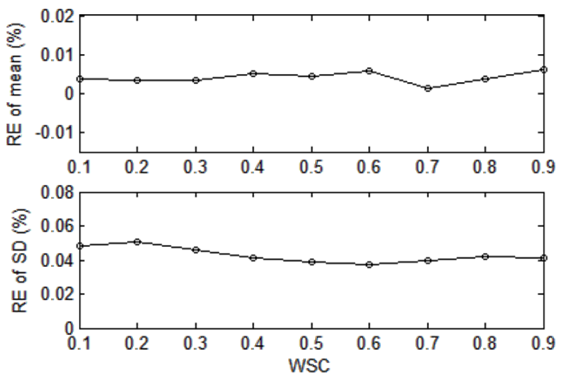
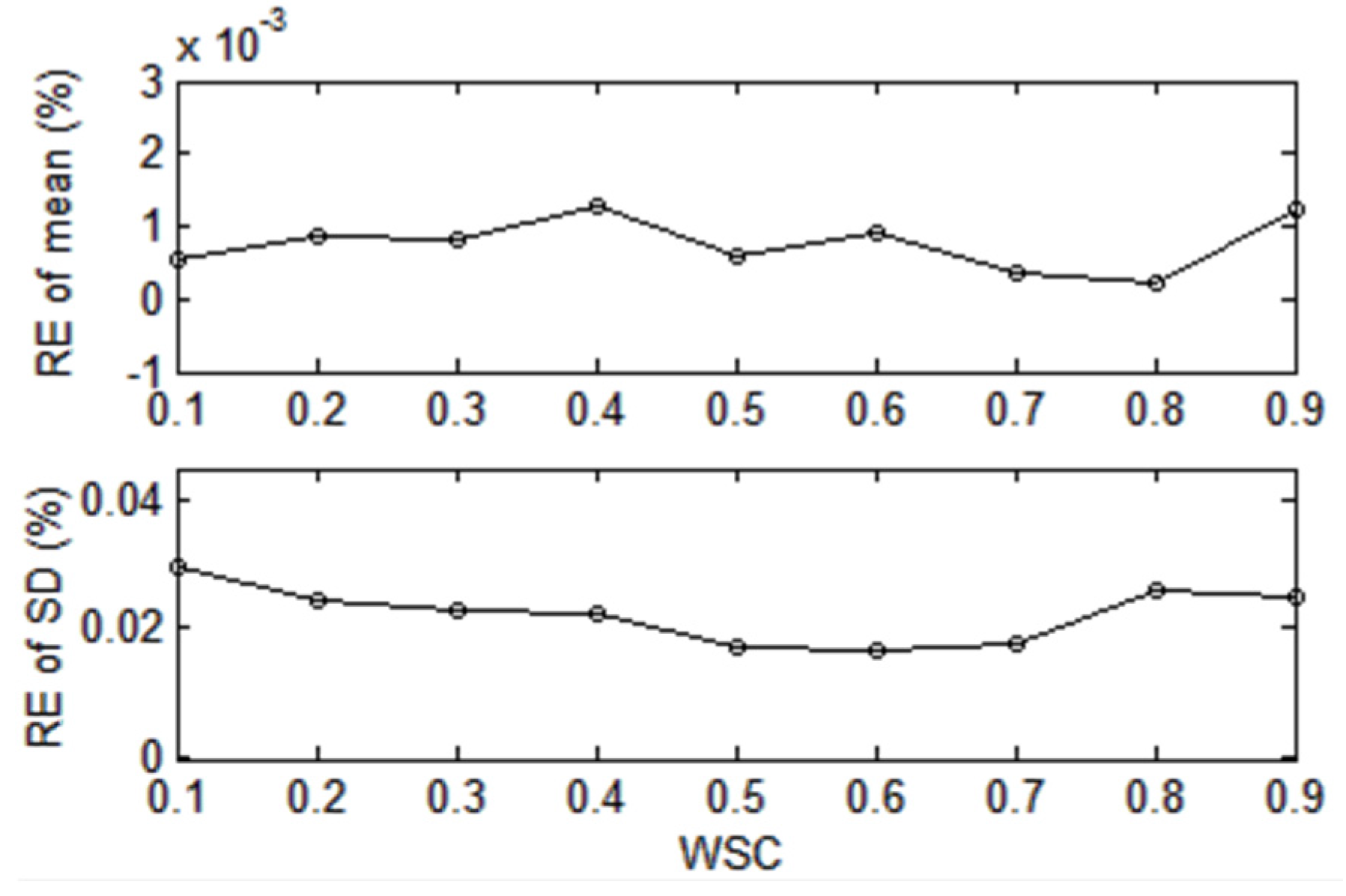
Under different wind speed correlations (WSC) between two wind farms, Figure 8 and Figure 9 present the calculated mean and standard deviation (SD) values of the REs of all buses and illustrate how the calculation accuracy of the proposed 3-order SG-PLF method will change with the WSC growing from 0.1 to 0.9. The results show that WSC has a minor effect on the calculation accuracy of the proposed method. 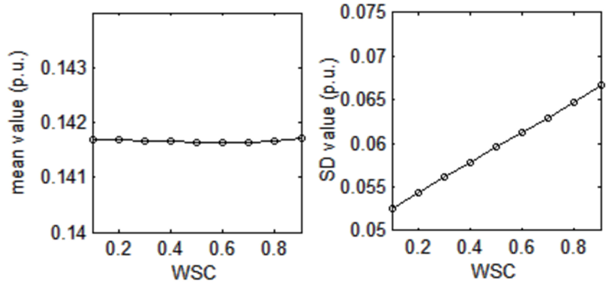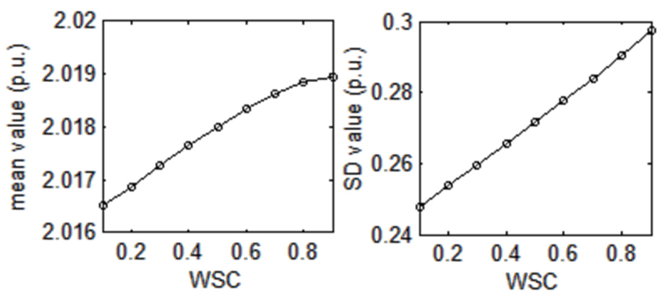Figure 10 and Figure 11 present the values of $\mathsf{\mu }-P_{line}$ and $\mathsf{\sigma }-P_{line}$ with WSC growing from 0.1 to 0.9. Results show that, at different sites, the WSC has different impact on system condition. $\mathsf{\mu }-P_{13-14}$ remains basically unchanged but $\mathsf{\sigma }-P_{13-14}$ is proportional to WSC, while $\mathsf{\mu }-P_{1-2},\mathsf{\sigma }-P_{1-2}$ are all proportional to WSC.

5.3. IEEE 118-Bus Test System

In this section, PLF problem is solved for the IEEE 118-bus test system with the purpose of assessing how an increase in the uncertainty level (dimension and variance of random variables) would affect the performance of proposed method. From bus 24 to bus 27, each bus is connected to a wind farm, the rated power of each wind turbine generator $P_{\mathrm{Wr}}$ is 0.2 p.u. The random active loads at bus 60, bus 78, bus 79 and bus 82 are assumed to follow Gaussian distribution. The variance of the random loads are larger than the previous case, with $\mathsf{\sigma }$ is 10% to $\mathsf{\mu }$. The correlation matrices of wind speeds and loads are in Equation (33). Other parameters of wind farms are consistent with the previous case.

$${\mathsf{\rho }}_v=\left[\begin{array}{cccc}1& 0.88& 0.6& 0.4\\ 0.88& 1& 0.5& 0.6\\ 0.6& 0.5& 1& 0.8\\ 0.4& 0.6& 0.8& 1\end{array}\right];{\mathsf{\rho }}_l=\left[\begin{array}{cccc}1& 0.5& 0.48& 0.6\\ 0.5& 1& 0.48& 0.5\\ 0.48& 0.48& 1& 0.3\\ 0.6& 0.5& 0.3& 1\end{array}\right]$$

(33)

To solve this case, the calculation time of MCM is 16.436 s while the order-3 SG-PLF method only takes 3.306 s. The RE and ARMS results of the proposed method are shown in

Table 7. Mean and maximum ERs and ARMSs of 3-order SG-PLF.

x	${\mathsf{\epsilon }}_{\mathit{s}\mathbf{mean}}^{\mathit{x}}\mathbf{/}\mathbf{100}\mathbf{\%}$		${\mathsf{\epsilon }}_{\mathit{s}\mathbf{max}}^{\mathit{x}}\mathbf{/}\mathbf{100}\mathbf{\%}$		${\mathsf{\tau }}_{\mathbf{mean}}^{\mathit{x}}\mathbf{/}\mathbf{100}\mathbf{\%}$	${\mathsf{\tau }}_{\mathbf{max}}^{\mathit{x}}\mathbf{/}\mathbf{100}\mathbf{\%}$
	μ	σ	μ	σ
$V$	1.74 × 10−3	0.91	8.01 × 10−3	1.56	2.09 × 10−6	3.40 × 10−5
$\mathsf{\theta }$	0.313	2.15	0.962	7.54	1.56 × 10−5	6.11 × 10−5

, where the maximum RE values of $V$ and $\mathsf{\theta }$ appeared at bus 26 and bus 49. Figure 12 shows the resulting CDFs and PDFs of $V_{26}$ and ${\mathsf{\theta }}_{49},$ which proved the calculation accuracy of the proposed order-3 SG-PLF method again. Therefore, when the variance and dimension of uncertain variables rise, the proposed method can maintain high accuracy whilst providing significant computational savings.

Based on all of the previous simulation results, the details of some influencing factors on the performance of the proposed SG-PLF method are summarized in

Table 8. Summary on the factors influencing the performance of the proposed SG-PLF method.

Impacting Factor	Accuracy	Speed
Expansion order (P) $\uparrow$	$\uparrow$	$\downarrow$
Efficiency of node generator $\uparrow$	$\uparrow$	$\uparrow$
Dimension of random inputs $\uparrow$	$\to$	$\downarrow$
Dimension of random outputs $\uparrow$	$\to$	$\downarrow$
Variance of random inputs $\uparrow$	$\to$	$\to$
WSC $\uparrow$	$\to$	$\to$
Size of test system $\uparrow$	$\to$	$\downarrow$

, where $\uparrow$ denotes increase, $\downarrow$ means decrease, $\to$ presents minor impact.

6. Conclusions

An intrusive spectral method was proposed in this paper to solve the PLF problem, and simulations in IEEE 14-bus and 118-bus test systems demonstrate its accuracy, efficiency and practicability. The main characteristics of the proposed method are as follows:

• High accuracy. The accuracy of proposed method mainly depends on the gPC expansion approximation Equation (7); by properly choosing the type of gPC basis function and the expansion order P, the proposed methods can offer the optimal accuracy with the least number of equations among all the gPC-based methods.
• Low computation burden. By fully utilizing the P-Q decoupling properties of load flow, the proposed method formed two constant Jacobian matrices in Newton’s iterations, which reduces the computation cost significantly.
• Comprehensibility of the results. The gPC expansion can efficiently handle various random variables and form a functional relationship between the system random inputs and outputs, which is also known as the uncertainty propagation in UQ theory. Thus it can efficiently illustrate the effect of the random inputs on the outputs in PLF problem.

Since the future operating conditions of power system involve more uncertainty due to the growing penetration of distributed generation and renewable energy sources, the proposed method may be increasingly desirable. We believe that it would encourage more interest in UQ research for power systems, with more sophisticated uncertainties and less expenditures of calculation time and resources.

References

- Lin, G.; Engel, D.W.; Esliner, P.W. Survey and Evaluate Uncertainty Quantification Methodologies. PNNL-20914 Rep. Richland. 2012. Available online: http://web.stanford.edu/group/uq/events/UQLS_stanford/Iaccarino.pdf (accessed on 1 March 2016).
- Borkowska, B. Probabilistic load flow. IEEE Trans. Power Appl. Syst. 1974, PAS-93, 752–759. [Google Scholar] [CrossRef]
- Cai, D.F.; Shi, D.Y.; Chen, J. Probabilistic load flow computation with polynomial normal transformation and Latin hypercube sampling. Gener. Transm. Distrib. 2013, 7, 474–482. [Google Scholar] [CrossRef]
- Cui, T.; Franchetti, F. A Quasi-Monte Carlo Approach for Radial Distribution System Probabilistic Load Flow. In Proceeding of the Innovative Smart Grid Technologies (ISGT), Washington, DC, USA, 24–27 February 2013; pp. 1–6.
- Morales, M.J.; Pérez-Ruiz, J. Point Estimate Schemes to Solve the Probabilistic Power Flow. IEEE Trans. Power Syst. 2007, 22, 1594–1601. [Google Scholar] [CrossRef]
- Dopazo, J.F.; Klitin, O.A.; Sasson, M.A. Stochastic load flows. IEEE Trans. Power Appl. Syst. 1975, 94, 752–759. [Google Scholar] [CrossRef]
- Soleimanpour, N.; Mohammadi, M. Probabilistic load flow by using nonparametric density estimators. IEEE Trans. Power Syst. 2013, 28, 3747–3755. [Google Scholar] [CrossRef]
- Morteza, A.; Mahmud, F. Probabilistic Load Flow in Correlated Uncertain Environment Using Unscented Transformation. IEEE Trans. Power Syst. 2012, 27, 2233–2241. [Google Scholar]
- Kolba, D.; Parks, W. A prime factor FFT algorithm using high-speed convolution. IEEE Trans. Acoust. Speech Signal 1977, 25, 281–294. [Google Scholar] [CrossRef]
- Zhang, P.; Lee, S.T. Probabilistic load flow computation using the method of combined cumulants and Gram-Charlier expansion. IEEE Trans. Power Syst. 2004, 19, 676–682. [Google Scholar] [CrossRef]
- Fan, M.; Vittal, V. Probabilistic Power Flow Studies for Transmission Systems with Photovoltaic Generation Using Cumulants, IEEE Trans. Power Syst. 2012, 27, 2251–2261. [Google Scholar] [CrossRef]
- Usaola, J. Probabilistic load flow with correlated wind power injections. Electr. Power Syst. Res. 2010, 80, 528–536. [Google Scholar] [CrossRef]
- Ruiz-Rodriguez, F.; Hernandez, J.; Jurado, F. Harmonic modelling of PV systems for probabilistic harmonic load flow studies. Int. J. Circuit Theory Appl. 2015, 43, 1541–1565. [Google Scholar] [CrossRef]
- Alireza, S.; Mehdi, E. A possibilistic-probabilistic tool for evaluating the impact of stochastic renewable and controllable power generation on energy losses in distribution networks-a case study. Renew. Sustain. Energy 2011, 15, 794–800. [Google Scholar]
- Wiener, N. The homogeneous chaos. Am. J. Math. 1938, 60, 897–936. [Google Scholar] [CrossRef]
- Xiu, D. Numerical Methods for Stochastic Computations: A Spectral Method Approach; Princeton University Press: Princeton, NJ, USA, 2010. [Google Scholar]
- Maitre, L.; Knio, O.; Omar, M. Spectral Methods for Uncertainty Quantification; Springer Netherlands: Dordrecht, The Netherlands, 2010. [Google Scholar]
- Pulch, R. Stochastic Collocation and Stochastic Galerkin Methods for Linear Differential Algebraic Equations. Available online: http://www.imacm.uni-wuppertal.de/fileadmin/imacm/preprints/2012/imacm_12_31.pdf (accessed on 1 March 2016).
- Xiu, D.; Hesthaven, J.S. High-order collocation methods for differential equations with random inputs. SIAM J. Sci. Comput. 2005, 27, 1118–1139. [Google Scholar] [CrossRef]
- Zhang, Z.; El-Moselhy, T.A.; Elfadel, I.M.; Daniel, L. Stochastic testing method for transistor-level uncertainty quantification based on generalized polynomial chaos. IEEE Trans. Comput. Aided Des. Integr. Circuits Syst. 2013, 32, 1533–1545. [Google Scholar] [CrossRef]
- Tang, J.J.; Ni, F.; Ponci, F.; Monti, A. Dimension-adaptive sparse grid interpolation for uncertainty quantification in modern power systems: Probabilistic power flow. IEEE Trans. Power Syst. 2015, 31, 907–919. [Google Scholar] [CrossRef]
- Li, Y.; Li, W.Y.; Yan, W.; Yu, J.; Zhao, X. Probabilistic Optimal Power Flow Considering Correlations of Wind Speeds Following Different Distributions. IEEE Trans Power Syst. 2014, 29, 1847–1854. [Google Scholar] [CrossRef]
- Aien, M.; Firuzabad, M.F. Probabilistic optimal power flow in correlated hybrid Wind–Photovoltaic power systems. IEEE Trans. Power Syst. 2014, 5, 130–138. [Google Scholar] [CrossRef]
- Smolyak, S.A. Quadrature and interpolation formulas for tensor products of certain classes of functions. Soviet Math. 1963, 4, 240–243. [Google Scholar]
- Gerstner, T.; Griebel, M. Numerical integration using sparse grids. Numer. Algorithms. 1998, 18, 209–232. [Google Scholar] [CrossRef]
- MATLAB Source Codes. Available online: http://people.sc.fsu.edu/~jburkardt/m_src/m_src.html (accessed on 15 October 2011).
- Stott, B.; Alsac, O. Fast decoupled load flow. IEEE Trans. Power App. Syst. 1974, PAS-93, 859–869. [Google Scholar] [CrossRef]
- Power Systems Test Case Archive. Available online: http://www.ee.washington.edu/research/pstca (accessed on 1 March 2016).
Figure 1.
Structure of Jacobian matrix for an IEEE 14-bus test system with D = 4 before decoupling.
Figure 2.
Structure of Jacobian matrix for IEEE 14-bus test system with D = 4 after decoupling.
Figure 3.
Flow chart of the proposed SG-PLF method.
Figure 4.
Calculation procedure of PLF by SGM, SCM and MCM.
Figure 5.
Modified calculation model of SG-PLF.
Figure 6.
CDFs of and under 1–3 order in IEEE-14 system: (a) ; (b) .
Figure 7.
PDFs and CDFs of θ, V at the bus which has large fluctuation: (a) θ14(rad); (b) V4(p.u.).
Figure 8.
of 3-order SG-PLF method under different WSC.
Figure 9.
Figure 10.
of 3-order SG-PLF under different WSC.
Figure 11.
Figure 12.
CDFs and PDFs of and in IEEE-118 system: (a) (p.u.); (b) (rad).