
Improved Sensorless Control of Interior Permanent Magnet Sensorless Motors Using an Active Damping Control Strategy


Abstract
:1. Introduction
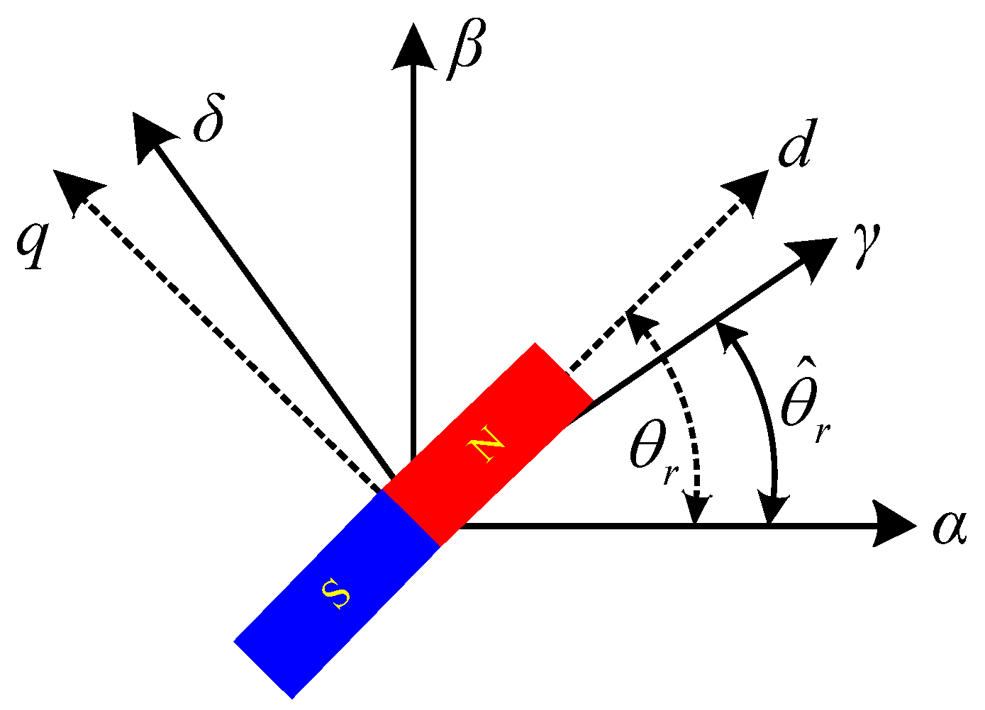
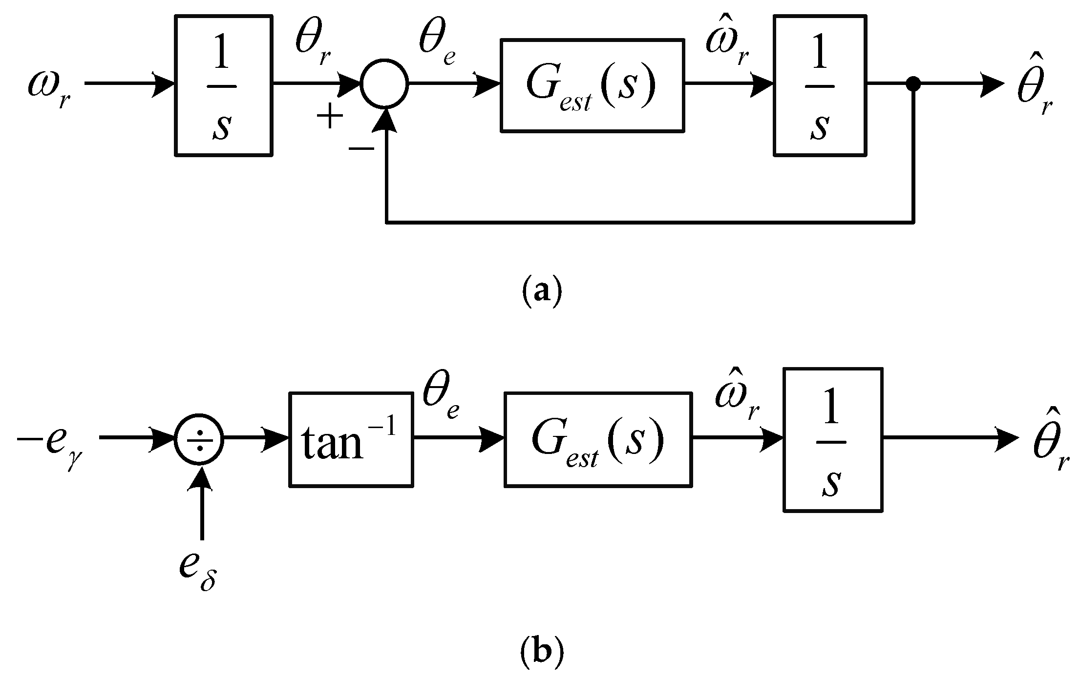
2. Extended EMF Based Sensorless Control of IPM Motor
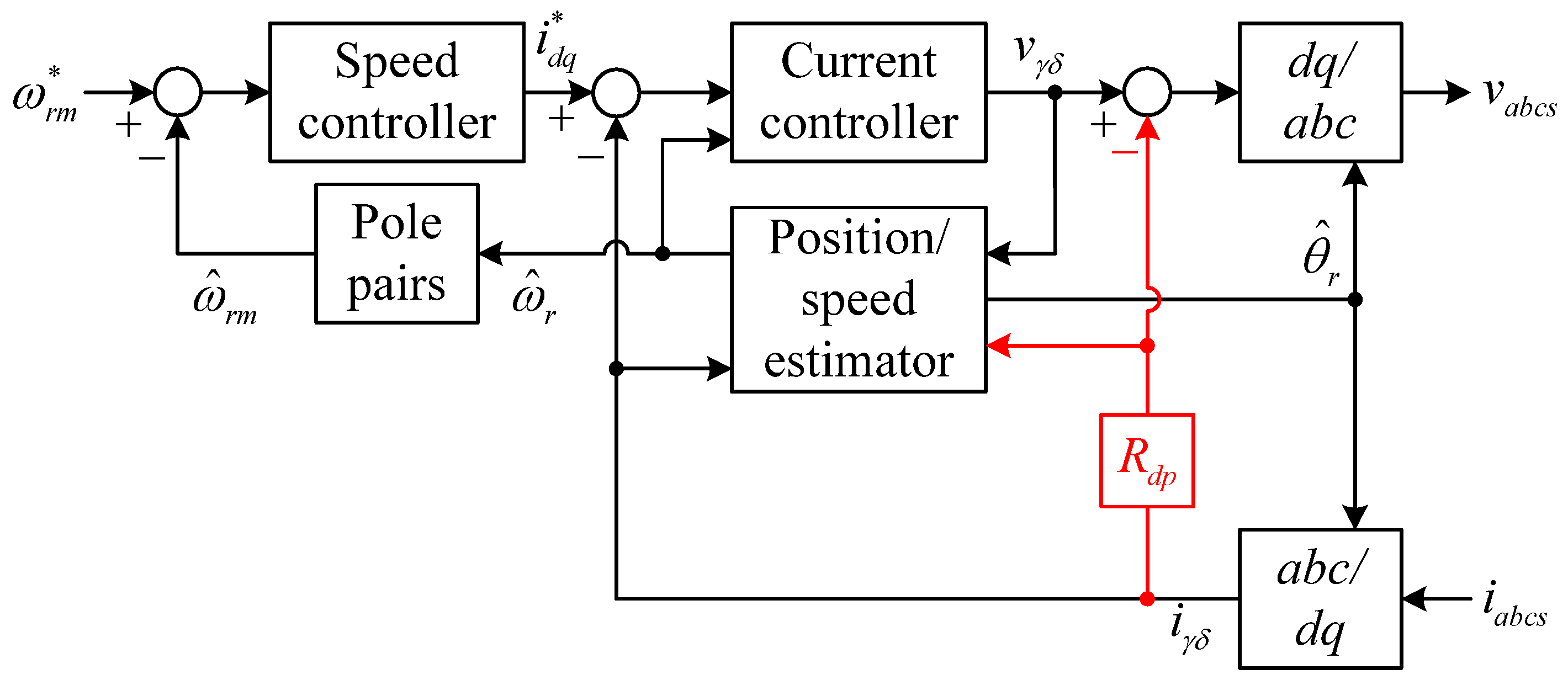
3. Sensorless Control with Active Damping Control Strategy
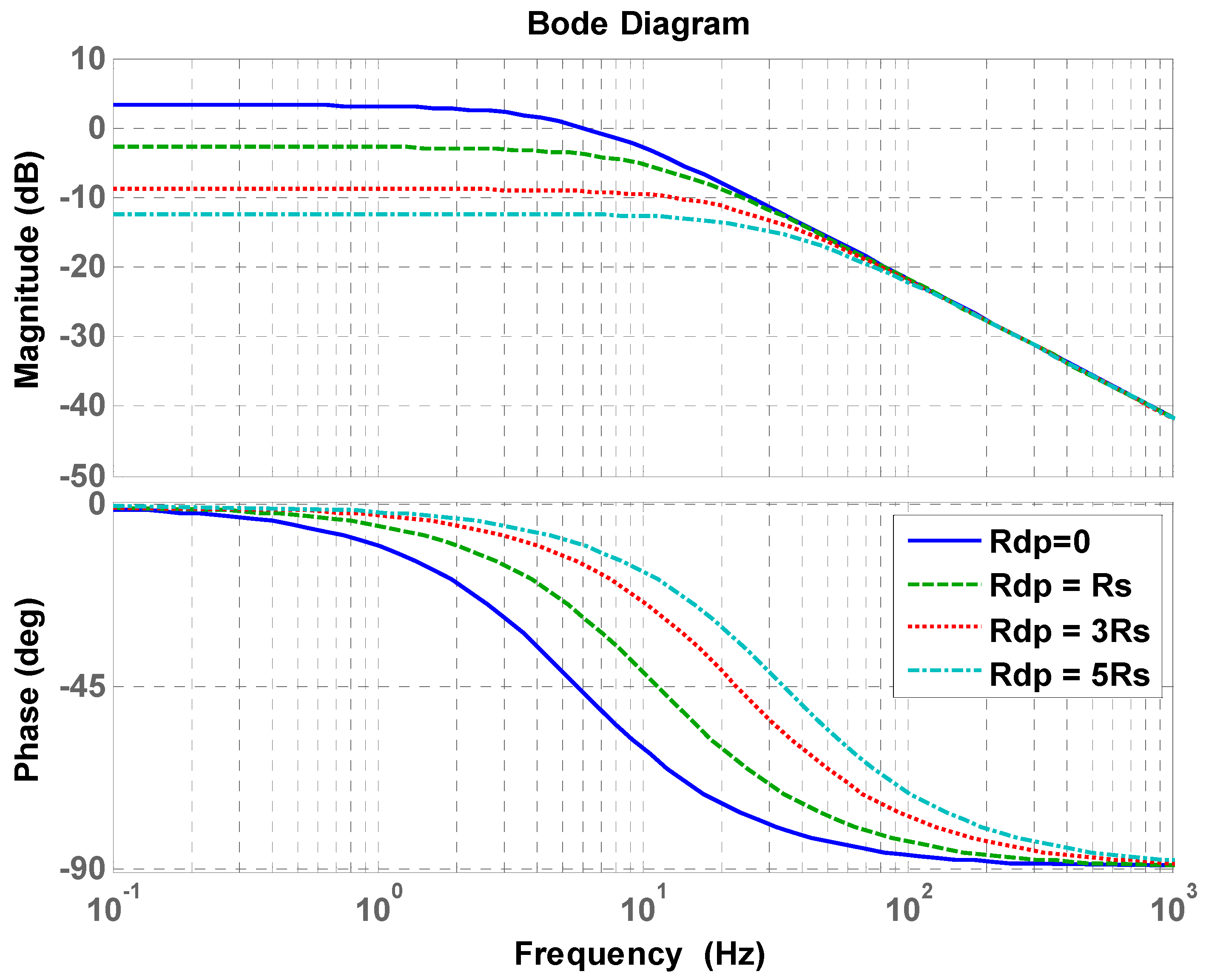
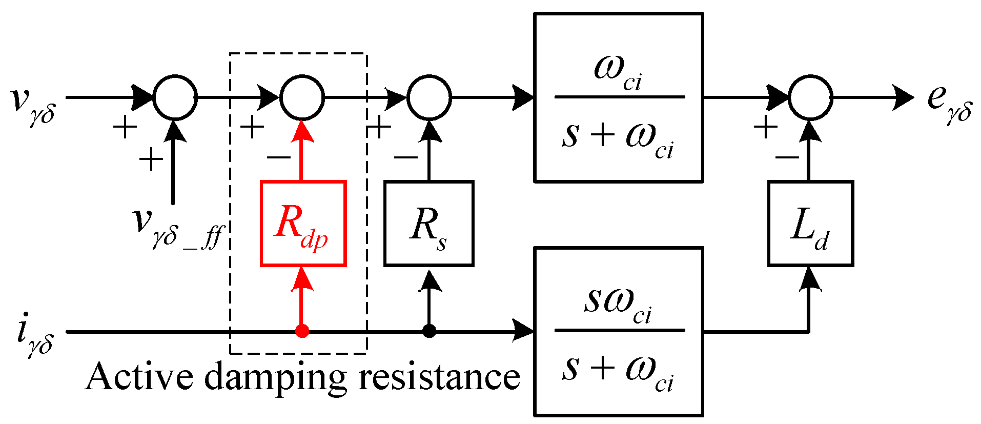
3.1. Back EMF Estimation with Active Damping Control
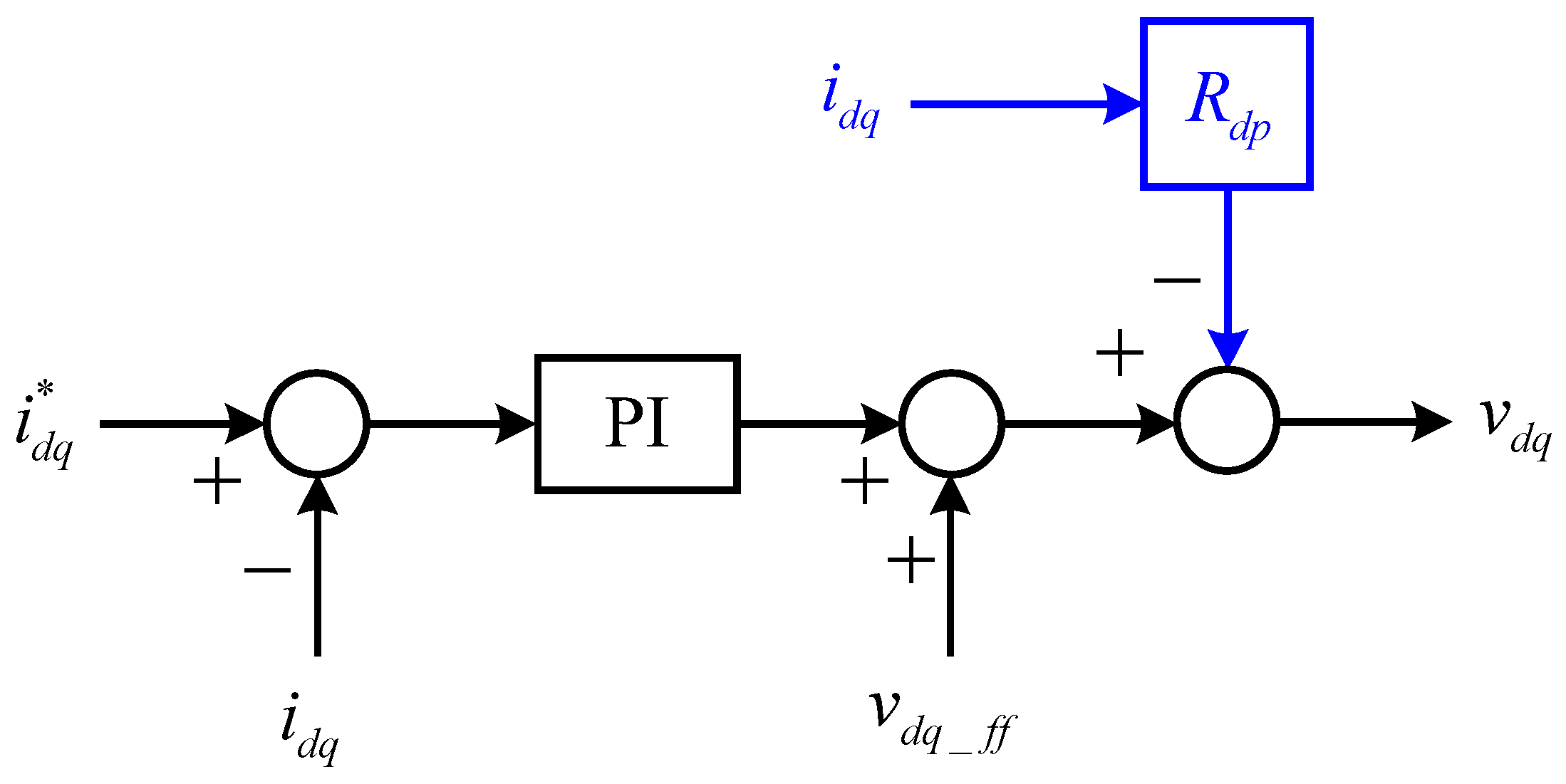
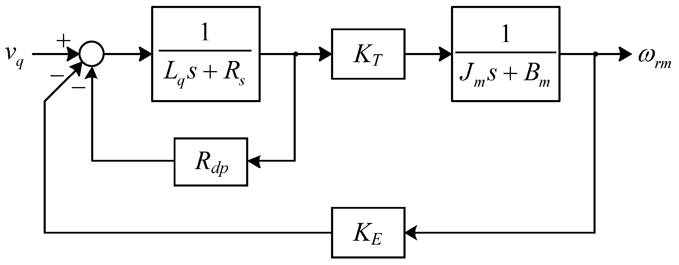
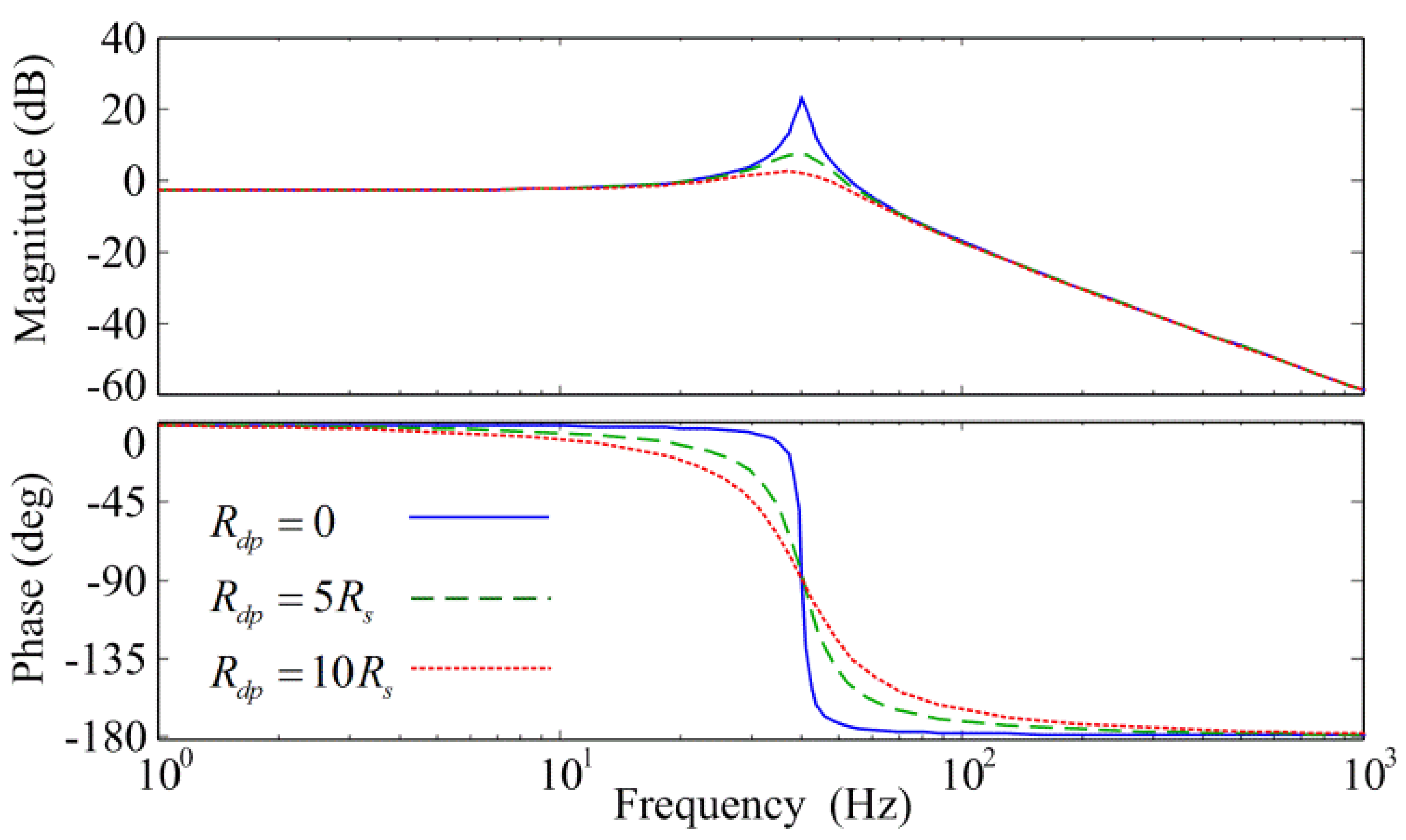
3.2. Current Control Strategy with Active Damping Control
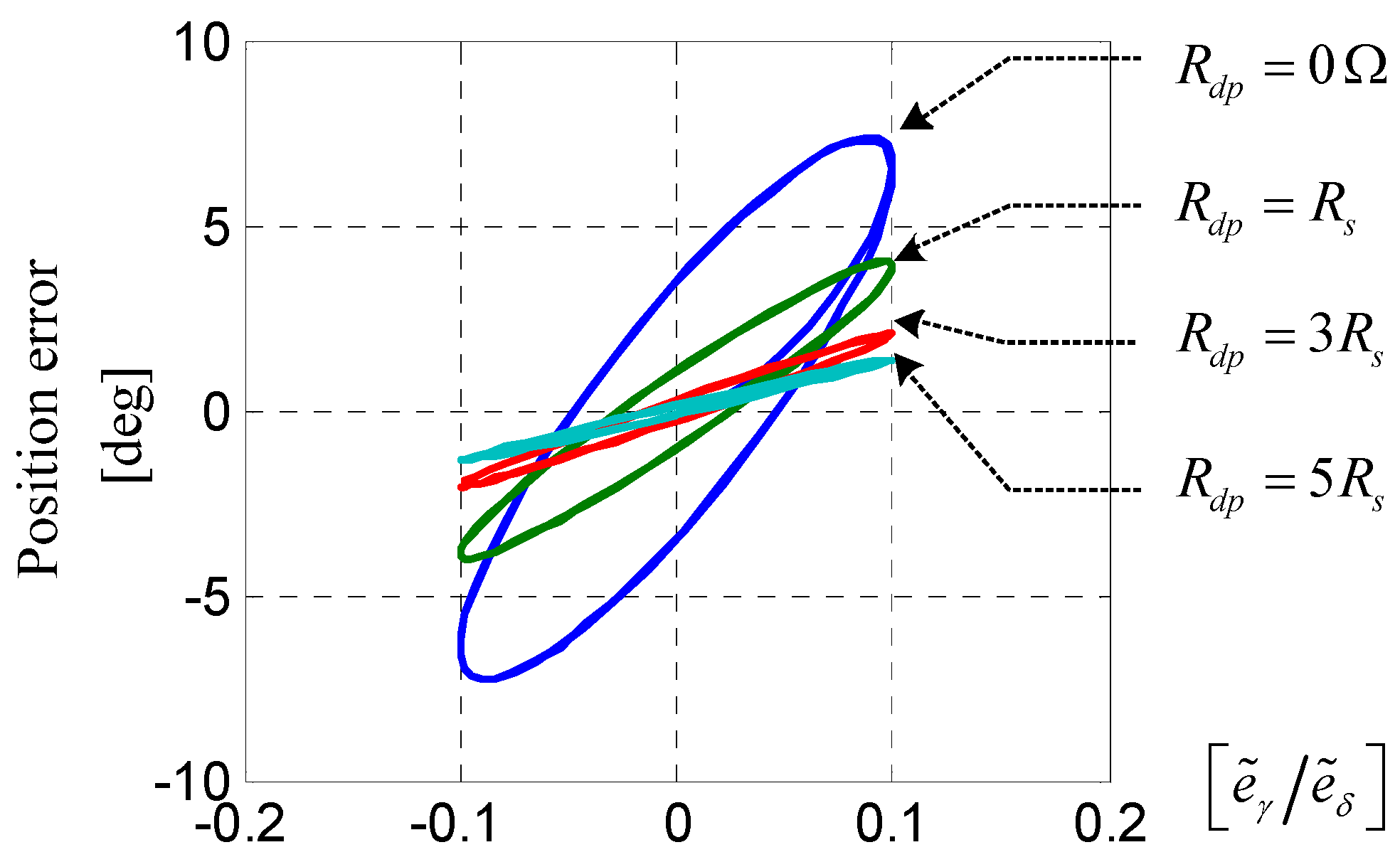
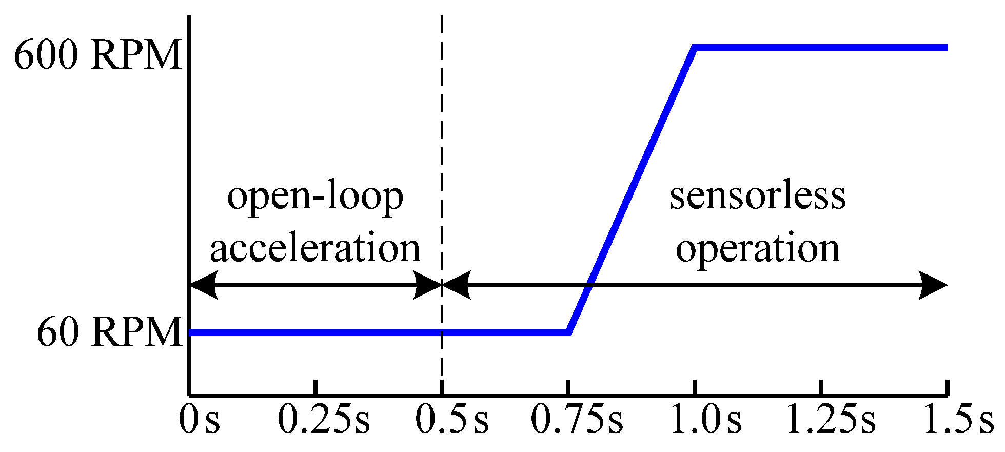
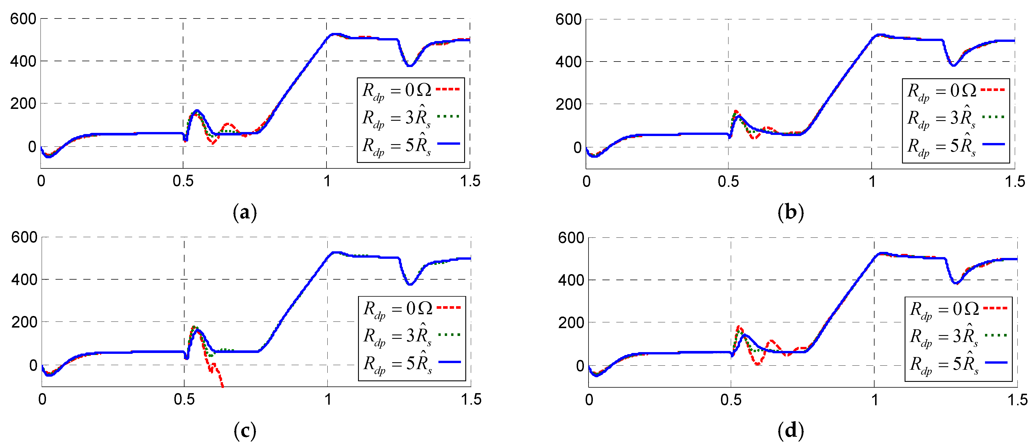
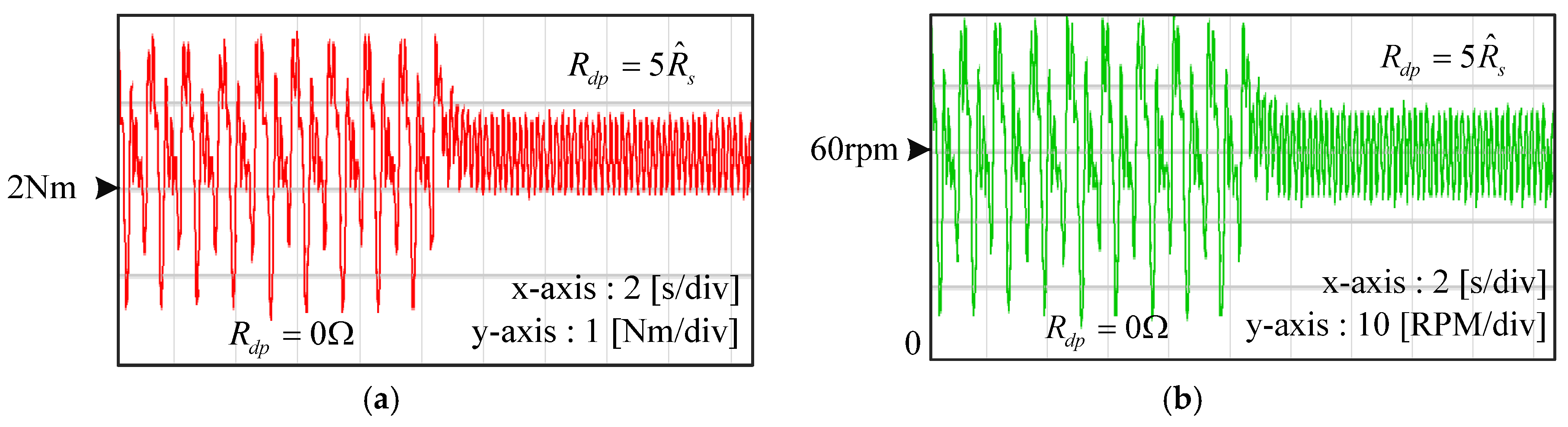
4. Simulation Study
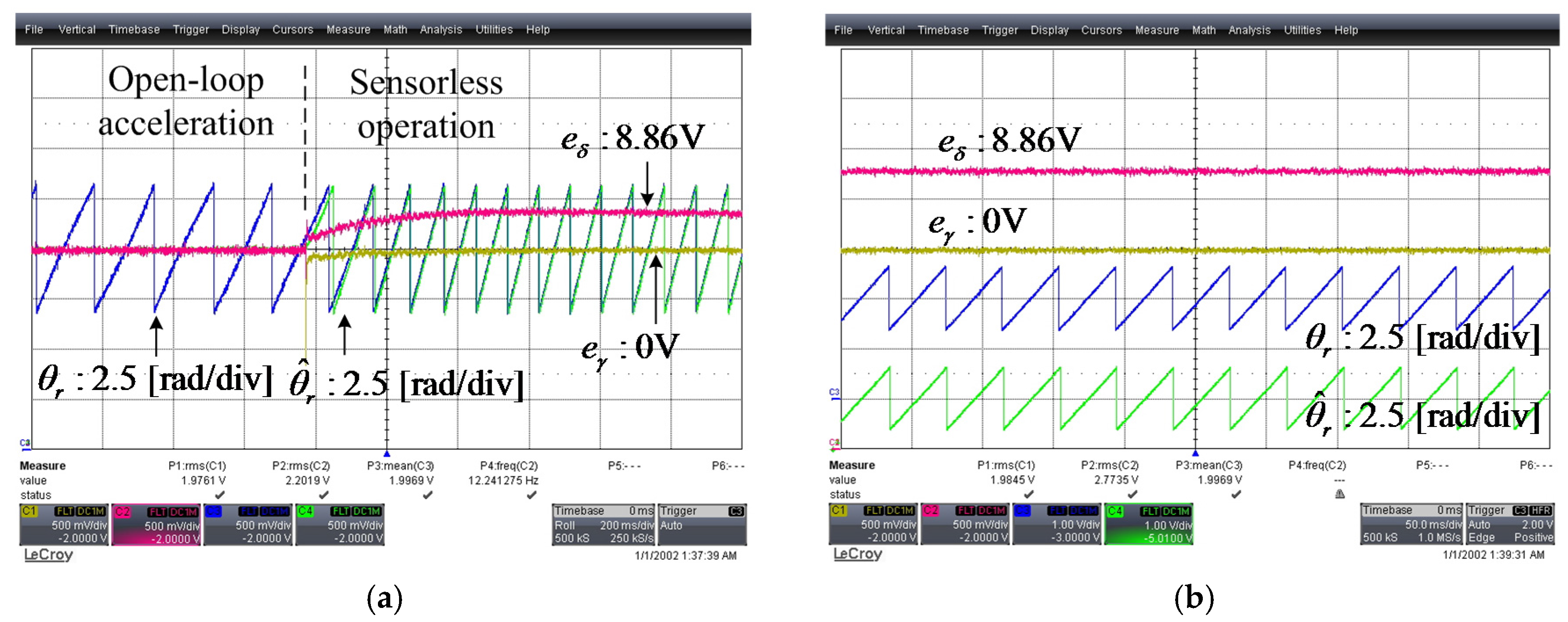
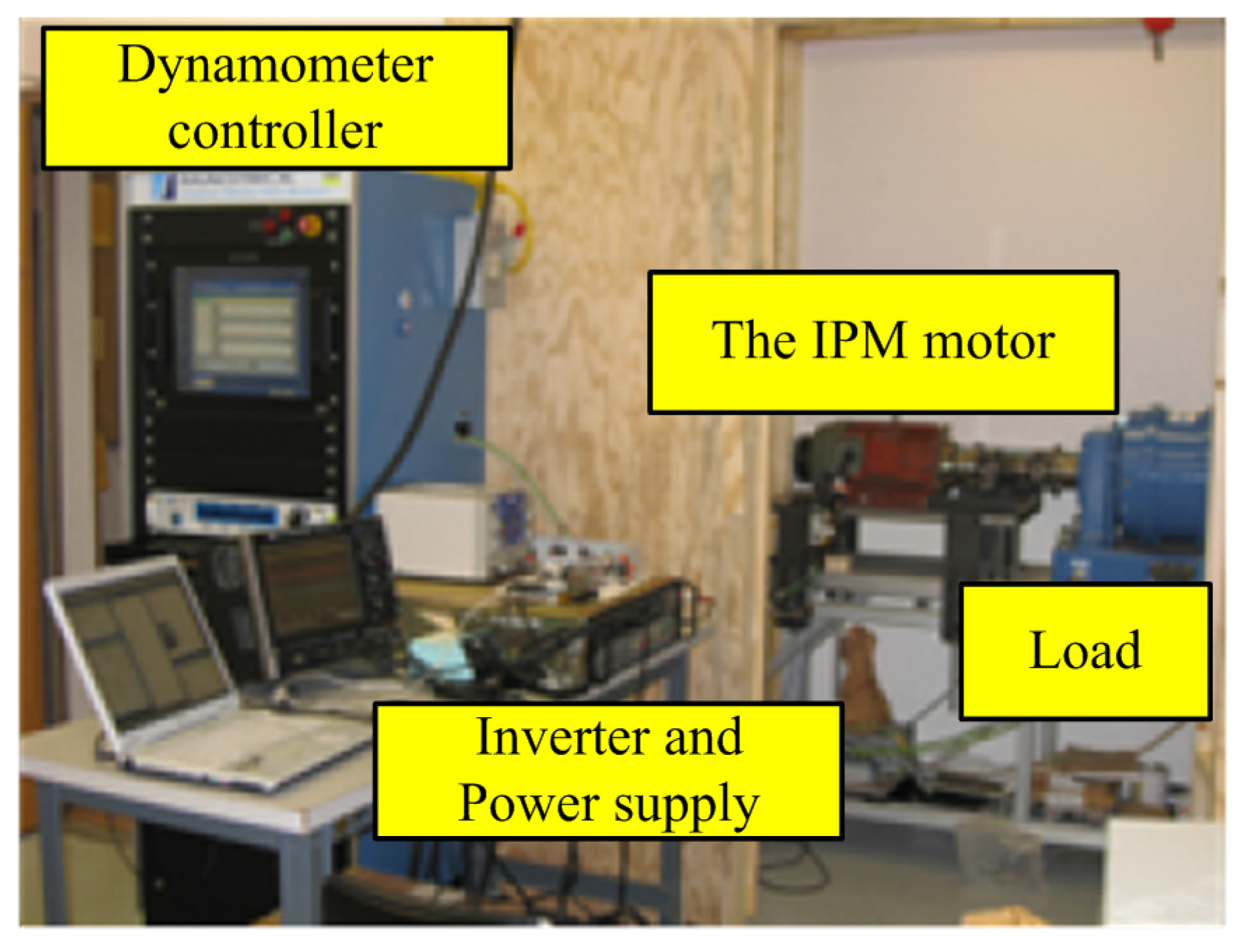
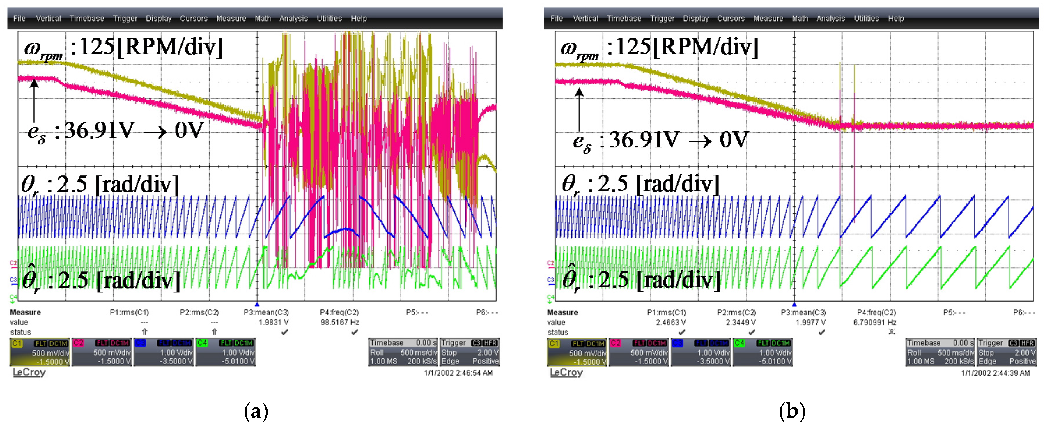
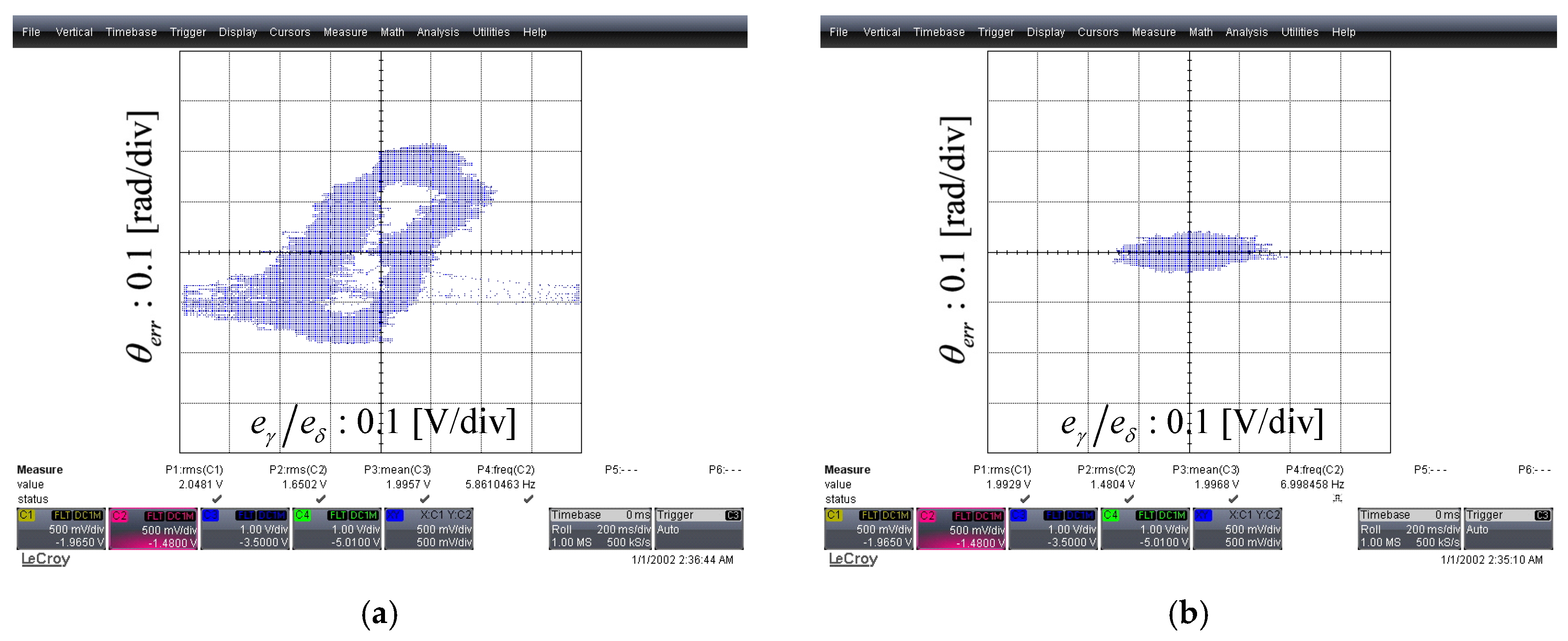
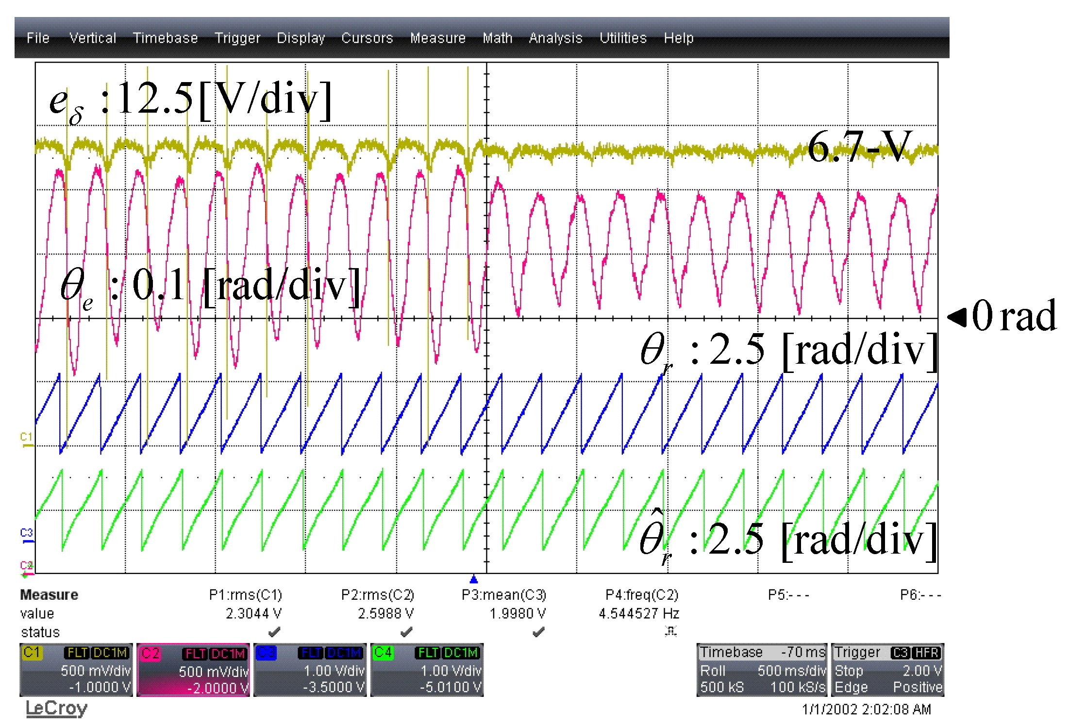
5. Experiments
6. Conclusions
Acknowledgments
Conflicts of Interest
References
- Acarnley, P.P.; Watson, J.F. Review of position-sensorless operation of brushless permanent-magnet machines. IEEE Trans. Ind. Electron. 2006, 53, 352–362. [Google Scholar] [CrossRef]
- Ha, J.I.; Ide, K.; Sawa, T.; Sul, S.K. Sensorless rotor position estimation of an interior permanent-magnet motor from initial states. IEEE Trans. Ind. Appl. 2003, 39, 761–767. [Google Scholar]
- Shi, J.L.; Liu, T.H.; Chang, Y.C. Position control of an interior permanent-magnet synchronous motor without using a shaft position sensor. IEEE Trans. Ind. Electron. 2007, 54, 1989–2000. [Google Scholar]
- Kasa, N.; Watanabe, H. A mechanical sensorless control system for salient-pole brushless DC motor with autocalibration of estimated position angles. IEEE Trans. Ind. Electron. 2000, 47, 389–395. [Google Scholar] [CrossRef]
- Raca, D.; Garcia, P.; Reigosa, D.D.; Briz, F.; Lorenz, R.D. Carrier-signal selection for sensorless control of PM synchronous machines at zero and very low speeds. IEEE Trans. Ind. Appl. 2010, 46, 167–178. [Google Scholar] [CrossRef]
- Reigosa, D.D.; Garcia, P.; Raca, D.; Briz, F.; Lorenz, R.D. Measurement and adaptive decoupling of cross-saturation effects and secondary saliencies in sensorless controlled IPM synchronous machines. IEEE Trans. Ind. Appl. 2008, 44, 1758–1767. [Google Scholar] [CrossRef]
- Yoon, Y.D.; Sul, S.K.; Morimoto, S.; Ide, K. High bandwidth sensorless algorithm for AC machines based on square-wave type voltage injection. In Proceedings of the 2009 IEEE Energy Conversion Congress and Exposition, San Jose, CA, USA, 20–24 September 2009; pp. 2123–2130.
- Hajian, M.; Soltani, J.; Markadeh, G.A.; Hosseinnia, S. Adaptive nonlinear direct torque control of sensorless IM drives with efficiency optimization. IEEE Trans. Ind. Electron. 2010, 57, 975–985. [Google Scholar] [CrossRef]
- Kim, M.; Sul, S.K. An enhanced sensorless control method for PMSM in rapid accelerating operation. In Proceedings of the 2010 International Power Electronics Conference (IPEC), Sapporo, Japan, 21–24 June 2010; pp. 2249–2253.
- Matsui, N. Sensorless PM brushless DC motor drives. IEEE Trans. Ind. Electron. 1996, 43, 300–308. [Google Scholar] [CrossRef]
- Orlowska-Kowalska, T.; Dybkowski, M. Stator-current-based MRAS estimator for a wide range speed-sensorless induction-motor drive. IEEE Trans. Ind. Electron. 2010, 57, 1296–1308. [Google Scholar] [CrossRef]
- Piippo, A.; Hinkkanen, M.; Luomi, J. Analysis of an adaptive observer for sensorless control of interior permanent magnet synchronous motors. IEEE Trans. Ind. Electron. 2008, 55, 570–576. [Google Scholar] [CrossRef]
- Foo, G.; Rahman, M.F. Sensorless sliding-mode MTPA control of an IPM synchronous motor drive using a sliding-mode observer and HF signal injection. IEEE Trans. Ind. Electron. 2010, 57, 1270–1278. [Google Scholar] [CrossRef]
- Mizutani, R.; Takeshita, T.; Matsui, N. Current model-based sensorless drives of salient-pole PMSM at low speed and standstill. IEEE Trans. Ind. Appl. 1998, 34, 841–846. [Google Scholar] [CrossRef]
- Sayeef, S.; Foo, G.; Rahman, M.F. Rotor position and speed estimation of a variable structure direct-torque-controlled IPM synchronous motor drive at very low speeds including standstill. IEEE Trans. Ind. Electron. 2010, 57, 3715–3723. [Google Scholar] [CrossRef]
- Foo, G.; Sayeef, G.; Rahman, M.F. Low-speed and standstill operation of a sensorless direct torque and flux controlled IPM synchronous motor drive. IEEE Trans. Energy Convers. 2010, 25, 25–33. [Google Scholar] [CrossRef]
- Boldea, I.; Paicu, M.C.; Andreescu, G.D.; Blaabjerg, F. Active flux DTFC-SVM sensorless control of IPMSM. IEEE Trans. Energy Convers. 2009, 24, 314–322. [Google Scholar] [CrossRef]
- Raggl, K.; Warberger, B.; Nussbaumer, T.; Burger, S.; Kolar, J.W. Robust angle-sensorless control of a PMSM bearingless pump. IEEE Trans. Ind. Electron. 2009, 56, 2076–2085. [Google Scholar] [CrossRef]
- Rho, M.S.; Kim, S.M. Development of robust starting system using sensorless vector drive for a microturbine. IEEE Trans. Ind. Electron. 2010, 57, 1063–1073. [Google Scholar]
- Yim, J.S.; Lee, W.J.; Sul, S.K.; Yang, H.S.; Kim, J.T. Sensorless vector control of super high speed turbo compressor. In Proceedings of the Twentieth Annual IEEE Applied Power Electronics Conference and Exposition, Austin, TX, USA, 6–10 March 2005; pp. 950–953.
- Zhiqian, C.; Tomita, M.; Doki, S.; Okuma, S. An extended electromotive force model for sensorless control of interior permanent-magnet synchronous motors. IEEE Trans. Ind. Electron. 2003, 50, 288–295. [Google Scholar] [CrossRef]
- Morimoto, S.; Kawamoto, K.; Sanada, M.; Takeda, Y. Sensorless control strategy for salient-pole PMSM based on extended EMF in rotating reference frame. IEEE Trans. Ind. Appl. 2002, 38, 1054–1061. [Google Scholar] [CrossRef]
- Ichikawa, S.; Tomita, M.; Doki, S.; Okuma, S. Sensorless control of synchronous reluctance motors based on extended EMF models considering magnetic saturation with online parameter identification. IEEE Trans. Ind. Appl. 2006, 42, 1264–1274. [Google Scholar] [CrossRef]
- Hasegawa, M.; Yoshioka, S.; Matsui, K. Position sensorless control of interior permanent magnet synchronous motors using unknown input observer for high-speed drives. IEEE Trans. Ind. Appl. 2009, 45, 938–946. [Google Scholar] [CrossRef]
- Ribeiro, L.A.d.S.; Harke, M.C.; Lorenz, R.D. Dynamic properties of back-EMF based sensorless drives. In Proceedings of the 41st IAS Annual Meeting on Industry Applications Conference, Tampa, FL, USA, 8–12 October 2006; pp. 2026–2033.
- Foo, G.; Rahman, M.F. Sensorless direct torque and flux-controlled IPM synchronous motor drive at very low speed without signal injection. IEEE Trans. Ind. Electron. 2010, 57, 395–403. [Google Scholar] [CrossRef]
- Vogelsberger, M.A.; Grubic, S.; Habetler, T.G.; Wolbank, T.M. Using PWM-induced transient excitation and advanced signal processing for zero-speed sensorless control of ac machines. IEEE Trans. Ind. Electron. 2010, 57, 365–374. [Google Scholar] [CrossRef]
- Morimoto, S.; Sanada, M.; Takeda, Y. Mechanical sensorless drives of IPMSM with online parameter identification. IEEE Trans. Ind. Appl. 2006, 42, 1241–1248. [Google Scholar] [CrossRef]
- Mobarakeh, B.N.; Tabar, F.M.; Sargos, F.M. Back EMF estimation-based sensorless control of PMSM: Robustness with respect to measurement errors and inverter irregularities. IEEE Trans. Ind. Appl. 2007, 43, 485–494. [Google Scholar] [CrossRef]
- Inoue, Y.; Yamada, K.; Morimoto, S.; Sanada, M. Effectiveness of voltage error compensation and parameter identification for model-based sensorless control of PMSM. IEEE Trans. Ind. Appl. 2009, 45, 213–221. [Google Scholar] [CrossRef]
- Genduso, F.; Miceli, R.; Rando, C.; Galluzzo, G.R. Back EMF sensorless-control algorithm for high-dynamic performance PMSM. IEEE Trans. Ind. Electron. 2010, 57, 2092–2100. [Google Scholar] [CrossRef]
- Raute, R.; Caruana, C.; Staines, C.S.; Cilia, J.; Sumner, M.; Asher, G.M. Analysis and compensation of inverter nonlinearity effect on a sensorless PMSM drive at very low and zero speed operation. IEEE Trans. Ind. Electron. 2010, 57, 4065–4074. [Google Scholar] [CrossRef]
- Kim, H.; Lorenz, R.D. Synchronous frame PI current regulators in a virtually translated system. In Proceedings of the 39th IAS Annual Meeting on Industry Applications Conference, Seattle, WA, USA, 3–7 October 2004; pp. 856–863.
- Kim, H.; Lorenz, R.D. A virtual translation technique to improve current regulator for salient-pole AC machines. In Proceedings of the 2004 IEEE 35th Annual Power Electronics Specialists Conference, Aachen, Germany, 20–25 June 2004; pp. 487–493.
- Yang, S.M.; Su, P.D. Active damping control of hybrid stepping motor. In Proceedings of the 2001 4th IEEE International Conference on Power Electronics and Drive Systems, Denpasar, Indonesia, 22–25 October 2001; pp. 749–754.
- Yim, J.S.; Sul, S.K.; Bae, B.H.; Patel, N.R.; Hiti, S. Modified current control schemes for high-performance permanent-magnet AC drives with low sampling to operating frequency ratio. IEEE Trans. Ind. Appl. 2009, 45, 763–771. [Google Scholar] [CrossRef]
- Sul, S.K. Control of Electric Machine Drive System, 1st ed.; Brain Korea: Seoul, Korea, 2002. [Google Scholar]


| Parameters | Values |
|---|---|
| Number of poles (P) | 6 |
| Magnet flux linkage () | 0.235 V/(rad/s) |
| d-axis inductance (Ld) | 2.51 mH |
| q-axis inductance (Lq) | 6.94 mH |
| Stator resistance (Rs) | 0.09 |
| Rotor inertia (Jm) | 0.003334 kg·m2 |
| Friction constant (Bm) | 0.425 × 10⁻³·m2/s |
| Rated speed | 1600 rev/min |
| Rated torque | 65 Nm |
| Parameters | Values |
|---|---|
| Switching frequency | 10 kHz |
| Sampling frequency | 10 kHz |
| Current control bandwidth | 300 Hz |
| Position estimator bandwidth | 100 Hz |
| Crossover frequency of the Pseudo integrator and differentiator | 100 Hz |
© 2016 by the author; licensee MDPI, Basel, Switzerland. This article is an open access article distributed under the terms and conditions of the Creative Commons by Attribution (CC-BY) license (http://creativecommons.org/licenses/by/4.0/).
Share and Cite
Cho, Y. Improved Sensorless Control of Interior Permanent Magnet Sensorless Motors Using an Active Damping Control Strategy. Energies 2016, 9, 135. https://doi.org/10.3390/en9030135
Cho Y. Improved Sensorless Control of Interior Permanent Magnet Sensorless Motors Using an Active Damping Control Strategy. Energies. 2016; 9(3):135. https://doi.org/10.3390/en9030135
Chicago/Turabian StyleCho, Younghoon. 2016. "Improved Sensorless Control of Interior Permanent Magnet Sensorless Motors Using an Active Damping Control Strategy" Energies 9, no. 3: 135. https://doi.org/10.3390/en9030135
APA StyleCho, Y. (2016). Improved Sensorless Control of Interior Permanent Magnet Sensorless Motors Using an Active Damping Control Strategy. Energies, 9(3), 135. https://doi.org/10.3390/en9030135