Experimental and Numerical Studies of a High-Head Francis Turbine: A Review of the Francis-99 Test Case

Abstract

Hydraulic turbines are widely used to meet real-time electricity demands. Computational fluid dynamic (CFD) techniques have played an important role in the design and development of such turbines. The simulation of a complete turbine requires substantial computational resources. A specific approach that is applied to investigate the flow field of one turbine may not work for another turbine. A series of Francis-99 workshops have been planned to discuss and explore the CFD techniques applied within the field of hydropower with application to high-head Francis turbines. The first workshop was held in December 2014 at the Norwegian University of Science and Technology, Norway. The steady-state measurements were conducted on a model Francis turbine. Three operating points, part load, best efficiency point, and high load, were investigated. The complete geometry, meshing, and experimental data concerning the hydraulic efficiency, pressure, and velocity were provided to the academic and industrial research groups. Various researchers have conducted extensive numerical studies on the high-head Francis turbine, and the obtained results were presented during the workshop. This paper discusses the presented numerical results and the important outcome of the extensive numerical studies on the Francis turbine. The use of a wall function assuming equilibrium between the production and dissipation of turbulence is widely used in the simulation of hydraulic turbines. The boundary layer of hydraulic turbines is not fully developed because of the continuously-changing geometry and large pressure gradients. There is a need to develop wall functions that enable the estimation of viscous losses under boundary development for accurate simulations. Improved simulations and results enable reliable estimation of the blade loading. Numerical investigations on leakage flow through the labyrinth seals were conducted. The volumetric efficiency and losses in the seals were determined. The seal leakage losses formulated through analytical techniques are sufficient.

1. Introduction

Computational fluid dynamic (CFD) techniques have been used to study the flow conditions inside hydraulic turbines over the past three decades [1]. The numerical modeling of hydraulic turbines is a challenging task because a specific modeling approach applied to investigate a certain operating condition does not necessarily work for another operating condition. Small changes in discharges and/or head significantly affect the flow conditions inside the turbine. There are several challenges for hydraulic turbine modeling in terms of obtaining useful results.

An open test case allowing researchers to interact to address such questions is, thus, necessary to develop the numerical capacity for the study of hydraulic turbines. The main objective of the Francis-99 test case is to provide an open platform to industrial and academic researchers to explore and develop the capabilities of CFD techniques within the field of hydropower research. The Francis-99 test case consists of a high-head Francis turbine model, whose geometry, together with meshing and measurement (pressure and velocity) data, are available for academic research purpose [2].

The first workshop attempted to determine the state of the art in the simulation of high-head Francis turbines under steady operations, namely, at part load (PL), best efficiency point (BEP), and high load (HL). The motivation resided in the continuous development of more powerful computers, thereby facilitating the use of more advance turbulence models and accurate numerical schemes. Efficiency, pressure, and velocity measurements were conducted on the Francis-99 test case at the Water Power Laboratory, Norwegian University of Science and Technology (NTNU), Norway. Prepared three-dimensional geometry and hexahedral meshes of the complete turbine were provided to facilitate the numerical simulations. Approximately 50 people participated in the workshop, and 14 papers were presented using various codes, turbulence models, and turbine modeling approaches. This paper provides an important summary of the numerical results presented in the first workshop.

2. Test Case

2.1. Test Rig

The measurements were conducted on a test rig available at the Water Power laboratory, NTNU. The hydraulic system is capable of generating a head of up to 14 m for the open loop and 100 m for the closed loop. During open-loop turbine operation, water is pumped at a constant discharge to the overhead tank and allowed to flow down to the turbine. The water level is maintained as constant in the tank through an overflow piping system. For the closed-loop system, feed pumps generate the required head, and water recirculates in the closed piping. The open-loop and closed-loop systems were used for the pressure and velocity measurements, respectively. The head across the turbine was similar for both measurements. Under the BEP operating condition, the head and discharge were 12 m and 0.2 m³·s⁻¹, respectively.

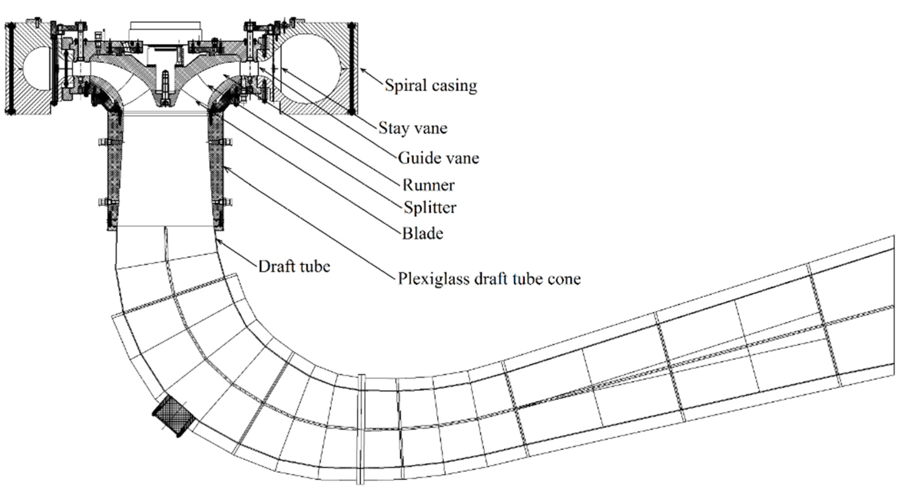
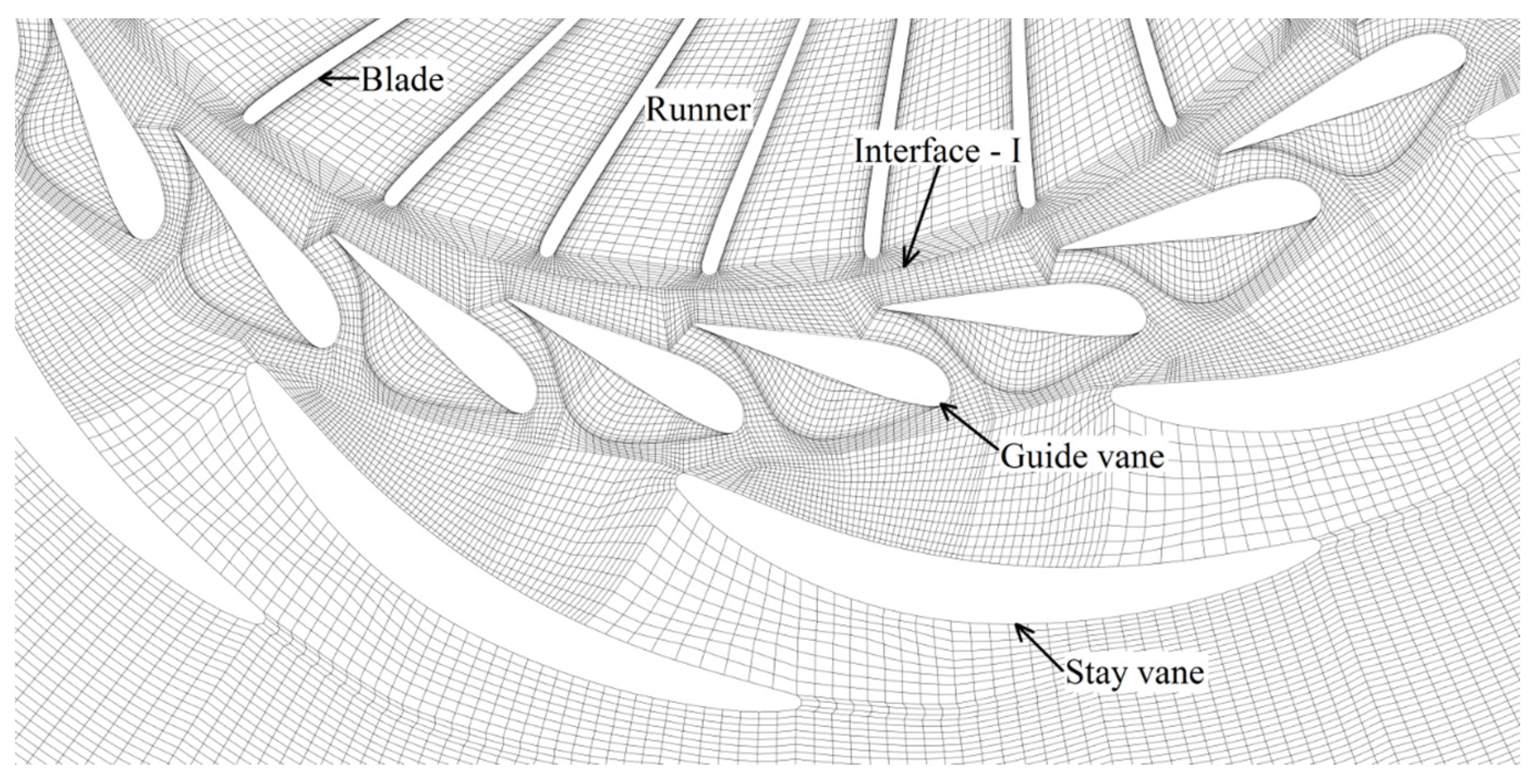
Figure 1 shows a two-dimensional view of the investigated Francis turbine. The turbine includes a spiral casing, a distributor with 14 stay vanes integrated into the spiral casing and 28 guide vanes, a runner with 15 blades and 15 splitters, and an elbow-type draft tube. The turbine is a reduced-scale (1:5.1) model of the prototype Francis turbines operating at the Tokke power plant, Norway. A total of four prototypes are in operation at the power plant, and each generates 110 MW at BEP. Table 1 shows the operating parameters of the model and prototype turbines. The dimensionless specific speed (N_QE) of the prototype turbine is 0.073.

$$N_{QE}=\frac{n\cdot Q^{0.5}}{E^{0.75}}(-)$$

(1)

where n is the runner speed in revolutions per second, Q is the discharge in m³·s⁻¹, g is the gravity constant in m·s⁻², and E is the specific hydraulic energy in J·kg⁻¹; E = gH, g = 9.82 m·s⁻².

Table 1. Operating parameters of the model and prototype Francis turbines at BEP.

Operating Parameter	Symbol	Model	Prototype	Unit
Head	H	12	377	m
Discharge	Q	0.2	31	m3·s−1
Power	P	0.022	110 × 4	MW
Runner diameter	d	0.349	1.778	M
Runner speed	n	335	375	rpm
Reynolds number	Re	1.8 × 106	4.1 × 107	-

Table 1. Operating parameters of the model and prototype Francis turbines at BEP.

Operating Parameter	Symbol	Model	Prototype	Unit
Head	H	12	377	m
Discharge	Q	0.2	31	m3·s−1
Power	P	0.022	110 × 4	MW
Runner diameter	d	0.349	1.778	M
Runner speed	n	335	375	rpm
Reynolds number	Re	1.8 × 106	4.1 × 107	-

Figure 1. Two-dimensional view of the investigated model Francis turbine.

Figure 1. Two-dimensional view of the investigated model Francis turbine.

2.2. Instrumentation

The model Francis turbine was equipped with instruments and sensors required to perform the model test according to IEC 60193 [3]. Two pressure transducers were used to acquire the turbine inlet pressure and differential pressure across the turbine. A torque transducer was used to measure the generator input torque, and another transducer was used to measure the frictional torque in the thrust block and radial bearings. The runner speed was acquired using a disk with slots, which provided pulses corresponding to the instantaneous angular speed. All of the data required to plot the turbine hill chart were acquired at a sampling rate of 1.45 Hz.

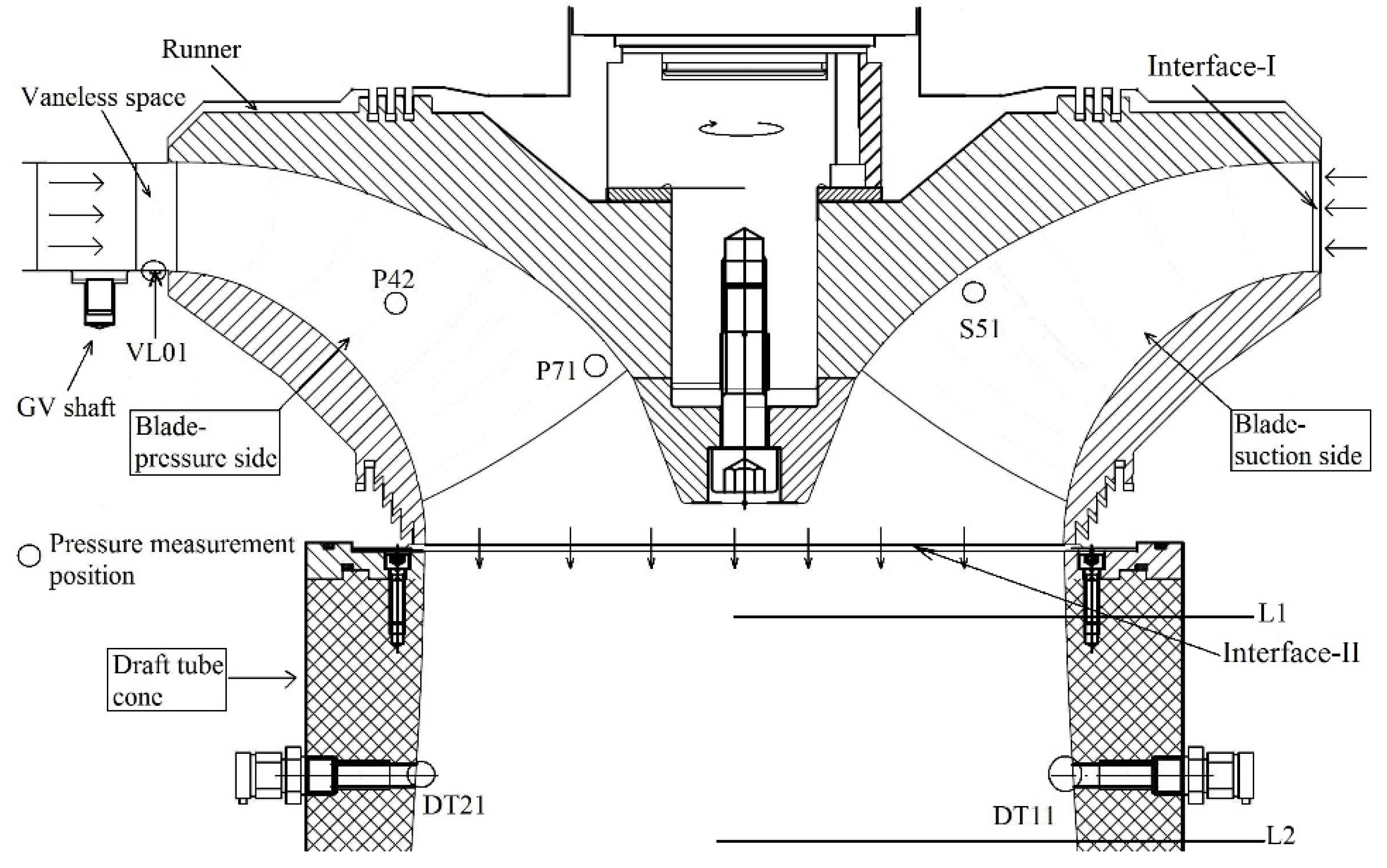
Additionally, six pressure sensors were mounted at different locations inside the turbine. Figure 2 shows the locations of the pressure sensors. A miniature pressure sensor, VL01, was flush mounted in the vaneless space to acquire pressure pulsations generated by the rotor-stator interactions. Two miniature pressure sensors, P42 and P71, were mounted on the blade pressure side and the trailing edge, respectively. The other miniature pressure sensor, S51, was mounted on the blade suction side. Pressure values from the P42, P71, and S51 sensors were acquired using a SRI-500e wireless telemetry system from Summation Research. The remaining two pressure sensors, DT11 and DT21, were mounted on the wall of the draft tube cone. Both sensors were located on a plane at a distance of 0.126 m from the runner outlet and with an angular separation of 180° from each other. Data from all of the pressure sensors were acquired at a rate of 2083 Hz.

Two-dimensional laser Doppler velocimetry (LDV) and particle image velocimetry (PIV) were used for the velocity measurements in the draft tube cone [4]. The utilized LDV system is composed of a Spectra-Physics Model 177G laser and is equipped with a burst spectrum analyzer from Dantec Dynamics. The perpendicularity of the LDV probe was checked using optical methods with an accuracy of 0.2°. The front lens had a focal length of 310 mm. Seeding particles, Expancel 46 WU 20, with an average diameter of 6 µm were used. The measurement sections L1 and L2 are shown in Figure 2 and were are at a distance of 0.064 and 0.382 m from the runner outlet, respectively. For the 2D PIV system, pulse light sheets with a thickness of approximately 3 mm were generated by a Litron Laser NANO L100-50PIV. The illuminated field was recorded by a 4-MP camera (VC-4MC-M180). TSI seeding particles, with a density of 1.016 g/cc, refractive index of 1.52 and mean diameter of 55 µm, were used for the measurements. The PIV measurement data were sampled at the rate of 40 Hz. A total of 750 paired images with a time difference of 200 µs were recorded at each measurement section.

Figure 2. Locations of the mounted pressure sensors in the model Francis turbine during measurements at the BEP, HL, and PL; VL01-vaneless space, P42-blade pressure side, P71-blade trailing edge, S51-blade suction side, DT11 and DT21-draft tube; L1 and L2 correspond to the measurement sections for LDV. The distance of L1 and L2 are 0.064 and 0.382 m from the runner outlet, respectively.

Figure 2. Locations of the mounted pressure sensors in the model Francis turbine during measurements at the BEP, HL, and PL; VL01-vaneless space, P42-blade pressure side, P71-blade trailing edge, S51-blade suction side, DT11 and DT21-draft tube; L1 and L2 correspond to the measurement sections for LDV. The distance of L1 and L2 are 0.064 and 0.382 m from the runner outlet, respectively.

2.3. Calibration and Uncertainty Analysis

Calibration and uncertainty analysis for the sensors used for the measurements were performed before the measurements were conducted. IEC 60193 [3] was followed for the calibration, uncertainty analysis, and measurements on the model Francis turbine. The calibration of the instruments and sensors was performed for the magnetic flow meter, torque measurement sensors, runner speed measurement sensor, inlet and differential pressure transducers, and miniature pressure sensors. The total uncertainty was obtained by combining the systematic and random uncertainties, as shown in Equation (2), and was calculated to be ±0.15% [5,6,7]:

$${\left({\delta }_{{\eta }_h}\right)}_t=\pm \sqrt{{\left({\delta }_{{\eta }_h}\right)}_s^2+{\left({\delta }_{{\eta }_h}\right)}_r^2}$$

(2)

The maximum systematic uncertainties of the sensors P42, P71, and S51 mounted in the runner were 0.62%, 0.45%, and 0.22% of the measured value, respectively. The maximum systematic uncertainty of sensors VL01, DT11, and DT21 located in the stationary domains was 0.15% of the measured value.

In order to evaluate the repeatability of the velocity measurements, axial and radial velocity profiles were prepared using two different windows. The measurements were performed three times at each window. The measurements for each window were performed on different days while the test rig was operating continuously. The highest level of discrepancies in both components is found close to the central part of the draft tube where the velocity is higher than close to the wall region. The perpendicularity of the sections was checked with optical methods with an accuracy of 0.2°. Each velocity profile was investigated with 16 measurement points along the radius for BEP and HL, and at 26 points for PL. The large number of measurement points at PL was necessary to capture the high velocity gradients. The recording time was reduced to 600 s for the last measurements. The velocity data in terms of profiles at the L1 and L2 sections were provided with 95% confidence level. Detailed information regarding calibration procedure and uncertainty analysis can be found in the literature [4].

2.4. Measurements

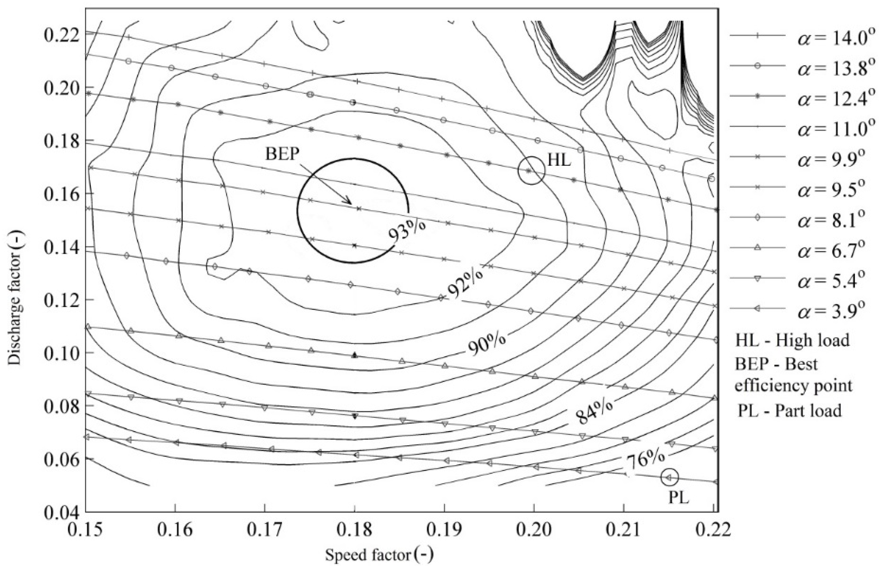
Steady-state measurements on the model Francis turbine were conducted. Figure 3 shows the constant efficiency hill chart of the model Francis turbine. The hill chart covers 150 operating points, including 10 angular positions of the guide vanes ranging from 3.9° to a maximum of 14° and 15 values of the runner angular speed for each angular position of the guide vanes. The maximum hydraulic efficiency was 93% at the BEP, n_ED = 0.18, and Q_ED = 0.15. Three operating points were investigated for the Francis-99 workshop: part load (PL), BEP, and high load (HL). The guide vane angular positions for the PL, BEP and HL correspond to 3.9°, 9.9°, and 12.4°, respectively. The discharge values were 0.071, 0.2, and 0.22 m³·s⁻¹ for the PL, BEP and HL, respectively.

Figure 3. Constant efficiency hill diagram of the model Francis turbine (D = 0.349 m, H =12 m); n_ED = 0.18 is the dimensionless synchronous speed of the model turbine runner, BEP refers to the best efficiency point (n_ED = 0.18, and Q_ED = 0.15), and α corresponds to the angular position of the guide vanes in degrees [5].

Figure 3. Constant efficiency hill diagram of the model Francis turbine (D = 0.349 m, H =12 m); n_ED = 0.18 is the dimensionless synchronous speed of the model turbine runner, BEP refers to the best efficiency point (n_ED = 0.18, and Q_ED = 0.15), and α corresponds to the angular position of the guide vanes in degrees [5].

Equation (3) was used for the computation of the hydraulic efficiency. The values of the torque (T), runner angular speed (ω), and discharge to the turbine (Q) were acquired during the measurements. The value of the pressure (∆p) was acquired by the differential pressure transducer. The head (H) was estimated using Equation (5). To construct the hill diagram, the dimensionless values of the speed (n_ED) and discharge (Q_ED) factors were estimated using Equations (6) and (7), respectively:

$${\eta }_M=\frac{T\cdot \omega }{p_M\cdot Q}(-)$$

(3)

$$p_M=\Delta p+\frac{\rho \cdot Q^2}{2}\cdot \left(\frac{1}{A_1^2}-\frac{1}{A_2^2}\right)(\mathrm{Pa})$$

(4)

$$H=\frac{p_M}{\rho \cdot g}(\text{m})$$

(5)

$$n_{ED}=\frac{\omega \cdot D}{\sqrt{E}}(-)$$

(6)

$$Q_{ED}=\frac{Q}{D^2\cdot \sqrt{E}}(-)$$

(7)

$$E=g\cdot H(\text{J}·{\text{kg}}^{-1})$$

(8)

where g is gravity in m²·s⁻¹, ρ is the density of water in kg·m⁻³, D is the model runner reference diameter in m, and A is the cross sectional area at the measurement sections in m².

3. Numerical Modeling

3.1. Geometry

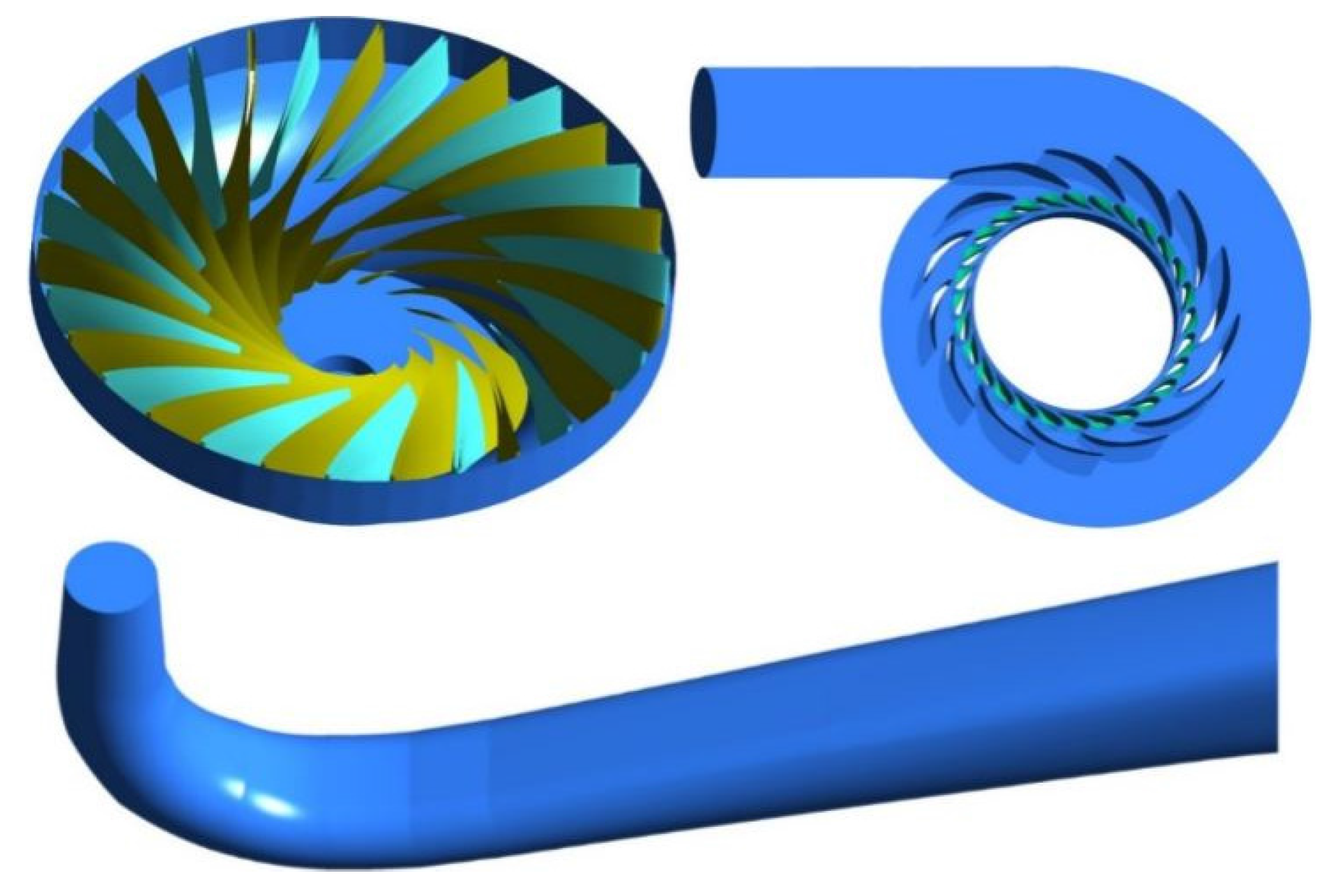
The three-dimensional geometry was prepared using an available AutoCAD drawing of the complete turbine. The geometry includes the spiral casing, distributor, runner, and draft tube. Figure 4 shows the three-dimensional model of the Francis turbine. The geometry was prepared using the ANSYS ICEM CFD CAD software. Some assumptions were made in the numerical model to reduce the complexities; e.g., the fillet radius on the stay vanes, splitters, and blades were not modeled. Further, labyrinth seals were not included because modeling the fluid flow in the labyrinth seals requires substantial computational power. The prepared geometry of the turbine for the three operating points was provided to the researchers. A two-dimensional AutoCAD drawing of the turbine was also provided for researchers interested in preparing a geometry using their own software and techniques.

Figure 4. Three-dimensional model of the Francis turbine; (top left): runner with blades and splitters; (top right): spiral casing with distributor, (bottom): draft tube.

Figure 4. Three-dimensional model of the Francis turbine; (top left): runner with blades and splitters; (top right): spiral casing with distributor, (bottom): draft tube.

Several researchers at the workshop applied different numerical modeling approaches. The approaches were mainly dependent on the operating point of the turbine. For example, the distributor and runner were modeled for the flow analysis in the vaneless space, whereas a blade passage and/or draft tube were modeled to study the vortex rope at part load operation. Two research groups had modeled the complete turbine with labyrinth seals. Through extensive use of numerical modeling techniques and turbulence modelling, some of them were tested and applied for the workshop.

3.2. Mesh Creation and Quality

The hexahedral mesh in the complete turbine was prepared using ICEM CFD. A three-dimensional blocking technique was applied to create the mesh. The turbine was divided into three domains: the spiral casing with distributor, runner, and draft tube. The mesh was independently created in all domains. Figure 5 shows the hexahedral mesh in the section containing the distributor and runner. The total number of nodes was approximately 12 million for the complete turbine, including 5 million nodes in the runner. A fine mesh close to the boundaries and in the complex passages of the turbine was created. The pre-mesh blocks were provided to the researchers and allowed the creation of a finer mesh and use of different node spacing in the expansion layer from a no-slip-type wall or other boundary locations. Table 2 shows overall mesh information and quality of the pre-mesh provided to the workshop participants. The provided pre-mesh in the turbine was coarse for some research groups. However, the research groups have improved the mesh quality and density as per the availability of computational resources and requirement of mesh expansion for proper resolution of turbulence scales. 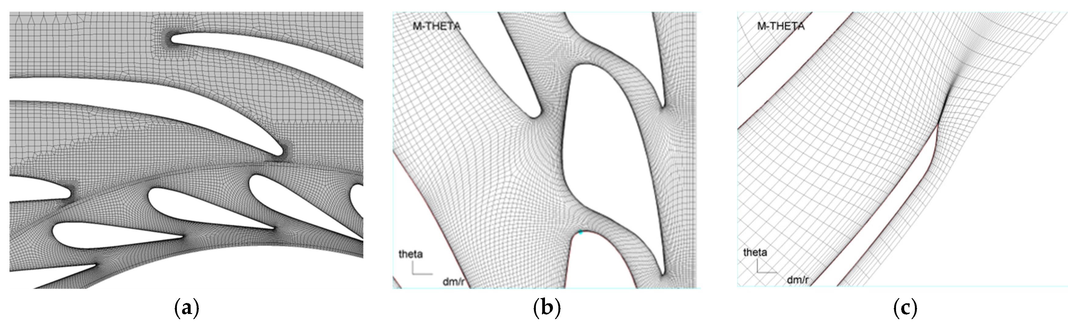Figure 6 shows an example of improved mesh in the distributor and guide vane passages of the turbine.

Table 2. Statistics and quality of the mesh provided for the numerical simulations.

Mesh Statistics and Quality Parameters	Distributor	Runner	Draft Tube
Element Type	Hexahedral	Hexahedral	Hexahedral
Elements (million)	3.78	4.9	3.7
Nodes (million)	3.61	4.64	3.64
First node (mm)	0.65	0.19	0.32
Element incremental ratio	1.5	1.3	1.5
y+ (at the BEP operation)	65	11	40
Aspect ratio (0–100)	1–40	1–41.3	1–37.5
Mesh expansion factor (0–20)	0.1–8.59	0.1–4.57	0.99–3.73
Minimum orthogonality (0–90)	37.7	43.5	70.4

Table 2. Statistics and quality of the mesh provided for the numerical simulations.

Mesh Statistics and Quality Parameters	Distributor	Runner	Draft Tube
Element Type	Hexahedral	Hexahedral	Hexahedral
Elements (million)	3.78	4.9	3.7
Nodes (million)	3.61	4.64	3.64
First node (mm)	0.65	0.19	0.32
Element incremental ratio	1.5	1.3	1.5
y+ (at the BEP operation)	65	11	40
Aspect ratio (0–100)	1–40	1–41.3	1–37.5
Mesh expansion factor (0–20)	0.1–8.59	0.1–4.57	0.99–3.73
Minimum orthogonality (0–90)	37.7	43.5	70.4

Figure 5. Hexahedral mesh in the distributor and runner of the model Francis turbine. Mesh cut is at the distributor floor.

Figure 5. Hexahedral mesh in the distributor and runner of the model Francis turbine. Mesh cut is at the distributor floor.

Figure 6. Improved mesh in the distributor and guide vane passages [6]. (a) mesh (hex dominant) in stay vane and guide vane passages at the mid-plane of spiral casing; (b) mesh (hexahedral) in guide vane passages; and (c) mesh (hexahedral) in the blade passage.

Figure 6. Improved mesh in the distributor and guide vane passages [6]. (a) mesh (hex dominant) in stay vane and guide vane passages at the mid-plane of spiral casing; (b) mesh (hexahedral) in guide vane passages; and (c) mesh (hexahedral) in the blade passage.

Similar to geometry creation, certain research groups used their own software and techniques to create the mesh. Meshes with different densities, generating between 3 million and 48 million nodes, were created. Table 3 shows the modeling approaches, mesh densities, and dimensionless node distances from the boundary (y⁺) presented at the workshop. Three modeling approaches have been applied: (1) complete turbine modeling; (2) component modeling; and (3) passage modeling. In the complete turbine modeling, the spiral casing, stay vanes, guide vanes, runner with blades and splitters, and draft tube of the turbine were modeled. In the component modeling approach, the runner and draft tube were modeled. In the passage modeling approach, a passage of the distributor and the runner blade were modeled. A majority of the simulations were performed using the complete turbine modeling approach. The maximum mesh density for the complete turbine generated approximately 48 million nodes [8]. Total nine research groups [6,9,10,11,12,13,14,15,16] have performed their own mesh scaling test as stated in Table 3, “Mesh scaling test”. The simulations were performed after the mesh scaling test. The dimensionless node spacing from the wall was dependent on the type of turbulence model analyzed in the numerical study. For the simulations performed using the SST and/or SAS models, the y⁺ value was maintained as less than one [6]. For the RANS models with the scalable wall function, the average y⁺ value was approximately 300. The minimum angle, maximum aspect ratio, and maximum volume change are in the corresponding turbine domain are presented. Codes/solvers have different structure (e.g., cell-centered, vertex-centered), Therefore, the same mesh has a different quality function of the solver considered. Each solver recommends certain criteria for the simulations and researchers are generally trying to follow those guidelines [17,18]. Ansys CFX solver recommends an aspect ratio generally less than 10,000, minimum angle of element greater than 18 degrees, and volume expansion lower than 10 [19]. Detailed information about the mesh quality is well documented in the literature [7,19].

Table 3. Summary of the applied modeling approaches, meshing, and dimensionless node distance from the boundary (y⁺) and the mesh quality.

Reference	Modeling Approaches	Mesh (Million)	Mesh Scaling Test	y+	Angle (°)	Aspect Ratio	Volume Change
[6]	Complete turbine Guide vane and blade passage	9.6 3.6	Yes	~200 <1	29.1	1383	5
[20]	Complete turbine	12.5	No	~300	41	350	9
[21]	Complete turbine Blade passage	13 0.5	No	~300 ~300	41	350	9
[9]	Runner and draft tube	6	Yes	~300	--	--	--
[10]	Completer turbine	20.2	Yes	~53	15.2	254	101
[11]	Complete turbine	14.6	Yes	~6	--	--	--
[8]	Complete turbine and labyrinth seals	48.4	No	--	--	--	--
[12]	Complete turbine	4.2	Yes	>100	11	--	--
[13]	Spiral casing, distributor, blade passage, and draft tube	11	Yes	~22	28	1421	97
[14]	Complete turbine	16.5	Yes	~22	28	1422	97
[15]	Guide vane and blade passage, and draft tube	12.35	Yes	--	41	350	9
[22]	Complete turbine	13	No	--	41	350	97
[16]	Guide vane and blade passage	13.4	Yes	<88	33.7	66.7	1.77

Table 3. Summary of the applied modeling approaches, meshing, and dimensionless node distance from the boundary (y⁺) and the mesh quality.

Reference	Modeling Approaches	Mesh (Million)	Mesh Scaling Test	y+	Angle (°)	Aspect Ratio	Volume Change
[6]	Complete turbine Guide vane and blade passage	9.6 3.6	Yes	~200 <1	29.1	1383	5
[20]	Complete turbine	12.5	No	~300	41	350	9
[21]	Complete turbine Blade passage	13 0.5	No	~300 ~300	41	350	9
[9]	Runner and draft tube	6	Yes	~300	--	--	--
[10]	Completer turbine	20.2	Yes	~53	15.2	254	101
[11]	Complete turbine	14.6	Yes	~6	--	--	--
[8]	Complete turbine and labyrinth seals	48.4	No	--	--	--	--
[12]	Complete turbine	4.2	Yes	>100	11	--	--
[13]	Spiral casing, distributor, blade passage, and draft tube	11	Yes	~22	28	1421	97
[14]	Complete turbine	16.5	Yes	~22	28	1422	97
[15]	Guide vane and blade passage, and draft tube	12.35	Yes	--	41	350	9
[22]	Complete turbine	13	No	--	41	350	97
[16]	Guide vane and blade passage	13.4	Yes	<88	33.7	66.7	1.77

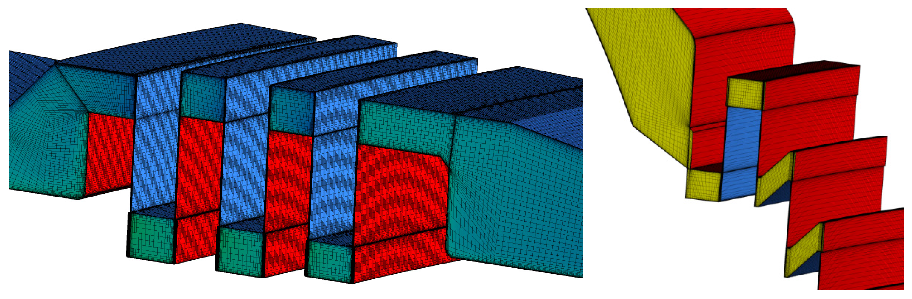
A hexahedral mesh was created in the labyrinth seals by two research groups to investigate the flow leakage losses in the turbine [8,11,13]. Figure 7 shows the mesh of the upper and lower labyrinth seals of the turbine runner. Close to the wall of the labyrinth seals, a fine mesh was created to improve the velocity profile from the no-slip boundaries. Both seals include 63 million nodes, and the results presented in the workshop are discussed in Section 6.,3 Flow analysis in labyrinth seals.

Figure 7. Hexahedral mesh of the upper and lower labyrinth seals of the model Francis turbine runner [8].

Figure 7. Hexahedral mesh of the upper and lower labyrinth seals of the model Francis turbine runner [8].

3.3. Mesh Scaling Test

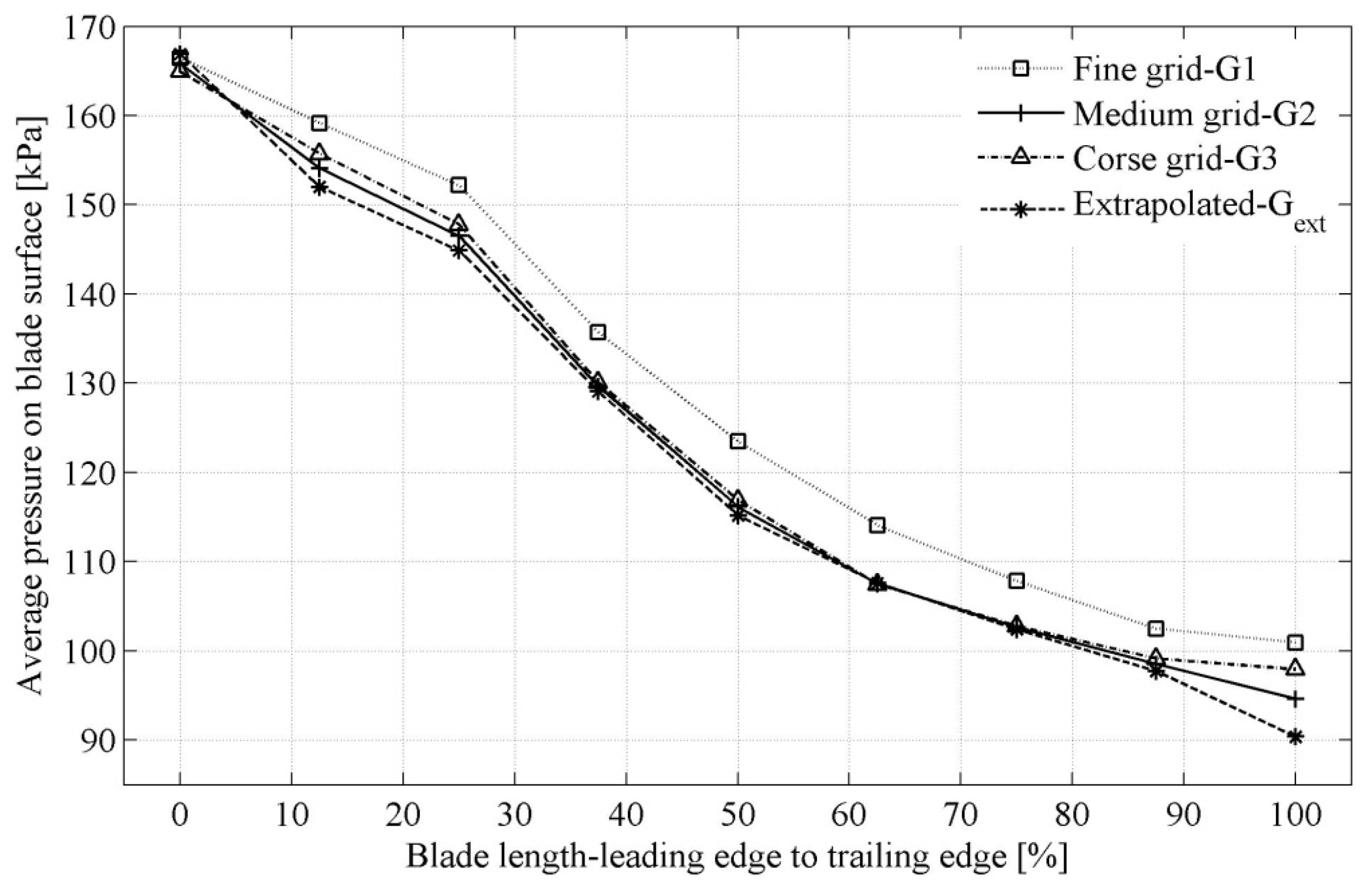
Numerical study on the Francis turbine was performed before distributing the turbine geometry and mesh [7]. Hexahedral meshes of three different densities, 20, 10, and 5 million nodes, were created in the complete turbine. The simulations were performed at the BEP. Mesh types G1, G2, and G3 correspond to 20, 10, and 5 million nodes, respectively. Detailed analysis of the mesh with grid convergence index method was carried out [23]. Figure 8 shows the pressure distribution along the blade length for three densities of the mesh. For the fine grid, the maximum discretization uncertainty was 5.81% at the blade trailing edge, whereas the medium grid (10 million nodes) showed the maximum uncertainty of 4.1%. The medium grid (G₂) showed results of hydraulic efficiency close to the experimental value. The medium grid with improved quality was distributed to the Francis-99 research groups.

Figure 8. Pressure distribution on the blade for three grid densities and extrapolated pressure [5].

Figure 8. Pressure distribution on the blade for three grid densities and extrapolated pressure [5].

As summarized in Table 3, some of the research groups performed their own mesh scaling tests before the final simulations. Nicolle and Cupillard [6] created their own geometry and mesh of the Francis turbine. Passages of the distributor and the runner were modeled. Mesh independency tests were conducted at BEP using 1.1 million, 2.2 million, 4.6 million, and 9.6 million nodes. The hydraulic efficiency and the runner output power were used to verify the results. A very small difference, less than 0.01%, in the hydraulic efficiency was obtained when using 4.6 million and 9.6 million nodes. A mesh with 9.6 million nodes was selected for the simulations under PL and HL conditions. The simulations were performed using both standard k-ε and shear-stress transport (SST) models. The standard k-ε model showed large differences and randomness in the power output. Further, the influence of the y⁺ value and mesh resolution near the boundaries was investigated. The y⁺ value and the mesh resolution were found to possibly affect the flow field. 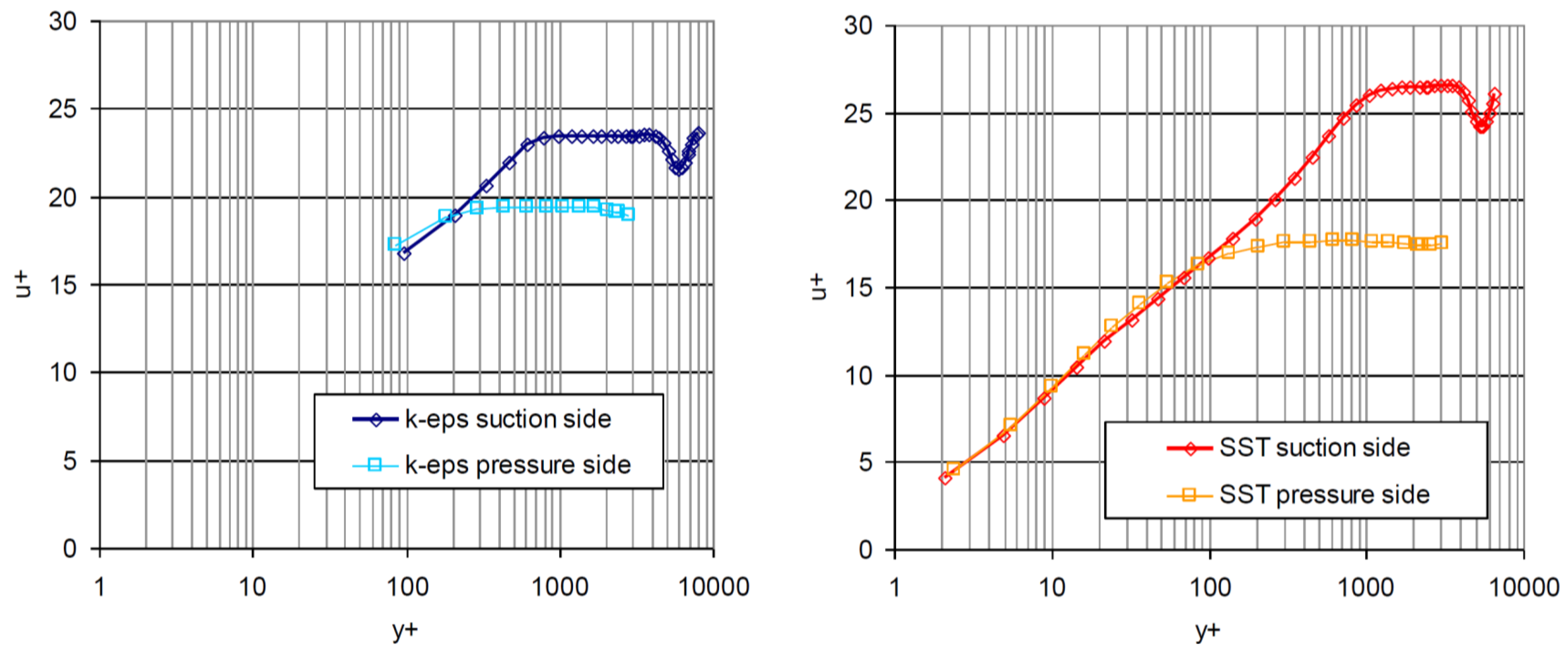Using the SST model, the computed power is dependent on the y⁺ value of the first cell thickness. Figure 9 shows the near-boundary velocity variation on the pressure and suction sides of a guide vane for the different values of y⁺. According to author, the boundary layer on the pressure and suction sides of the guide vane was approximately 0.2 and 0.6 mm, respectively [6]. The location of the profile was 90% of chord length from the leading of the guide vane at mid-plane, which is 10.3 mm before the trailing edge.

Figure 9. Boundary layer estimation on the pressure and suction sides of the guide vane with different y⁺ values and turbulence models [6]. u⁺ is the dimensionless velocity: the velocity u parallel to the wall as a function of y (distance from the wall).

Figure 9. Boundary layer estimation on the pressure and suction sides of the guide vane with different y⁺ values and turbulence models [6]. u⁺ is the dimensionless velocity: the velocity u parallel to the wall as a function of y (distance from the wall).

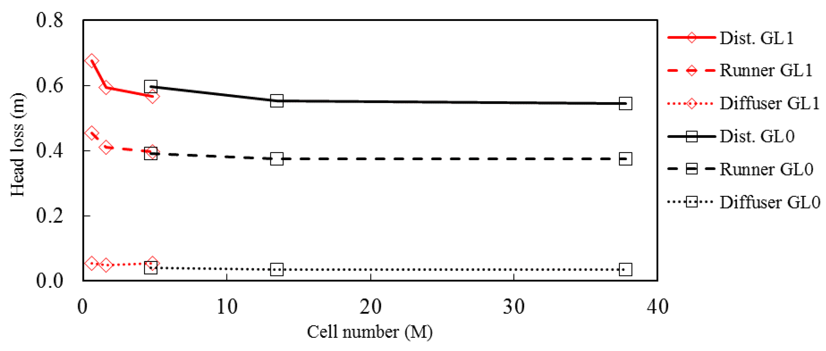
Figure 10 shows another approach to determining the independency of the solution on the mesh. Three curves represent a mesh sensitivity analysis of the distributor (upper), runner (middle), and diffuser (lower), respectively. Head loss is an important parameter of turbine performance [17]. Using this approach, head losses in the distributor, runner, and diffuser (draft tube) were estimated. The total pressure values were not significantly affected by the mesh refinement. For coarse mesh (approximately 1 million nodes), head losses in the distributor, runner, and draft tube were high. The losses are decreased with increasing the mesh density. No significant difference in the head losses was seen after a mesh refinement over 13.48 million nodes. Therefore, the authors have considered a mesh with 13.48 million nodes for their study. The mesh includes, 5.1, 6.3, and 2.08 million nodes in the distributor, runner, and draft tube, respectively. The mesh sensitivity analysis exhibited numerical errors of 1.7%, 0.6%, and 0.4% for the distributor, runner, and draft tube, respectively. The mesh sensitivity analysis exhibited numerical errors of 1.7%, 0.6%, and 0.4% for the distributor, runner, and draft tube, respectively.

Figure 10. Head losses in the turbine for the three mesh densities at two different grid levels [16]. The three curves represent a mesh sensitivity analysis of the distributor (upper); runner (middle); and diffuser (lower), respectively.

Figure 10. Head losses in the turbine for the three mesh densities at two different grid levels [16]. The three curves represent a mesh sensitivity analysis of the distributor (upper); runner (middle); and diffuser (lower), respectively.

4. Quantity of Interest

Hydraulic efficiency is an overall indicator of the turbine performance. The hydraulic efficiency reflects the average torque out from the blades, the losses in each component and effect of boundary conditions, e.g., pressure inlet or velocity inlet. Numerical estimation of hydraulic efficiency are influenced by the boundary conditions, turbulence modelling, combined performance of distributor, runner, and draft tube, interface modeling, and performance of numerical mesh under different discharge conditions. Sometimes, the numerical model performs fine at BEP and shows a small difference between the experimental and numerical values of hydraulic efficiency. However, the same model may show a difference of more than double at PL and/or HL operating conditions. Therefore, it is necessary to evaluate the performance of the mesh and selected numerical technique under different conditions.

In a high-head Francis turbine, consequences due to rotor-stator interaction and developed pressure pulsations are addressed carefully to avoid catastrophic damage. Due to the large number of blades and guide vanes, rotor-stator interaction frequency is close to the runner natural frequency and this may result in a resonance condition, sometimes. Moreover, very small vaneless gaps develop high amplitude pressure pulsations related to the rotor-stator interaction. The pressure pulsations were transmitted to the draft tube and the inlet pipe/penstock. Available numerical techniques are able to predict the rotor-stator interaction frequency but not the amplitudes. The literature on rotor-stator interaction indicate that the difference between the numerical and experimental values may reach up to 50% [24]. Therefore, it is necessary to investigate a reliable numerical technique that can predict pressure amplitudes with reduced error/uncertainty. Another challenge is the vortex breakdown occurring in the draft tube away from the best efficiency. Several numerical techniques have been applied to investigate the flow field; still, it is far from providing reliable and affordable simulations.

In a hydraulic turbine, water leaks from a gap between the rotating and stationary components. A labyrinth seal is a non-contact seal between the runner and stationary parts of the turbine. Water leaking through a labyrinth seal causes reduced turbine efficiency because the water is not utilized to generate power. The leakage flow through the seals depends on the clearance gap and operating pressure inside the turbine. Thus, the volumetric efficiency of the turbine decreases with increased leakage through the seals. The seal consists of two parts, a static seal connected to the stationary part, also known as a cover, and a rotating part connected to the runner. Both upper and lower labyrinth seals can be observed in Figure 2. At the Francis-99 workshop, various numerical studies on leakage flow through the labyrinth seals were conducted. Flow modeling in the seals is a challenging task because it requires fine meshing and significant computational power.

The following sub-sections describe results from the applied numerical techniques and their comparison experimental measurements of the efficiency, pressure, and velocity. The numerical investigation of seals is also presented.

4.1. Efficiency

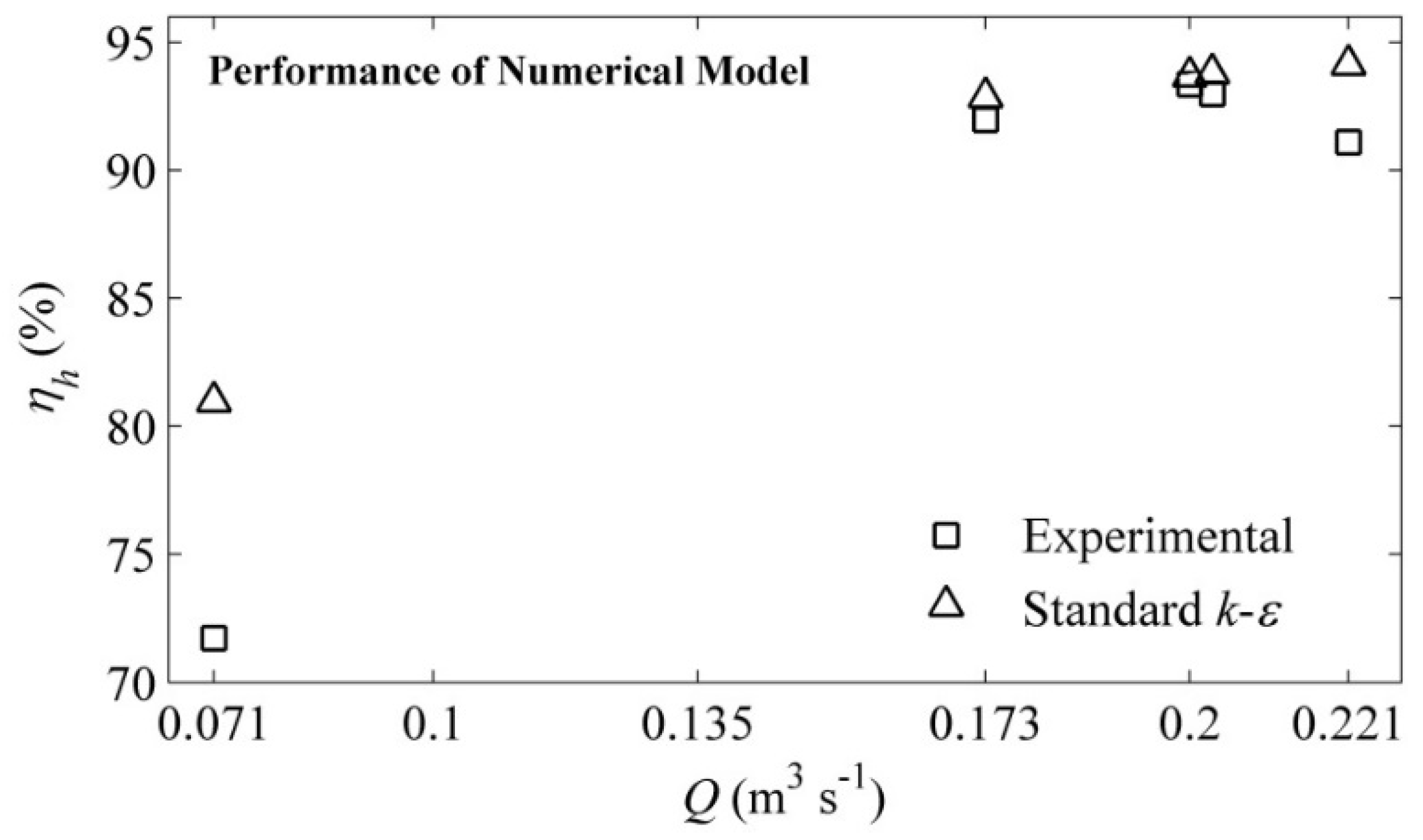
The hydraulic efficiency under PL, BEP, and HL operating conditions was numerically determined and compared with the provided experimental data. Before publishing the mesh, simulations under PL, BEP, and HL conditions were performed. Figure 11 shows the performance of the mesh provided to the researchers. Various simulations were conducted at five operating points, including the three operating points of the Francis-99 workshop. The complete turbine was simulated, starting from the spiral casing inlet to the draft tube outlet. The simulations were performed using a standard k-ε turbulence model, high-resolution advection scheme, and second-order backward Euler scheme [5]. The model demonstrated good agreement with the experimental data, and the mesh with 12 million nodes was considered to be sufficient for the workshop. The maximum difference between the experimental and numerical efficiencies was observed under PL (Q = 0.07 m³·s⁻¹, α = 3.91°) operating condition. The numerical hydraulic efficiency was 11.44% higher than the experimental efficiency. The lowest difference between the experimental and numerical results was 0.85% at the BEP (Q = 0.20 m³·s⁻¹ and α = 9.84°). The difference between the experimental and numerical efficiencies at HL (Q = 0.22 m³·s⁻¹, α = 12.44°) was 2.87%. During the simulation, flow leakage losses and other losses that occur during the measurements were not considered. Therefore, the hydraulic efficiency was over-predicted at all operating points.

Figure 11. Comparison of experimental and numerical hydraulic efficiencies at five operating points [5].

Figure 11. Comparison of experimental and numerical hydraulic efficiencies at five operating points [5].

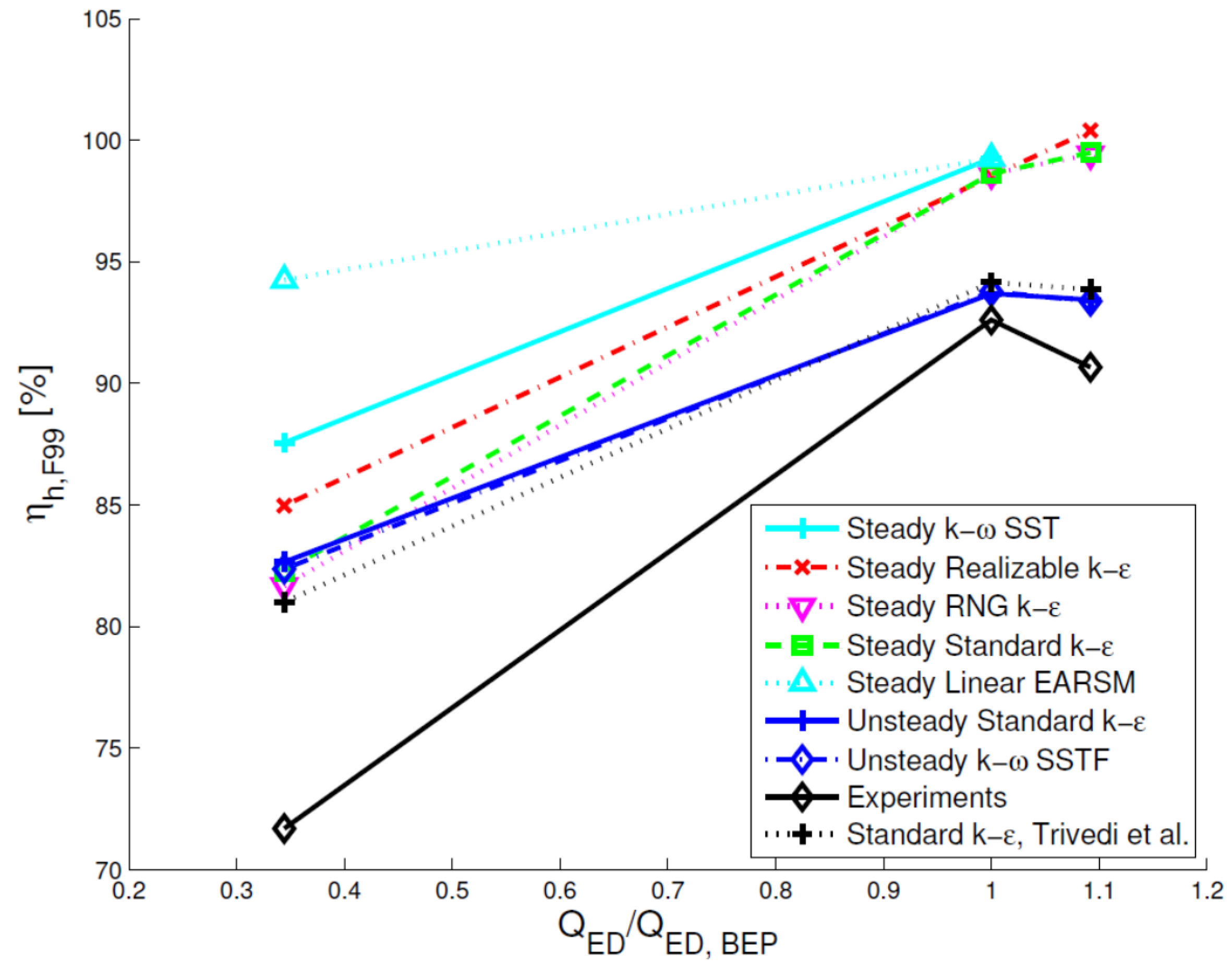
Certain researchers performed detailed numerical simulations using the provided mesh and estimated the performance with different flow modeling techniques. Figure 12 shows a comparison of the experimental and numerical values of the hydraulic efficiencies under PL, BEP, and HL conditions [15]. Both steady-state and unsteady simulations with the standard k-ε model show similar hydraulic efficiencies at PL; however at BEP and HL, the difference increases, and the hydraulic efficiency in the unsteady simulations shows a smaller difference. The realizable k-ε model shows larger differences than does the standard k-ε model. The unsteady k-ω model shows a smaller difference than does the steady-state k-ω model. Thus, the numerical results are affected by the type of simulation. One may not solely rely on steady state analysis and it may not be sufficient to understand the average flow condition in the turbine. Unsteady analysis provides information with runner angular movement with time and can chose time-averaging over certain rotation of the runner.

Figure 12. Comparison of experimental and numerical values of hydraulic efficiency under part-load, BEP, and high-load operating conditions [15].

Figure 12. Comparison of experimental and numerical values of hydraulic efficiency under part-load, BEP, and high-load operating conditions [15].

The performance of different numerical models used to investigate the Francis turbine is shown in Table 4 for all three operating points, namely, PL, BEP, and HL. The turbulence modes predicted the efficiency well under BEP and HL conditions. The challenge was to model the flow field under the PL condition. The RSM, SST, and ZLES models find small differences under the PL condition; however, the SST and ZLES models require fine meshes, which increase the computational costs. The RSM model obtains a reasonable tradeoff between computational power and numerical accuracy. For the computation of the overall turbine performance, application of RANS models may be reasonable, but these models are incapable of resolving the flow unsteadiness in the draft tube [11]. Both steady and unsteady simulations were conducted. Second order backward Euler scheme was used for the unsteady simulations. The time step size was equivalent to 0.4–2 degree of the runner revolution. The total time was equivalent to 5 to 120 revolutions of the runner. The number of runner revolutions should be sufficient to produce periodic behavior of the pressure and velocity at the runner inlet and outlet. It was observed that a minimum of five complete revolutions of the runner are usually required to attain periodic behavior at the BEP.

Hydraulic efficiency may sometimes be misleading [7] because it is an integral value and does not provide any detailed information about the performance of each component or flow details. Based on the results presented at the workshop, the differences in quantities, such as head, discharge, and torque were greater than the differences in hydraulic efficiency under the corresponding operating conditions compared to the experimental data. The torque and head values were over-predicted by 13.9% and 19.5% at the BEP, respectively [12]. The hydraulic efficiency showed a difference of −3.9% (see Table 4). Similarly, at PL, the torque, head, and the hydraulic efficiency were over-predicted by 28%, 14.1%, and 8.7%, respectively, compared to the corresponding experimental values.

Table 4. Difference in hydraulic efficiency (η) of the numerical model at BEP, HL, and PL with corresponding experimental values; $\eta =\left({\eta }_{num}-{\eta }_{\exp }\right)$. SST-shear stress transport, RSM-Reynolds stress model, ZLES-zonal large eddy simulation, BC-boundary condition, and TE-turbulence intensity.

Reference	Turbulence Model	Inlet BC	Simulation	BEP	HL	PL
[6]	Standard k-ε	Mass flow	Unsteady	2.1	--	--
[20]	Realizable k-ε	Velocity, TE = 5%	Unsteady	−0.6	1.6	9.7
[21]	SST	Mass flow	Unsteady	1.1	3.6	11
[9]	RSM	Velocity, TE = 5%	Unsteady	2.73	−0.1	8.9
[10]	SST	Mass flow	Steady	−0.4	−0.5	−8.9
	Standard k-ε			−0.7	−1.1	−7.1
	RSM			−0.7	−1.3	−7.6
[11]	SST	Mass flow	Unsteady	1	1	1.1
	Standard k-ε			1	1	1.1
	ZLES			1	1	0.9
[8]	SST	Pressure/Head	Steady	0.1	0.1	2
[12]	SST	Mass flow	Steady	−3.9	−3.4	8.7
[13]	SST	Velocity, TE = 5%	Steady	4.2	5.7	17.1
[14]	SST	Velocity, TE = 5%	Unsteady	1.8	3.8	10.3
[15]	Standard k-ε	Velocity, TE = 10%	Unsteady	1.2	2.7	10.7
[22]	SST	Mass flow	Steady	1.3	3.7	12.4
	Standard k-ε			0.2	2.7	11.1

Table 4. Difference in hydraulic efficiency (η) of the numerical model at BEP, HL, and PL with corresponding experimental values; $\eta =\left({\eta }_{num}-{\eta }_{\exp }\right)$. SST-shear stress transport, RSM-Reynolds stress model, ZLES-zonal large eddy simulation, BC-boundary condition, and TE-turbulence intensity.

Reference	Turbulence Model	Inlet BC	Simulation	BEP	HL	PL
[6]	Standard k-ε	Mass flow	Unsteady	2.1	--	--
[20]	Realizable k-ε	Velocity, TE = 5%	Unsteady	−0.6	1.6	9.7
[21]	SST	Mass flow	Unsteady	1.1	3.6	11
[9]	RSM	Velocity, TE = 5%	Unsteady	2.73	−0.1	8.9
[10]	SST	Mass flow	Steady	−0.4	−0.5	−8.9
	Standard k-ε			−0.7	−1.1	−7.1
	RSM			−0.7	−1.3	−7.6
[11]	SST	Mass flow	Unsteady	1	1	1.1
	Standard k-ε			1	1	1.1
	ZLES			1	1	0.9
[8]	SST	Pressure/Head	Steady	0.1	0.1	2
[12]	SST	Mass flow	Steady	−3.9	−3.4	8.7
[13]	SST	Velocity, TE = 5%	Steady	4.2	5.7	17.1
[14]	SST	Velocity, TE = 5%	Unsteady	1.8	3.8	10.3
[15]	Standard k-ε	Velocity, TE = 10%	Unsteady	1.2	2.7	10.7
[22]	SST	Mass flow	Steady	1.3	3.7	12.4
	Standard k-ε			0.2	2.7	11.1

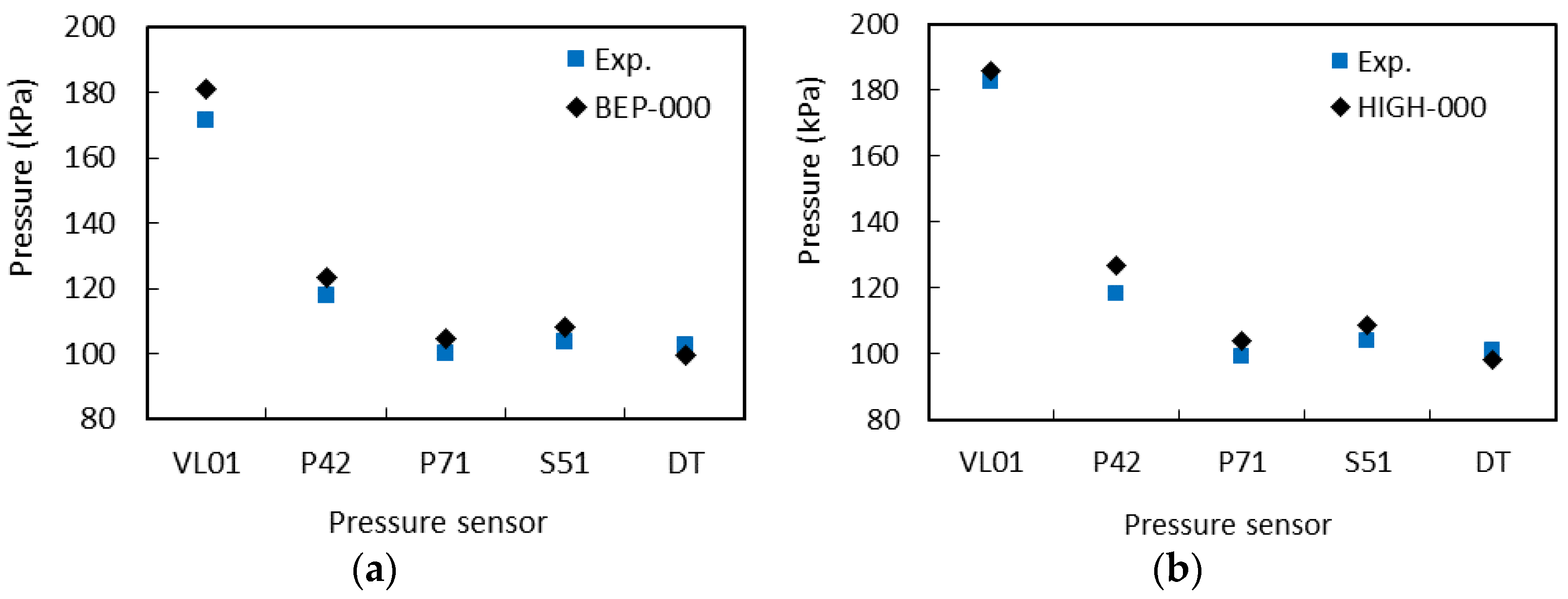
4.2. Pressure

The experimental pressure values were provided to the research groups to facilitate numerical validation and further investigations. The pressure values were acquired from six locations, namely, the vaneless space (VL01), blade pressure side (P42), suction side (S51), trailing edge (P71), and draft tube (DT11 and DT21); the locations are shown in Figure 2. Figure 13 shows a comparison of numerical and experimental average pressure values at five locations of the turbine. Two operating conditions are shown: BEP and HL. 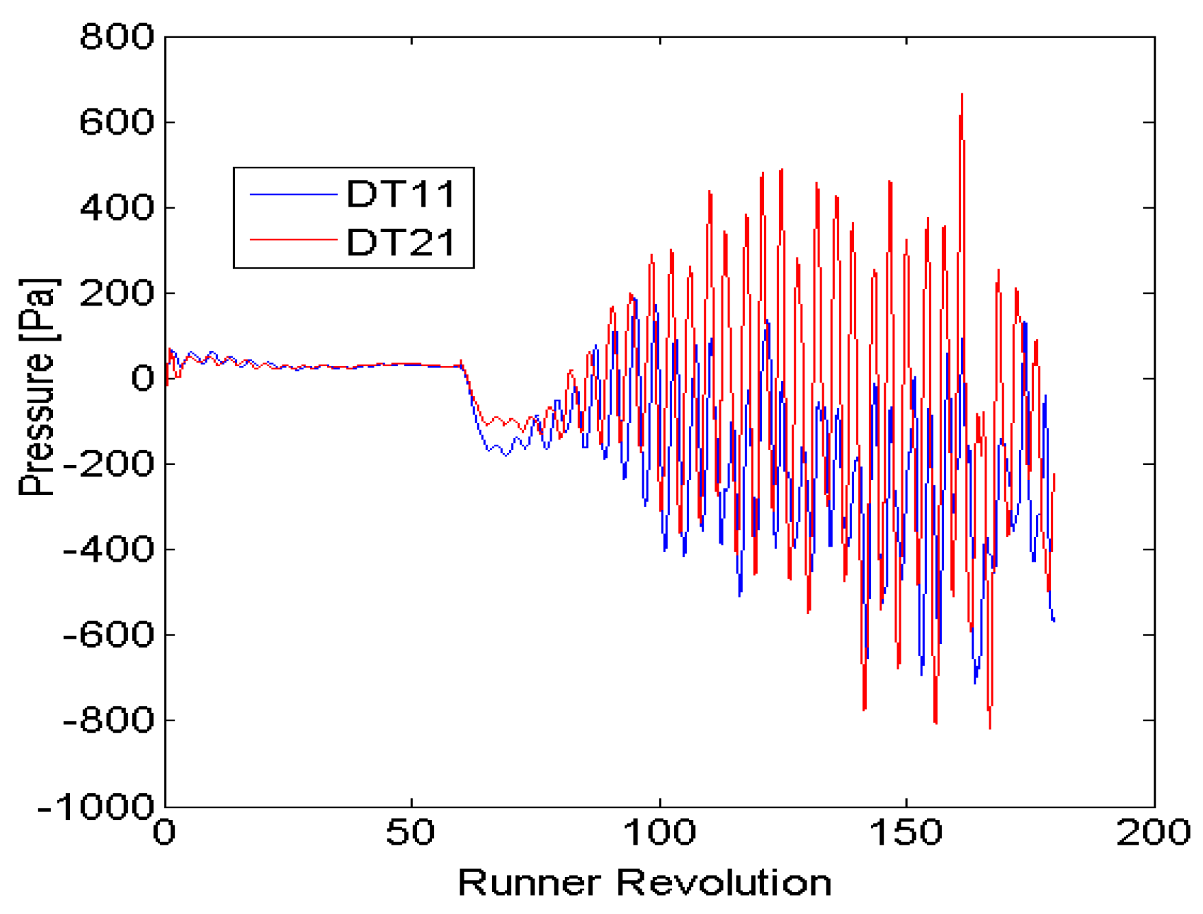The simulations were performed using the Spalart-Allmaras turbulence model [16]. A guide vane and a runner passage with a complete draft tube were modeled. At the BEP, the maximum difference between the average experimental and numerical pressure values is approximately 5.5% at VL01. At HL, the maximum difference is approximately 7.5% at location P42. In the draft tube, the same pressure difference under both operating conditions is observed. The results indicate that the average pressure might not be considerably influenced by the mesh density, discretization scheme, or turbulence model. One may use RANS models with extended wall functions and relatively coarse mesh for the expansion layer. The turbulence resolution is not significant. However, it is very well known that the RANS models have certain limitations in capturing the unsteady flow phenomena over URANS models [6]. Comparison of both the modelling approaches is shown in Figure 14. The figure shows unsteady pressure variations at draft tube locations DT11 and DT21 under the PL operating condition. A comparison between k-ω-based SST and hybrid SAS-SST models is provided. The simulation was started with the SST model, i.e., the runner revolution was from 0 to 60. No pressure pulsations are generated by the flow unsteadiness, and the variation is almost negligible; however, the y⁺ value was less than one for the SST model [19]. Then, the turbulence model was switched to the SAS-SST, and the runner revolution was from 61 to 180. The SST model was unable to capture the unsteady pressure pulsations in the draft tube as captured by the SAS-SST model. The SST model shows steady-state behavior, although the model is known to capture the unsteady flow behavior [19].

Figure 13. Average pressure loading in the model Francis turbine under BEP (a) and HL (b) operating conditions [16].

Figure 13. Average pressure loading in the model Francis turbine under BEP (a) and HL (b) operating conditions [16].

Figure 14. Comparison SST and SAS-SST turbulence models used to simulate the draft tube flow; runner revolution from 0 to 60 corresponds to SST model, and from 61 to 180 corresponds to SAS-SST model; DT11 and DT21 are the numerical monitoring points under part load operating conditions and correspond to the pressure sensor locations [6].

Figure 14. Comparison SST and SAS-SST turbulence models used to simulate the draft tube flow; runner revolution from 0 to 60 corresponds to SST model, and from 61 to 180 corresponds to SAS-SST model; DT11 and DT21 are the numerical monitoring points under part load operating conditions and correspond to the pressure sensor locations [6].

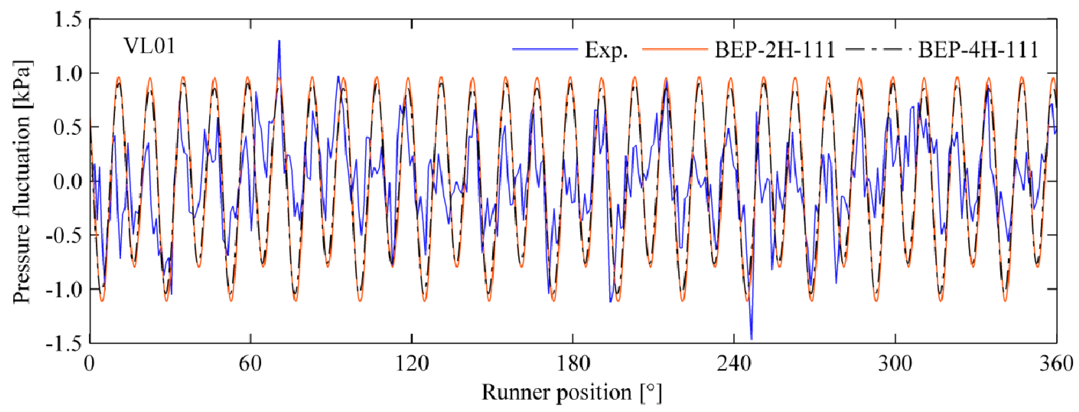
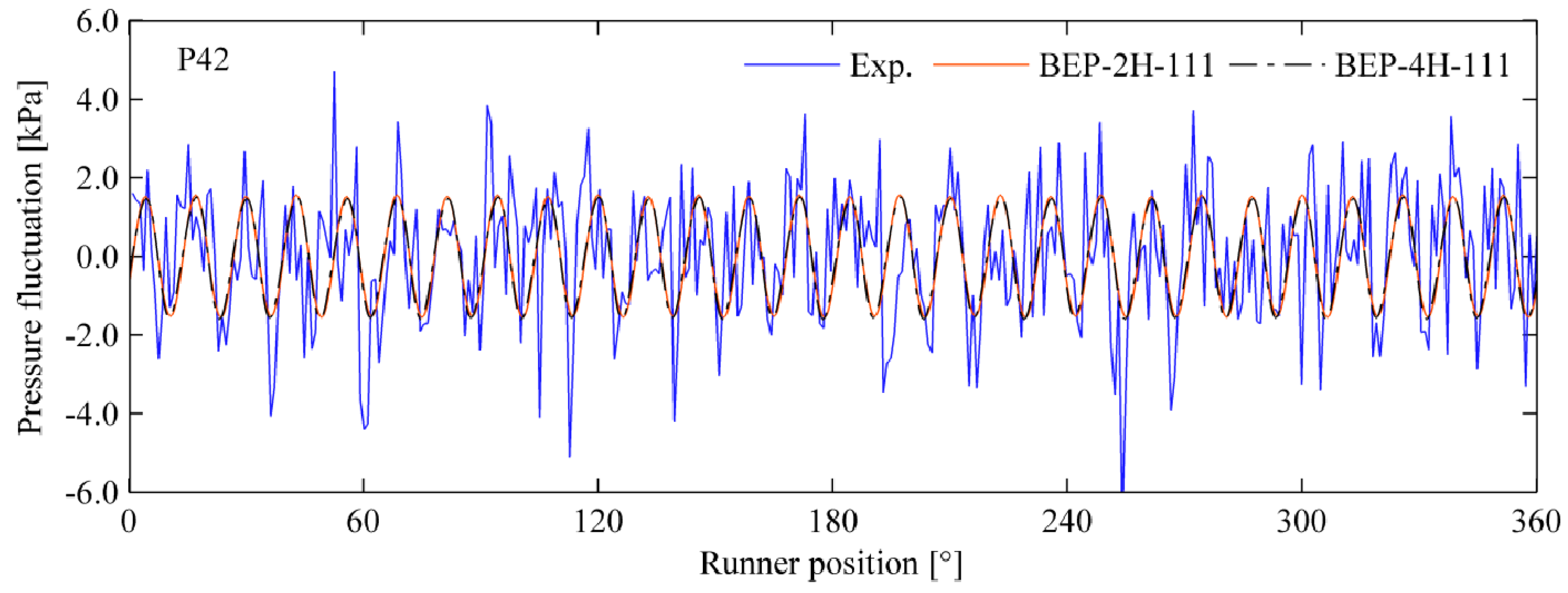
Other researchers have presented unsteady pressure pulsations at the vaneless space and runner locations. A time-domain comparison of the pressure values was conducted. Figure 15 and Figure 16 show time and pressure variations in the vaneless space and the runner at the BEP, respectively [16]. The pressure varying with the runner rotation is shown. Pressure pulsations at location VL01 correspond to the blade passing frequency of 165.6 Hz, and pressure pulsations in the runner correspond to the guide vane passing frequency of 154.5 Hz. At VL01, a good agreement between the experimental and numerical values of the pressure amplitude is observed. The selected turbulence model, Spalart-Allmaras, was able to capture the unsteady pressure pulsations in the vaneless space and the runner. Pressure amplitudes at location P42 were almost two times the amplitude of VL01. A passage modeling approach was selected for the numerical simulation. A non-linear harmonic technique was applied for the simulation and this technique is explained in Section 5, including their advantages and limitations.

Figure 15. Instantaneous pressure variation in the vaneless space at the BEP [16].

Figure 15. Instantaneous pressure variation in the vaneless space at the BEP [16].

Figure 16. Instantaneous pressure variation on the blade pressure side at the BEP [16].

Figure 16. Instantaneous pressure variation on the blade pressure side at the BEP [16].

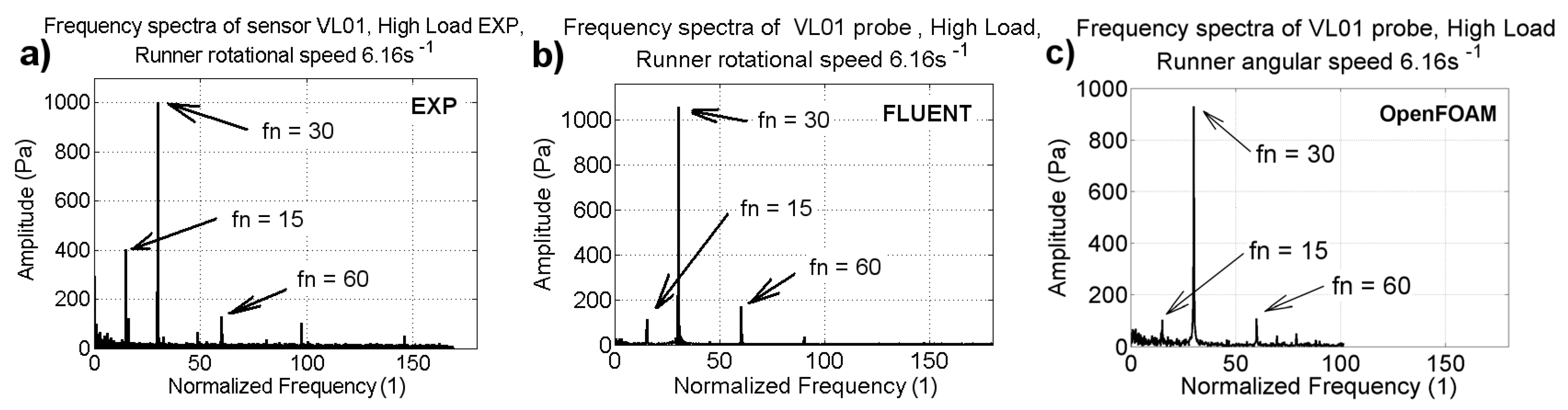
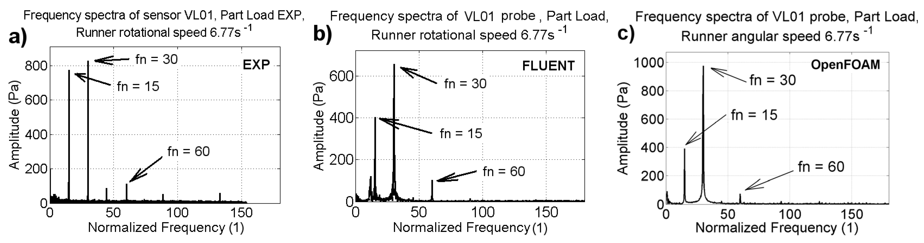
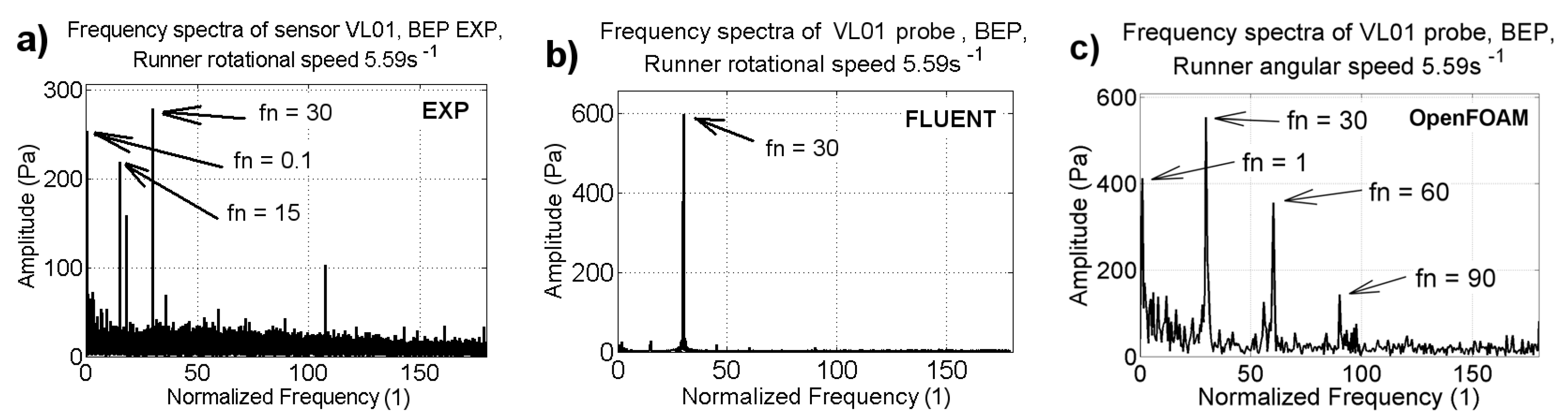
Spectral analysis and the obtained amplitude spectra at the three operating points, PL, BEP, and PL, are shown in Figure 17, Figure 18 and Figure 19 [20]. A comparison of two difference codes, FLUENT and OpenFOAM, with the provided experimental data is conducted. The frequencies are normalized to the runner speed (n) at the corresponding operating point. The dimensionless frequency of 30 corresponds to the blade passing frequency observed in the vaneless space. At PL, the results obtained with FLUENT indicate an amplitude of 0.6 kPa, and those of OpenFOAM indicate a nearly 1 kPa amplitude for a blade passing frequency of 30. The amplitudes are underestimated (15%) by FLUENT and overestimated (22%) by OpenFOAM. Both solvers underestimated the harmonic frequency of 15 by 50%. At BEP, both solvers show differences of less than 10%; however, compared to the experimental value, the amplitude of the blade passing frequency is overestimated by 50%. Under HL conditions, both solvers show similar variations in the amplitude of the blade passing frequency. OpenFOAM shows variations close to the experimental value, whereas FLUENT shows variations that are 6% higher than the experimental value. The maximum difference between the experimental and numerical values is observed for the unsteady pressure amplitude. Thus, the pressure amplitudes were found to be sensitive to the mesh density, time step sizing, turbulence modeling, discretization order, and boundary conditions [6,8,9,11,13,16,20].

Figure 17. Comparison of pressure amplitudes and frequencies in the vaneless space (VL01) under part load operating conditions; the dimensionless frequency of 30 corresponds to the blade passing frequency [20]. (a) Power spectra at the location VL01obtained using experimental pressure values (b) Power spectra at the location VL01 obtained using FLUENT solver (c) Power spectra at the location VL01 obtained using OpenFOAM solver.

Figure 17. Comparison of pressure amplitudes and frequencies in the vaneless space (VL01) under part load operating conditions; the dimensionless frequency of 30 corresponds to the blade passing frequency [20]. (a) Power spectra at the location VL01obtained using experimental pressure values (b) Power spectra at the location VL01 obtained using FLUENT solver (c) Power spectra at the location VL01 obtained using OpenFOAM solver.

Figure 18. Comparison of pressure amplitudes and frequencies in the vaneless space (VL01) under BEP operating conditions; the dimensionless frequency of 30 corresponds to the blade passing frequency [20]. (a) spectra at the location VL01obtained using experimental pressure values (b) Power spectra at the location VL01 obtained using FLUENT solver (c) Power spectra at the location VL01 obtained using OpenFOAM solver.

Figure 18. Comparison of pressure amplitudes and frequencies in the vaneless space (VL01) under BEP operating conditions; the dimensionless frequency of 30 corresponds to the blade passing frequency [20]. (a) spectra at the location VL01obtained using experimental pressure values (b) Power spectra at the location VL01 obtained using FLUENT solver (c) Power spectra at the location VL01 obtained using OpenFOAM solver.

Figure 19. Comparison of pressure amplitudes and frequencies in the vaneless space (VL01) under high load operating conditions; the dimensionless frequency of 30 corresponds to the blade passing frequency [20]. (a) Power spectra at the location VL01 obtained using experimental pressure values (b) Power spectra at the location VL01 obtained using FLUENT solver (c) Power spectra at the location VL01 obtained using OpenFOAM solver.

Figure 19. Comparison of pressure amplitudes and frequencies in the vaneless space (VL01) under high load operating conditions; the dimensionless frequency of 30 corresponds to the blade passing frequency [20]. (a) Power spectra at the location VL01 obtained using experimental pressure values (b) Power spectra at the location VL01 obtained using FLUENT solver (c) Power spectra at the location VL01 obtained using OpenFOAM solver.

4.3. Velocity

Both axial and tangential velocity profiles at both sections L1 and L2 were provided to facilitate numerical validation. All research groups had performed numerical studies on the draft tube, and almost all turbulence-modeling techniques were applied to investigate the draft tube flow field. Some of the numerical studies were able to capture the flow instability at off-design conditions [9,11], whereas others could not and exhibited steady-state behavior [15,20,22]. The steady-state behavior was associated with the application of steady RANS models.

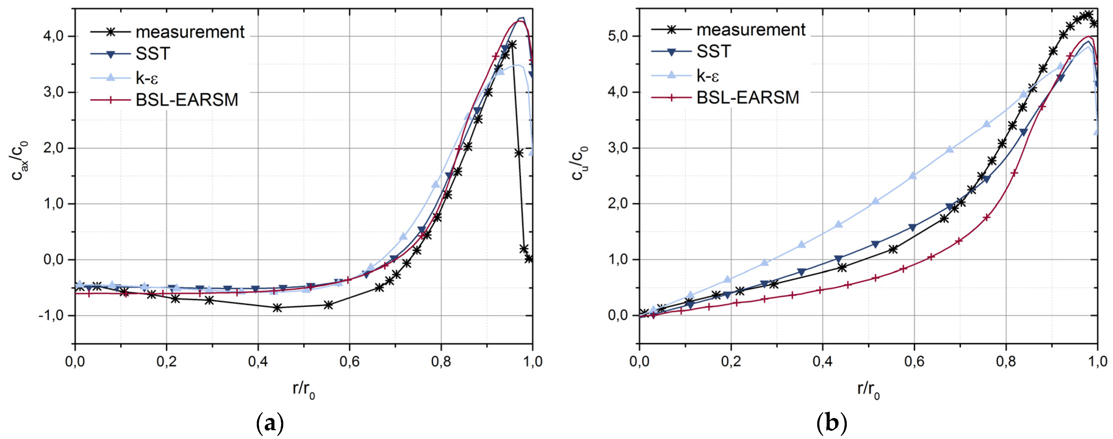
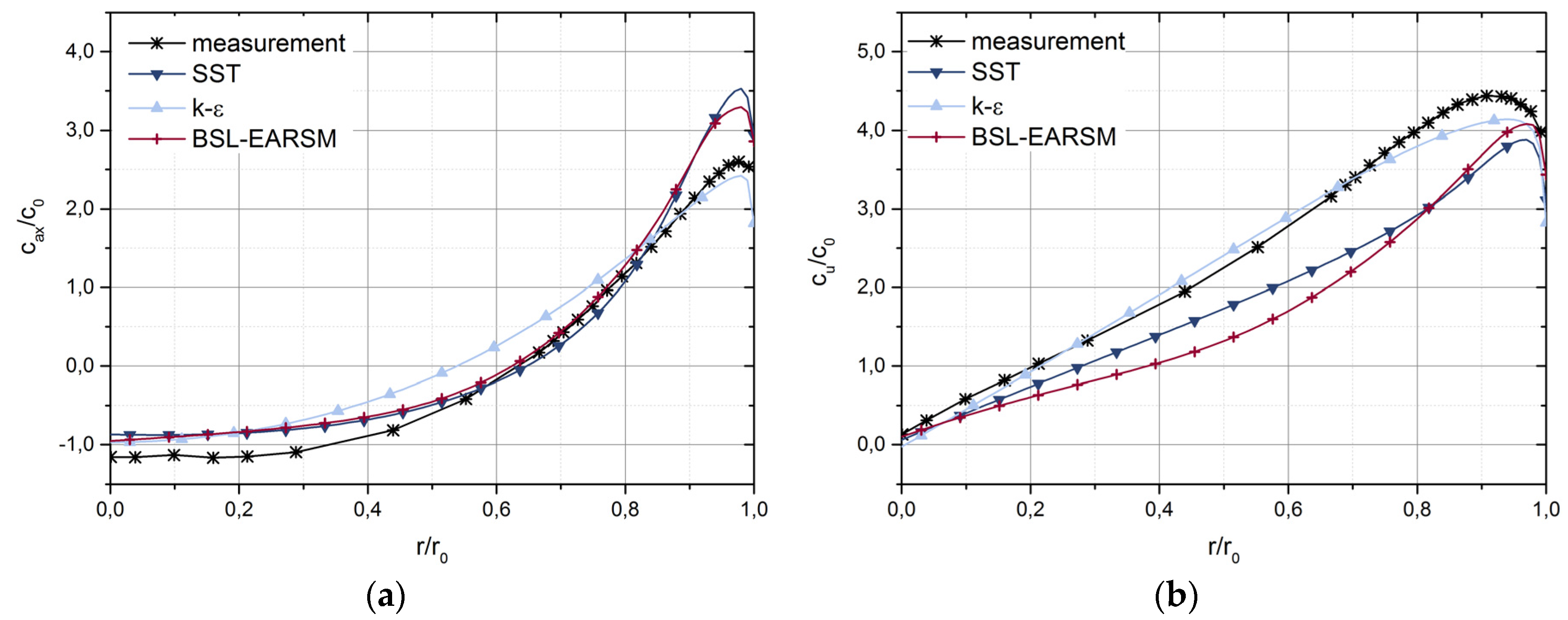
Figure 20 and Figure 21 show the average velocity at the upper (L1) and lower (L2) sections of the draft tube cone under PL operating conditions [10]. Numerical studies were conducted with three turbulence models, and the results were compared with the provided experimental data. The turbulence models follow similar trends at both sections. The SST and BSL-EARSM models show similar velocity distributions at both sections. The standard k-ε model exhibits a difficulty in capturing the velocity at both sections and large differences compared to the other two models. The two-equation RANS models often exhibit reduced accuracy for swirling flow. In this study, cavitation phenomena and flow compressibility are not considered [10].

Figure 20. Comparison of axial (c_ax) (a) and tangential (c_u) (b) velocity profiles at the upper measurement section (L1) with the experimental velocity profiles at part load [10]; c₀ is the average velocity at the measurement plane.

Figure 20. Comparison of axial (c_ax) (a) and tangential (c_u) (b) velocity profiles at the upper measurement section (L1) with the experimental velocity profiles at part load [10]; c₀ is the average velocity at the measurement plane.

Figure 21. Comparison of axial (c_ax) (a) and tangential (c_u) (b) velocity profiles at the lower measurement section (L2) with the experimental velocity profiles at part load [10]; c₀ is the average velocity at the measurement plane.

Figure 21. Comparison of axial (c_ax) (a) and tangential (c_u) (b) velocity profiles at the lower measurement section (L2) with the experimental velocity profiles at part load [10]; c₀ is the average velocity at the measurement plane.

The numerical studies using different modeling approaches have indicated that one-passage modeling and inclusion/exclusion of the spiral casing with distributor vanes do not have a significant influence on the draft tube flow [10]. Furthermore, increasing the mesh density has no effect on the axial velocity under part load operating conditions [8,11]. However, a small improvement in the velocity profile under BEP and high-load operating conditions may be observed with mesh refinement [9]. Flow modeling in a draft tube is the most challenging task and is expensive. One may simplify the draft tube flow modeling based on the flow conditions to be investigated or that are of interest. Thus, the time and effort required to model the hydraulic turbine can be reduced.

4.4. Labyrinth

To date, no results from the numerical studies on the labyrinth seals of high-head Francis turbine have been reported. At the Francis-99 workshop, three research groups [8,10,11] performed numerical studies on the labyrinth seals. Jošt et al. [11] conducted a numerical study on the labyrinth seals with three mesh densities corresponding to 10, 30, and 63 million nodes. Volumetric efficiency and losses in the seals were determined. The results for the top and bottom labyrinth seals at all three operating points are presented in Table 5. The torque losses are dependent on the discharge and the runner speed. Volumetric losses are approximately the same for all three operating points. They are, due to the small flow rate, more important at PL than at the other two operating points. Torque losses are maximized at PL mainly due to the high rotational speed. Torque losses in the upper labyrinth seal may depend on the runner rotating speed, and therefore, they are maximized at PL and minimized at the BEP. 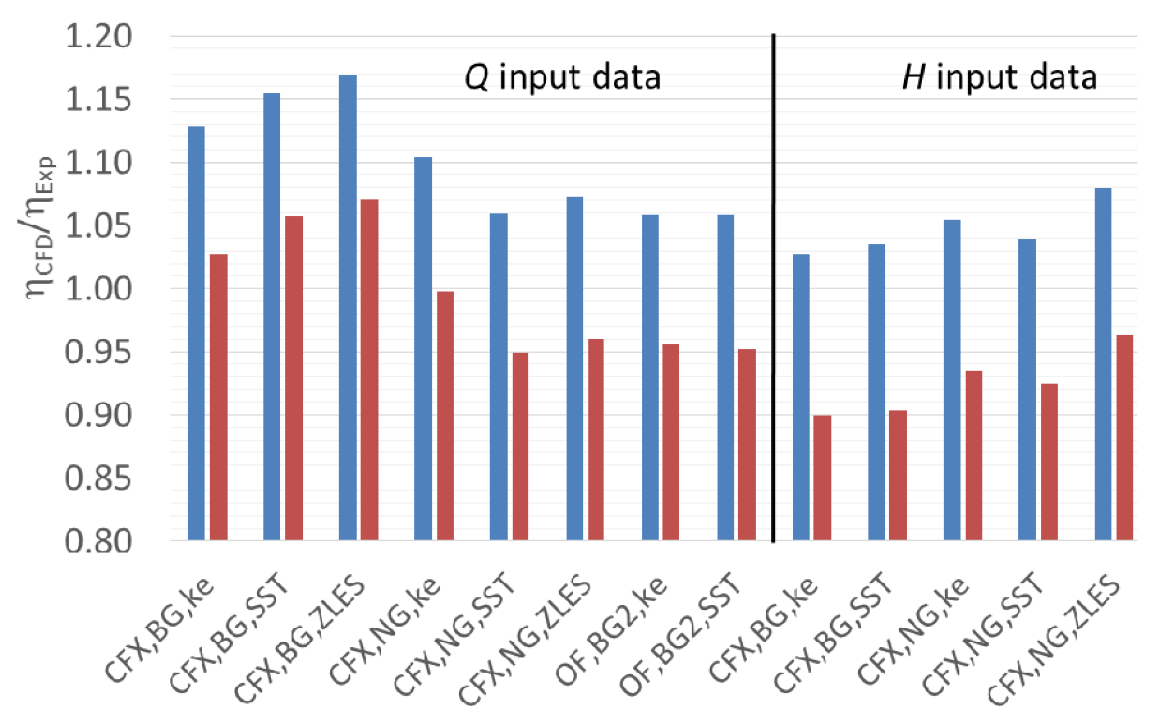Figure 22 shows the variation in hydraulic efficiency with and without losses from labyrinth seals. Comparisons of three turbulence models, SST, standard k-ε, and ZLES, using two solvers, CFX and OpenFOAM, are shown. The influence of the boundary conditions, discharge and pressure inlet on the hydraulic efficiency is also shown. Considering the losses from labyrinth seals, an improvement in the hydraulic efficiency prediction can be observed. The standard k-ε and ZLES models show small differences with the experimental value of the hydraulic efficiency. The SST model shows the maximum difference, namely, over 5%.

Table 5. Volumetric and torque losses from the labyrinth seals of the model Francis turbine under three operating conditions [11].

Operating Point	Runner Speed (Revolutions per Second)	Volumetric Losses from Lower Labyrinth Seal (lps)	Torque Losses from Lower Labyrinth Seal (Nm)	Torque Losses from Upper Labyrinth Seal (Nm)
BEP	5.59	0.43	6.1	5.35
HL	6.16	0.47	7.4	6.3
PL	6.77	0.43	8.86	7.33

Table 5. Volumetric and torque losses from the labyrinth seals of the model Francis turbine under three operating conditions [11].

Operating Point	Runner Speed (Revolutions per Second)	Volumetric Losses from Lower Labyrinth Seal (lps)	Torque Losses from Lower Labyrinth Seal (Nm)	Torque Losses from Upper Labyrinth Seal (Nm)
BEP	5.59	0.43	6.1	5.35
HL	6.16	0.47	7.4	6.3
PL	6.77	0.43	8.86	7.33

Figure 22. Determination of hydraulic efficiency with and without losses from labyrinth seals under part load operating condition for the model Francis turbine [11]; NG-new grid with approximately 14 million nodes, BG-basic grid with approximately 12 million nodes, OF-OpenFOAM; red bars in the plot indicate the hydraulic efficiency with losses from labyrinth seals.

Figure 22. Determination of hydraulic efficiency with and without losses from labyrinth seals under part load operating condition for the model Francis turbine [11]; NG-new grid with approximately 14 million nodes, BG-basic grid with approximately 12 million nodes, OF-OpenFOAM; red bars in the plot indicate the hydraulic efficiency with losses from labyrinth seals.

Mossinger et al. [10] conducted a numerical simulation and applied an analytical technique to estimate the losses from the labyrinth seals. A guide vane passage and a blade passage with labyrinth seals were modeled, and the simulations were performed using the SST model. The numerical hydraulic efficiency was compared with the provided experimental value. By including the seal losses, the numerical hydraulic efficiency was improved by 2.5%, 0.4%, and 0.2% under the PL, BEP, and HL operating conditions, respectively. The analytical study showed variations that were similar to those of the numerical study. It was noted that during the numerical study, the stability of the solution was a major concern and that if the seals are not under special investigation, it is sufficient to analytically consider the seal leakage.

5. Interface Modeling Techniques

Hydraulic turbines are operated from part load to full load conditions. The consequences of rotor-stator interactions are one of the key concerns for the life expectancy of high-head turbines. It is expensive to model and simulate a complete turbine to investigate the rotor-stator pressure amplitudes. A conventional approach is to model a blade and a guide vane passage. This approach has some limitations and introduces errors at the interface locations due to the averaging of the flow variables, i.e., flow unsteadiness is not resolved. The conventional passage modeling approach provides results with good accuracy when the pitch ratio between the modeled stator and rotor passage is equal to unity. The pitch ratio is the ratio of the circumferential angle/length of the modeled guide vane to the blade passage. For hydraulic turbines, the numbers of guide vanes and blades are chosen to avoid a common denominator, which may trigger instabilities in the turbine [19]. A pitch ratio equal to unity is thus difficult to obtain for numerical investigations.

Recently, a technique was developed to model the flow passages without limiting the pitch ratio [19]. A method called a Fourier transformation is used in this technique [25,26,27]. Two research groups modeled the Francis turbine using this technique and presented the results during the workshop [6,16]. 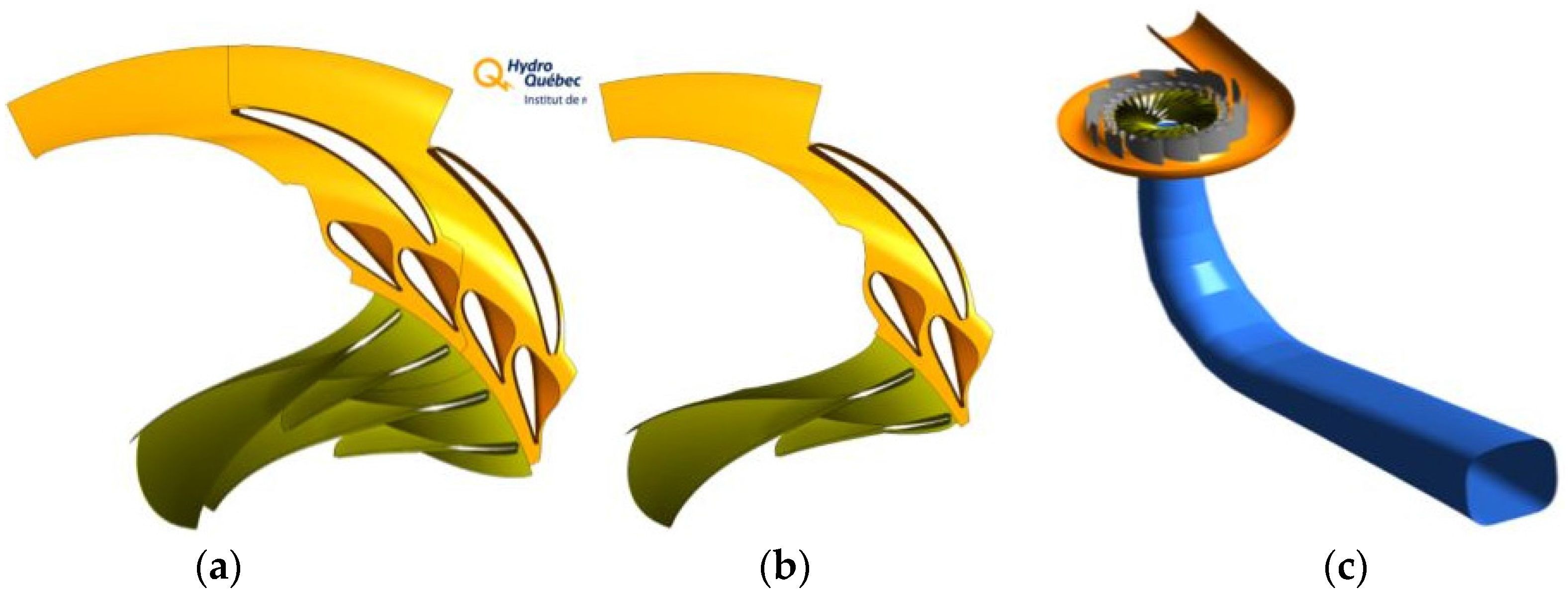A passage of the distributor and a blade with a splitter was modeled, and the performance was compared with the other approaches, i.e., profile transformation, and the complete turbine. The pitch ratio between the guide vane and blade passages was 0.933. 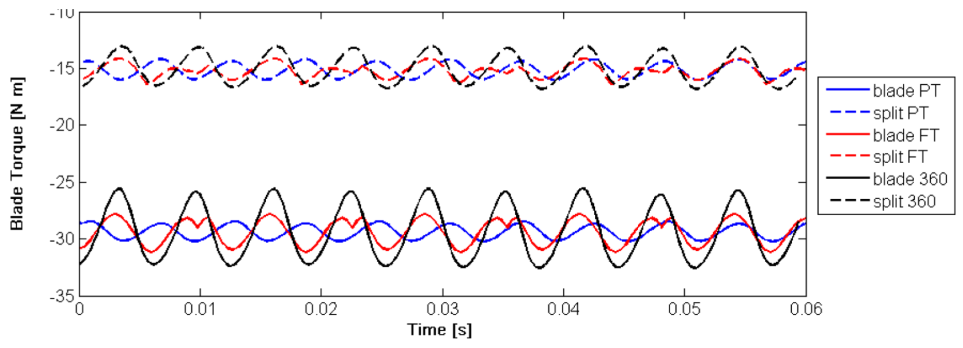Figure 23 shows three flow modeling approaches for a Francis turbine, two-passage modeling (used for the Fourier transformation), one-passage modeling (profile transformation), and complete turbine. The obtained results are shown in Figure 24. The simulations were conducted using the SST model, and the y⁺ value was less than one. The maximum amplitude of the torque was captured by the complete turbine modeling approach. The profile transform technique predicted the lowest amplitude. The Fourier transform technique showed an amplitude that was lower than that of the complete turbine modeling approach and higher than that of the profile transformation. This indicates that the Fourier transformation technique provides a better performance than does the profile transformation when the pitch ratio does not meet the requirements. This approach provides a compromise between the numerical accuracy and computational power required to simulate the complete turbine. The challenge with this approach lies in correctly estimating the amplitudes generated by the guide vanes and blade interactions. The approach often underestimates the amplitudes.

Figure 23. Comparison of flow modeling approaches applied to a Francis turbine; (a) configuration used for the Fourier transform; (b) configuration used for the profile transform; (c) configurations show the complete turbine [6].

Figure 23. Comparison of flow modeling approaches applied to a Francis turbine; (a) configuration used for the Fourier transform; (b) configuration used for the profile transform; (c) configurations show the complete turbine [6].

Figure 24. Variation in the blade and splitter torque in a model Francis turbine under the BEP operating conditions; PT-profile transform, FT-Fourier transform, 360-complete turbine modeling [6].

Figure 24. Variation in the blade and splitter torque in a model Francis turbine under the BEP operating conditions; PT-profile transform, FT-Fourier transform, 360-complete turbine modeling [6].

The implemented form of Fourier transformation technique based on Navier-Stocks equations is described below:

$$\frac{\partial U_i}{\partial x_i}=0$$

(9)

$$\frac{\partial U_i}{\partial t}+U_j\frac{\partial U_i}{\partial x_j}=-\frac{1}{\rho }\frac{\partial P}{\partial x_i}+\frac{\partial }{\partial x_i}\left(\nu \frac{\partial U_i}{\partial x_j}-{\tau }_{ij}\right)$$

(10)

The velocity is decomposed as $u_i=U_i+u_i^{\prime }$; U_i is the mean velocity component, $u_i^{\prime }$ is the fluctuating component of velocity, P is the average pressure, ν is the kinematic viscosity, and ${\tau }_{ij}=\overline{u_i^{\prime }{u}_j^{\prime }}$ are the Reynolds stresses. The decomposition of the conservative variables into the mean value $\overline{\varphi }$ and N periodic perturbations ${\varphi }^{\prime }$ with complex amplitude $\tilde{\varphi }$ is assumed:

$$\varphi \left(\stackrel{\rightharpoonup }{x},t\right)=\overline{\varphi }(\stackrel{\rightharpoonup }{x})+{\displaystyle \sum _{k=1}^N{\varphi }_k^{\prime }\left(\stackrel{\rightharpoonup }{x},t\right)}$$

(11)

$${\varphi }^{\prime }\left(\stackrel{\rightharpoonup }{x},t\right)={\tilde{\varphi }}_k(\stackrel{\rightharpoonup }{x}){\mathrm{e}}^{i{\omega }_{k}t}$$

(12)

Substituting Equation (11) into Equation (10) and time-averaging yields the mean flow equations. Considering only one perturbation and adding a pseudo time-dependence gives:

$$\frac{\partial U_i}{\partial t}+U_j\frac{\partial U_i}{\partial x_j}+\frac{\partial U_i^{\prime }{U}_j^{\prime }}{\partial x_j}=-\frac{1}{\rho }\frac{\partial P}{\partial x_i}+\frac{\partial }{\partial x_i}\left(\nu \frac{\partial U_i}{\partial x_j}-{\tau }_{ij}\right)$$

(13)

Subtracting the time-averaged flow Equation (13) from the unsteady RANS Equation (10) and keeping only the first order terms yields the transport equations required to solve the unsteady perturbations:

$$\frac{\partial U_i^{\prime }}{\partial x_i}=0$$

(14)

$$\frac{\partial U_i^{\prime }}{\partial t}=-\frac{1}{\rho }\frac{\partial P^{\prime }}{\partial x_i}+\nu \frac{{\partial }^2{U}_i^{\prime }}{\partial x_j^2}$$

(15)

The final solution can be constructed in time by computing the perturbations at a given time using Equation (12) and adding them to the time-averaged flow. This operation allows obtaining an approximation of the unsteady flow field. It should be noted that interactions between the perturbations themselves can only be achieved through their respective interaction with the mean flow by the deterministic stresses. The resolution of the perturbations equations in the frequency domain allows the usage of periodic computational domains with mixing plane interfaces, thus lowering the required memory and simulation time. Periodic boundary conditions are implemented using a simple phase shift of the complex amplitudes, which are solved for the frequencies of the perturbations coming from adjacent computational domains with different rotational speeds. Detailed explanation of this technique is available in the literature [25,26,27,28,29].

The transient blade row modeling technique is applied using a constant angular speed of the runner and uniformly sized time steps [27]. This technique may not be applied to simulate transient conditions of the turbine such as those during start-stop, total load rejection, and speed-no-load. Moreover, this technique supports two passages for each component. There must be a rotating and stationary passage. Overall, the technique and passage modeling approach is not as expensive as modeling and simulating a complete turbine. The approach of passage modeling using the Fourier transform technique provides acceptable results, although it has certain limitations.

6. Summary

Extensive numerical studies have been conducted on a high-head Francis turbine model for the first Francis-99 workshop by several participants. A large range of mesh densities, setups, flows and turbulence models were applied. The experimental results were available to the participants, thereby allowing them to fine tune their simulations. Many questions were raised during the workshop concerning the challenges related to accurate simulations of high-head Francis turbines.

Apart from the proposed mesh, many participants have created their own meshes to improve the quality. Their main focus was near-wall modeling with different approaches. Further, a quality assessment of the mesh is necessary for a proper interpretation of the numerical results. However, a mesh sensitivity analysis was not always possible due to computational limitations. Systematic information about the mesh quality parameters, minimum angle, volume change, aspect ratio, etc. is a first step but not sufficient, per se. In addition to the mesh, the numerical schemes and type of code should also be stipulated. The same mesh will not provide the same results for different codes; it is also a function of the code used, and each code operates differently.

The hydraulic efficiency obtained through different numerical techniques was deviating from −7.6% to 17.1% as compared to the corresponding experimental values. The variation is attributed to the omission of the seal leakage losses. Often, numerical results are misleading because the torque and head are over-predicted with an inlet flow boundary condition; see Lenarcic et al. [12]. Since the torque generated by the turbine and the available head are related to each other, the hydraulic efficiency is fairly well predicted. Using the head as the inlet boundary condition provides a higher flow rate, decreasing the hydraulic efficiency. The reason is an under-prediction of the viscous losses. The use of a wall function assuming equilibrium between the production and dissipation of turbulence is widely used in the simulation of hydraulic turbines. The boundary layer of hydraulic turbines is never fully developed because of the continuously changing geometry and rapid change in pressure gradients. Resolving the boundary layer up to y⁺ = 1 is not feasible, even with RANS models. There is a need to develop wall functions that enable the estimation of viscous losses under boundary development if accurate simulations are to be developed. Improved simulations and results enable reliable estimation of the blade loading.

The labyrinth seals in high-head Francis turbines may represent the losses up to 6%, especially at part load because a low flow rate is used [8]. The volumetric losses are nearly constant because they are proportional to the pressure drop across the labyrinth seals and the clearance gap. The viscous losses are a function of the runner speed. The simulation of such details is extremely expensive in terms of computational capacity. The main advantage is the simplicity of the geometry, thereby allowing high mesh quality. A detailed study has been conducted on the subject, and various relations exist to estimate the related losses. An assessment of the volumetric losses on the runner incoming flow and draft tube flow development is of interest in terms of boundary layer and loss analysis. At the Francis-99 workshop, numerical investigations on leakage flow through the labyrinth seals were conducted. The simulations were performed using 63 million nodes. The volumetric efficiency and losses in the seals were determined. It was indicated that if the seals are not under special investigation, it is sufficient to consider the seal leakage losses through analytical techniques.

In a high-head Francis turbine, pressure amplitudes generated by the rotor-stator interactions are a major concern. A recently developed flow modeling technique was applied to investigate the rotor-stator interaction in the model Francis turbines for the first time. This technique showed pressure variation and amplitudes close to the corresponding values obtained with 360 degree modelling of the runner blades and guide vanes. It provides a compromise between numerical accuracy and required computational power for simulating the complete turbine. One may consider this approach when time dependent pressure loading is required within a short period of time with limited computational capacity.

PIV measurements were conducted in the draft tube to enable a detailed comparison and validation of the numerical models. Tangential and axial velocity profiles at two sections of the draft tube cone were provided. Numerical studies conducted using RANS models showed very similar trends for the velocity distribution. The modes indicated steady-state behavior in the draft tube. It was suggested that this could be attributed to the limitations of the RANS models and large y⁺ value. The main difficulty was the accurate prediction of the flow condition close to the boundaries. Starting from two-equation eddy viscosity models and extending to hybrid models such as SAS-SST and ZLES, all of the models showed good performance at the BEP. However, the flow field under part load conditions was challenging, and all of the researchers experienced difficulty in obtaining results with good accuracy. It was concluded that the mesh distribution near the boundaries plays significant role for improving the pressure and velocity distribution in the turbine. The hybrid models provided improved results, but these models require fine meshes near the boundaries, which are more computationally expensive than the scalable wall function approach.

At the Francis-99 workshop, numerical simulations were conducted using three modeling approaches: (1) modeling of a complete turbine; (2) modeling of the components; and (3) passage modeling. The simulation of a complete turbine is more expensive than the other two approaches. No significant difference was found between the results obtained with the complete turbine and component modeling approaches. It was considered that the component modeling approach would provide the optimum solution when accurate boundary conditions are prescribed. Further, one can select a passage modeling approach and create a fine mesh near the boundaries to reduce the necessary computational power and time. This approach provides good results but does not consider the influence of the neighboring passages. However, using recently developed techniques of passage modeling can provide reliable results, including dynamic pressure loading generated by rotor-stator interaction.

To minimize the error due to the use of different mesh types and densities, it was noted that a mesh with a uniform density would be provided. The simulations would be conducted using the provided mesh only and validated with the provided experimental data. The mesh would be provided with different y⁺ values, namely, y⁺ < 1 and 11 < y⁺ < 300, to accommodate different turbulence models. At the second Francis-99 workshop, both steady-state and transient operating conditions will be investigated. Numerical models will be validated with the steady-state experimental results, and the same model will be used for transient conditions. Load variations and start-stop conditions will be investigated under transient operations. The primary focus will be development of numerical technique and detailed flow investigation of the hydraulic turbine during the transient conditions.