Joint Estimation of the Electric Vehicle Power Battery State of Charge Based on the Least Squares Method and the Kalman Filter Algorithm

Abstract

An estimation of the power battery state of charge (SOC) is related to the energy management, the battery cycle life and the use cost of electric vehicles. When a lithium-ion power battery is used in an electric vehicle, the SOC displays a very strong time-dependent nonlinearity under the influence of random factors, such as the working conditions and the environment. Hence, research on estimating the SOC of a power battery for an electric vehicle is of great theoretical significance and application value. In this paper, according to the dynamic response of the power battery terminal voltage during a discharging process, the second-order RC circuit is first used as the equivalent model of the power battery. Subsequently, on the basis of this model, the least squares method (LS) with a forgetting factor and the adaptive unscented Kalman filter (AUKF) algorithm are used jointly in the estimation of the power battery SOC. Simulation experiments show that the joint estimation algorithm proposed in this paper has higher precision and convergence of the initial value error than a single AUKF algorithm.

1. Introduction

In an electric vehicle, the power battery State of Charge (SOC), an important parameter of the battery state, is used to directly reflect the remaining capacity of the battery and provide a basis for the formulation of an optimal energy management strategy for the vehicle control system. An inaccurate SOC will result in a reduced performance of the vehicle and lead to potential damage to the battery system; therefore, it is critical to develop algorithms that can accurately estimate the battery SOC in real time.

An accurate estimation of the SOC is important to prolong the battery life and improve the performance of the electric vehicle [1,2]. However, because the battery is a strongly nonlinear and time-variable system, in practical applications it is hard to measure the SOC directly due to its complicated electrochemical processes and the influence of various factors [3]. At present, the most common methods of estimation [4,5,6,7,8] can be roughly divided into two main categories.

One main category is based on the relationship between energy conservation and the physical properties of the battery. For example, the most commonly used methods in this category include the open circuit voltage method and the ampere-hour integral method, among others, in which the battery charge and discharge current or the open circuit voltage are used to calculate the residual capacity of the battery.

The open circuit voltage method, when used alone, can only be applied to an electric vehicle in a non-moving state. It cannot provide a real time dynamic estimation and is therefore usually used to provide a rough SOC initial value for other methods.

The ampere-hour integral method calculates the accumulated charge of the battery during charging or discharging and among other advantages, it is economical and easy to conduct. However, when it is applied in electric vehicles, the following main problems result: (1) the SOC initial value must be obtained by other methods; (2) a higher current measurement accuracy is needed, because the accuracy of the SOC estimation is largely determined by the current measurement accuracy; and (3) the accumulative errors cannot be eliminated, and as the charging or discharging time increase, the accumulative errors may get out of control.

Another main category of methods for SOC estimation is by first establishing a mathematical model of the battery, and then the battery SOC can be estimated indirectly based on the established model, the measured charge or the discharge current, and the terminal voltage. Common methods in this category include the neural network and the Kalman filter (KF) methods, among others.

The neural network method utilizes a complex nonlinear system, i.e., a neural network, which is composed of a large number of simple neurons with extensive connections. The neural network can automatically induce, organize and study the collected data to obtain the inner rules of these data. The neural network also has the ability to map a nonlinear system and thus can better reflect the dynamic characteristics of a battery. The disadvantage of the neural network method is that a large amount of data is needed for training, and the SOC estimation accuracy is greatly influenced by the training methods and the training data.

The main idea behind the Kalman filter method is to make an optimal estimation of the minimum mean square sense of the dynamic system states. This method has strong error correction ability and requires a highly accurate battery model. When the KF method is used to estimate the SOC, the general mathematical form of the battery model can be expressed as:

$$\mathrm{State}\mathrm{equation}:x_{k+1}=A_x{x}_k+B_k{u}_k+w_k$$

(1)

$$\mathrm{Observation}\mathrm{equation}:y_k=C_k{x}_k+D_k{u}_k+v_k$$

(2)

where u_k is the input of the system, including the battery current, residual capacity, battery temperature, among other variables, and y_k is the output of the system, which usually indicates the terminal voltage of the battery. The most difficult challenge of the KF method is determining the state equation and the observation equation.

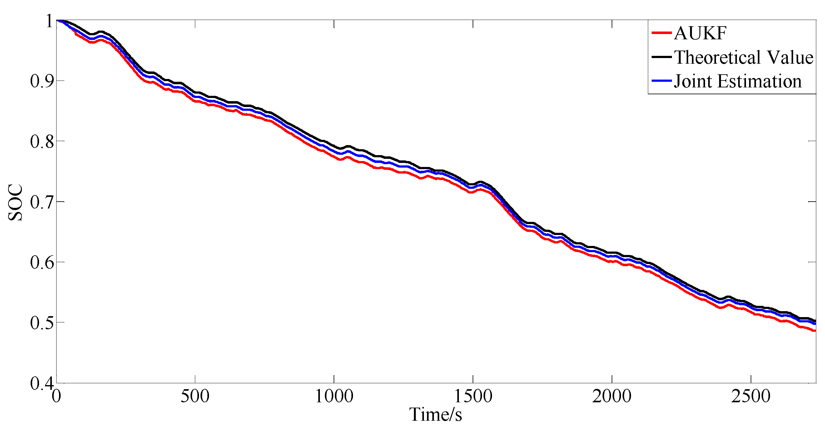
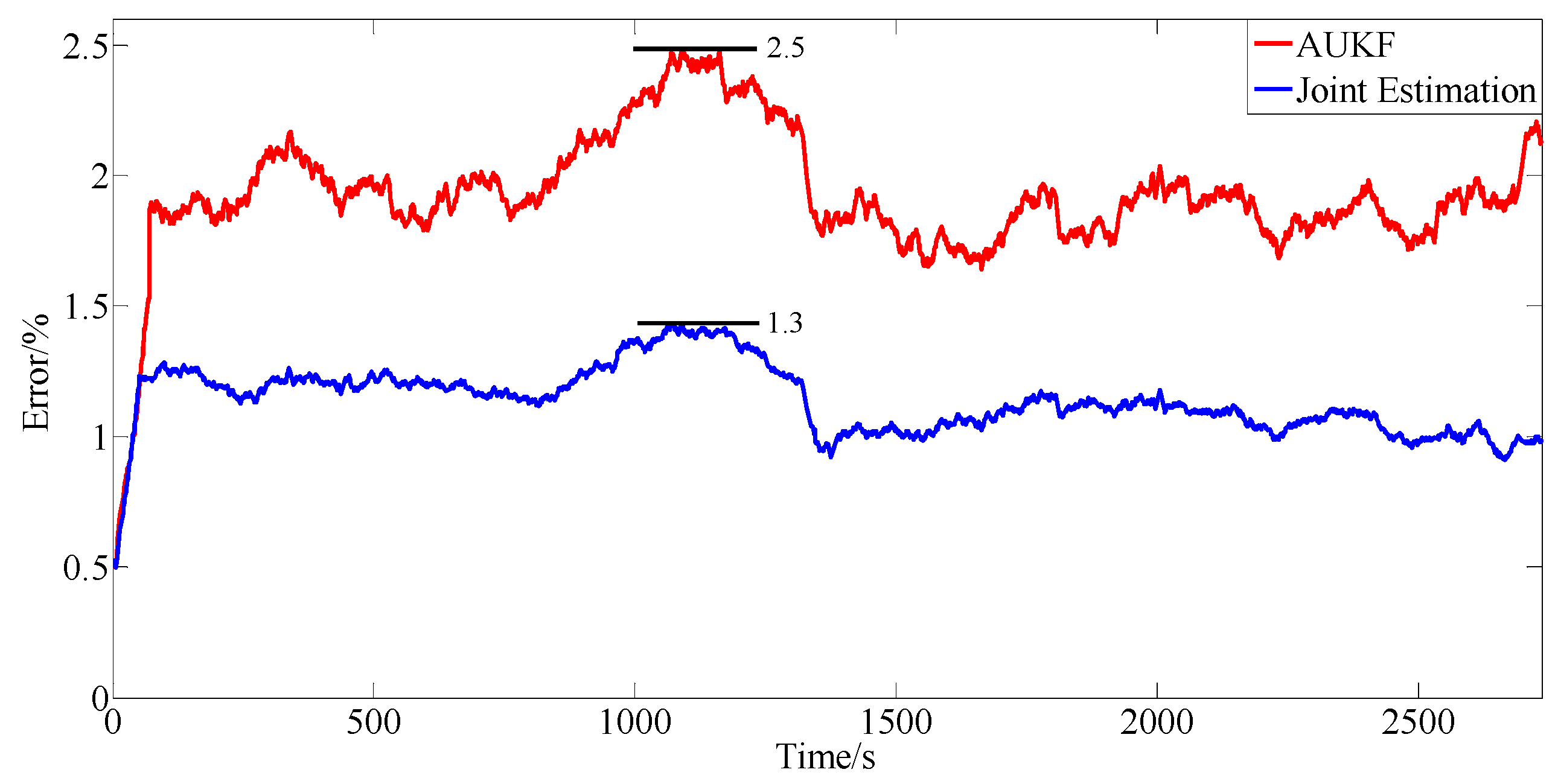
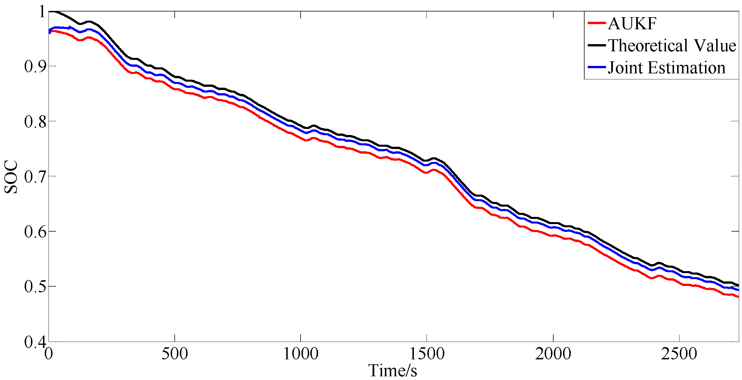
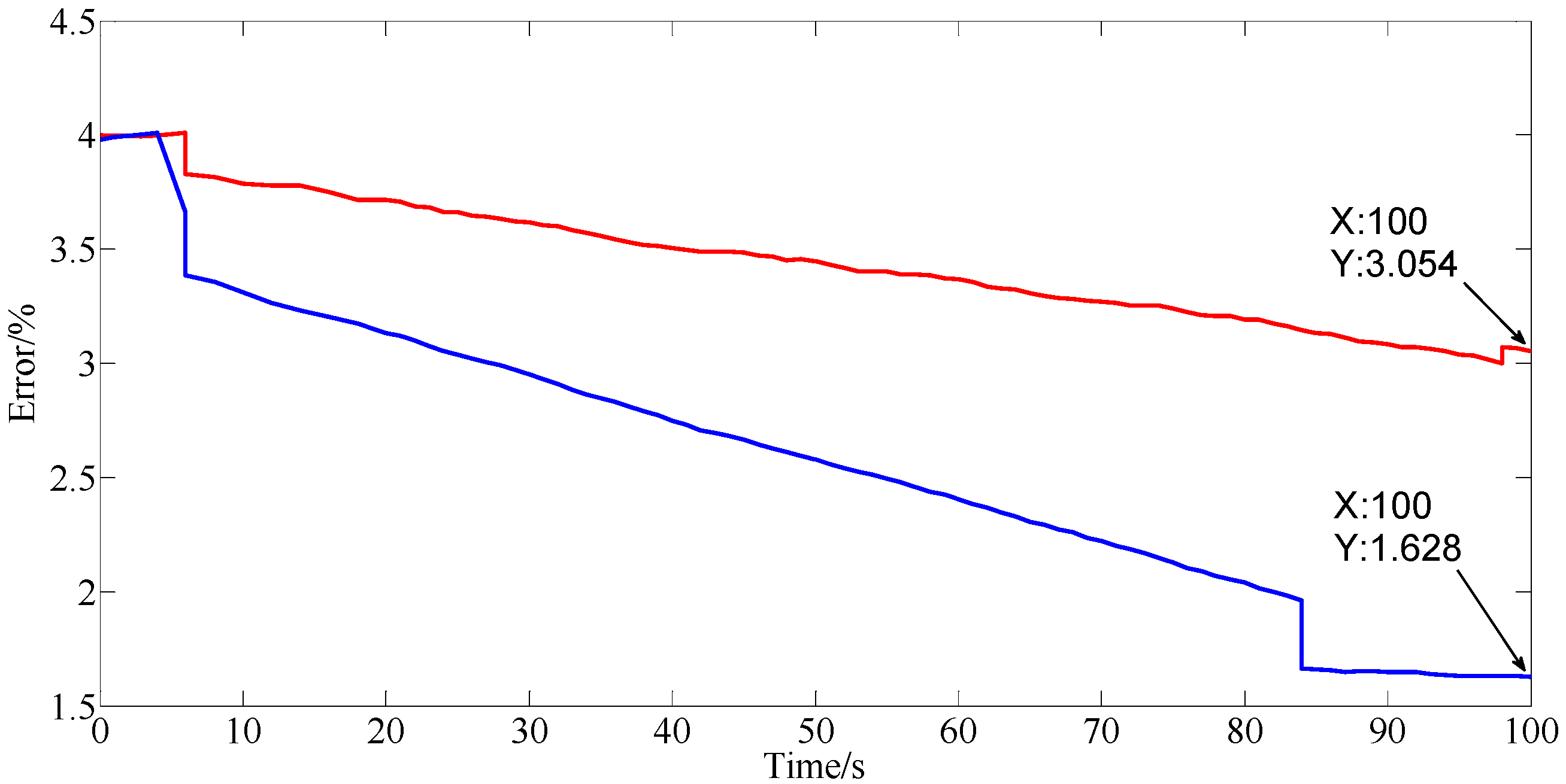
In this paper, using the second–order RC circuit as the equivalent model of the power battery, the online parameters of the circuit model are identified and the SOC is estimated based on the least squarea (LS) method with a forgetting factor and adaptive unscented Kalman filtering (AUKF). The comparison of these two algorithms is given, and a novel joint estimation algorithm of the power battery SOC based on the LS and the KF is proposed. The joint algorithm has the characteristics of a high estimation precision and good convergence to the initial value error. Furthermore, the advantages of the proposed algorithm are demonstrated by simulation experiments.

The structure of this paper is arranged as follows: in Section 1, the most commonly used methods for SOC estimation are introduced, and the proposed method of this paper is briefly described. In Section 2, the proposed equivalent circuit structure is determined. Dynamic parameter identification and model verification of battery model are described in Section 3. In Section 4, the AUKF algorithm is presented. In Section 5, using the LS with a forgetting factor and the AUKF algorithm to jointly estimate the power battery SOC, the advantages of the proposed algorithm is demonstrated by simulation experiments. Finally, in Section 6, the research results of this paper are summarized, and future research directions are provided.

2. Building the Battery Model

Generally, a good battery model provides an accurate description of the dynamic and static characteristics of the battery, has a relatively simple model structure making analysis and calculations easy and is not difficult to implement for a project. Currently, four main equivalent circuit models, i.e., the Rint model, Thevenin model, PNGV model, and a multi-order RC circuit model, are widely used in electric vehicle simulation [9,10,11,12,13].

The first three models have simple structures but low precision performances. In the multi-order RC circuit model, as the model order increases, the model precision will increase. However, with increasing model order, the model will not be pragmatic due to its computational complexity.

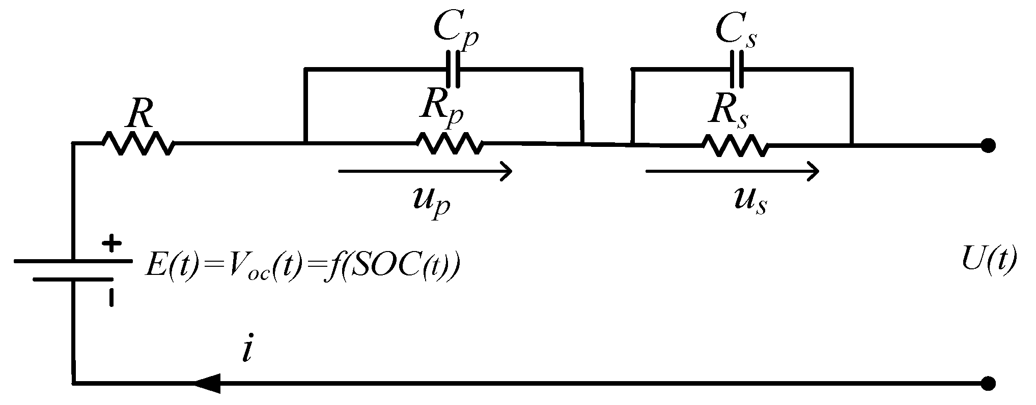
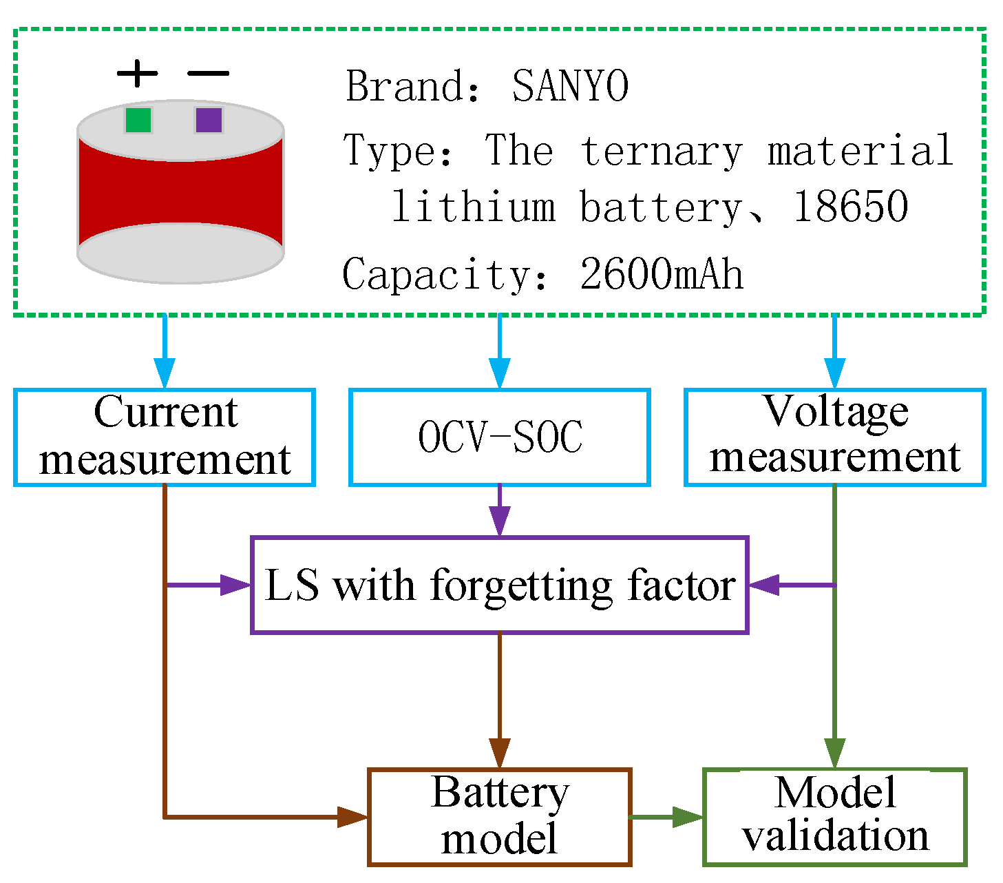
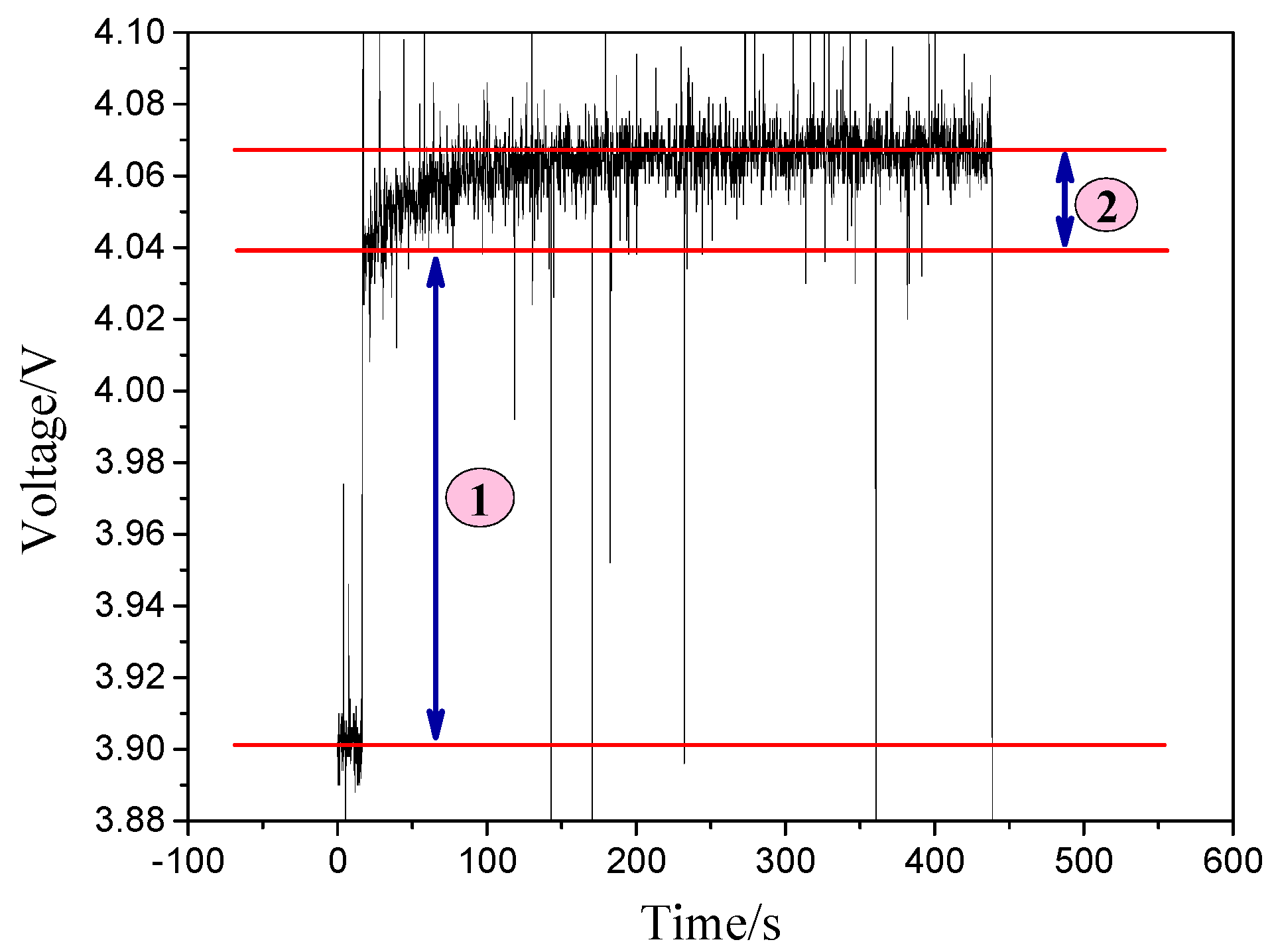
Thus, this article uses the second-order RC equivalent circuit as the battery model, as shown in Figure 1. Figure 2 shows the terminal voltage response of a 2.6 Ah Sanyo ternary lithium battery after completing a discharge cycle.

Figure 1. The second-order RC equivalent circuit.

Figure 1. The second-order RC equivalent circuit.

Figure 2. The terminal voltage response after the completing a discharge cycle.

Figure 2. The terminal voltage response after the completing a discharge cycle.

This model includes three parts:

• Voltage source: Using the open circuit voltage V_oc as the power battery electromotive force, this work neglects the temperature and SOH influences on the open circuit voltage (OCV) and only studies the relationship between V_oc and the battery SOC at a constant temperature (25 °C) and constant SOH (i.e., a new battery).
• Ohmic resistance: The battery’s resistance consists of electrode materials, electrolytes and other resistors. The change in voltage in region ① in Figure 2 is due to the influence of the ohmic resistance R.
• RC loop circuit: Two links of a resistor and a capacitor superpose to simulate battery polarization [14], which is used to simulate the process voltage stabilization after discharge. The region ② of Figure 2 shows the change in voltage influenced by the RC loop circuit.

Equation (3) shows the function relation of the equivalent circuit model in Figure 1:

$$\{\begin{array}{c}E\left(t\right)=iR+u_s+u_p+U\left(t\right)=F\left(SOC\left(t\right)\right)\\ i=\frac{u_s}{R_s}+C_s\frac{d{u}_s}{dt}\\ i=\frac{u_p}{R_p}+C_p\frac{d{u}_p}{dt}\end{array}$$

(3)

We can then discretize Equation (3) and solve the state equation as follows:

$$\left[\begin{array}{c}{u}_{s,k}\\ u_{p,k}\end{array}\right]=\left[\begin{array}{cc}{a}_s& 0\\ 0& a_p\end{array}\right]\left[\begin{array}{c}{u}_{s,k-1}\\ u_{p,k-1}\end{array}\right]+\left[\begin{array}{c}{b}_s\\ b_p\end{array}\right]I_{k-1}+\left[\begin{array}{c}{w}_3\left(k\right)\\ w_5\left(k\right)\end{array}\right]$$

(4)

$$U_k=E_k-I_{k}R-U_{s,k}-U_{p,k}+v\left(k\right)=F\left(SO{C}_k\right)-I_{k}R-U_{s,k}-U_{p,k}+v\left(k\right)$$

(5)

where:

$$\{\begin{array}{c}{a}_s=e^{\frac{-T}{R_s{C}_s}}, b_s=R_s-R_s{e}^{\frac{-T}{R_s{C}_s}} \\ a_p=e^{\frac{-T}{R_p{C}_p}}, b_p=R_p-R_p{e}^{\frac{-T}{R_p{C}_p}}\end{array}$$

(6)

3. Identification and Verification of Dynamic Parameters of the Battery Model

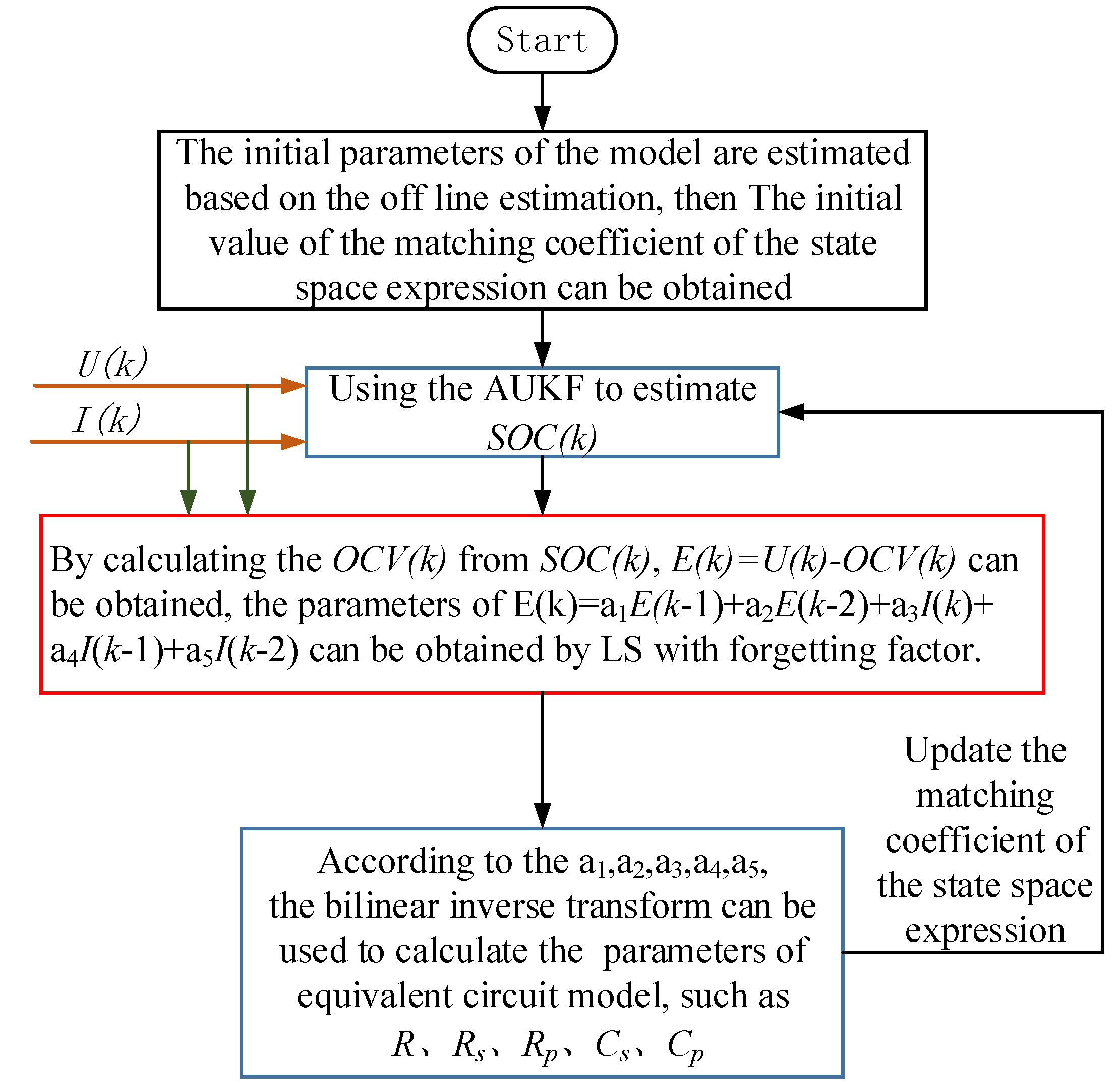
Figure 3 shows the flow chart for identifying the dynamic parameters and verifying the model. According to Figure 3, based on the LS with a forgetting factor, the dynamic parameters of an actual battery is identified and the established model is verified, in combination with the corresponding relation of the battery OCV and the SOC.

Figure 3. Parameter identification flow chart.

Figure 3. Parameter identification flow chart.

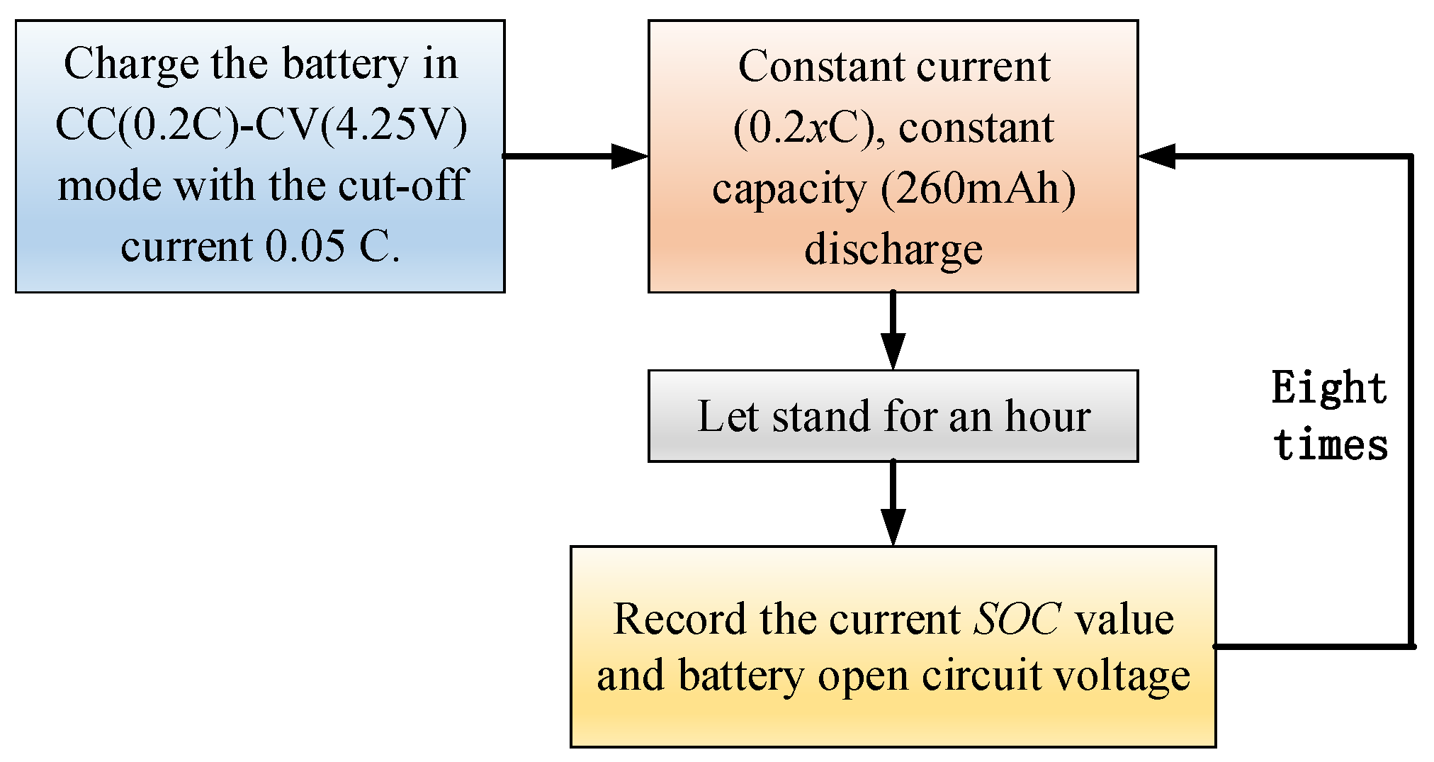
3.1. OCV-SOC Calibration Experiment

In this paper, the discharge experiment, conducted at a constant temperature (25 °C) under intermittent discharge conditions with constant current and capacity, calibrates the OCV-SOC curve with 0.2 C, 0.3 C, 0.4 C, 0.5 C, 0.6 C, 0.75 C, and 1 C. Figure 4 shows the calibration steps of the battery.

Figure 4. Calibration steps of the OCV-SOC.

Figure 4. Calibration steps of the OCV-SOC.

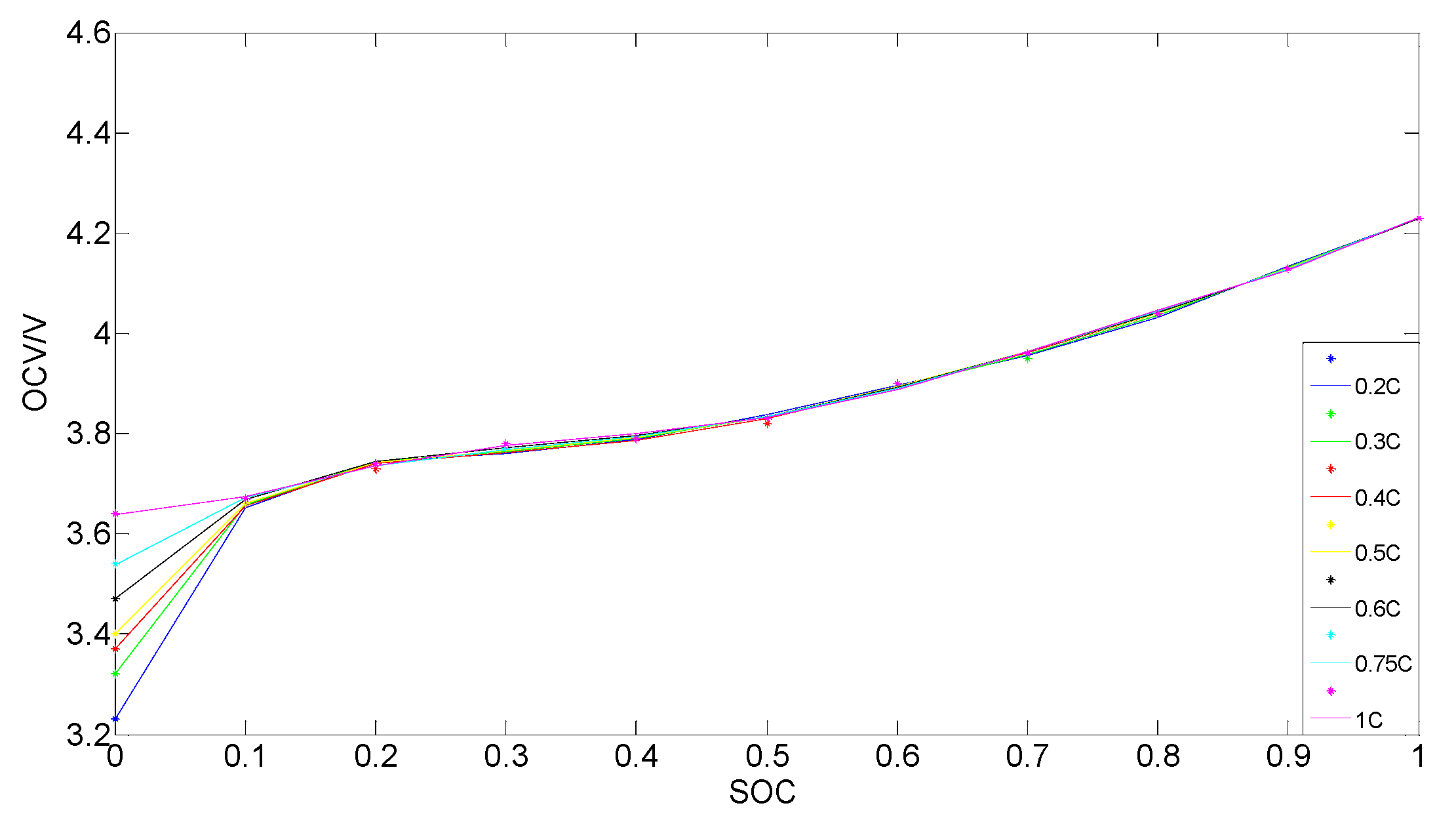
The corresponding relationships between OCV and SOC were recorded for x = 2, 3, 4, 5, 6, 7.5, 10, respectively. Figure 5 shows the different OCV-SOC relationships with sixth order polynomial fittings.

Figure 5. Different OCV-SOC relationships with sixth order polynomial fittings.

Figure 5. Different OCV-SOC relationships with sixth order polynomial fittings.

From Figure 5, when the SOC is above 10%, all the relationships seem to be superposed. This indicates that at the same temperature and the same SOH, any of the curves can be chosen to represent the OCV-SOC relationship. However, a smaller current leads to a smaller change of the battery characteristics. The 0.2 C constant current intermittent discharging OCV-SOC relationship is selected as the reference curve, and the open circuit voltage of the battery as a function of SOC can be represented by Equation (7):

V_oc = b₁ × SOC⁶ + b₂ × SOC⁵ + b₃ × SOC⁴ + b₄ × SOC³ + b₅ × SOC² + b₆ × SOC + b₇

(7)

where a₁ to a₇ are coefficients obtained by the sixth order polynomial fitting giving b₁ = −34.72, b₂ = 120.7, b₃ = −165.9, b₄ = 114.5, b₅ = −40.9, b₆ = 7.31, and b₇ = 3.231.

3.2. Application of LS with a Forgetting Factor

From Formulas (4) and (5), the Laplace equation for the battery model can be deduced:

$$E(s)-U(s)=I(s)(R+\frac{R_s}{1+R_s{C}_{s}s}+\frac{R_p}{1+R_p{C}_{p}s})$$

(8)

Therefore:

$$\begin{array}{ll}G(s)& =(R+\frac{R_s}{1+R_s{C}_{s}s}+\frac{R_p}{1+R_p{C}_{p}s})\\ & =\frac{R{\mathsf{\tau }}_s{\mathsf{\tau }}_p{s}^2+(R{\mathsf{\tau }}_s+R{\mathsf{\tau }}_p+R_p{\mathsf{\tau }}_s+R_s{\mathsf{\tau }}_p)s+R+R_p+R_s}{{\mathsf{\tau }}_s{\mathsf{\tau }}_p{s}^2+({\mathsf{\tau }}_s+{\mathsf{\tau }}_p)s+1}\\ & =\frac{R{s}^2+\frac{1}{{\mathsf{\tau }}_p{\mathsf{\tau }}_s}(R{\mathsf{\tau }}_s+R{\mathsf{\tau }}_p+R_s{\mathsf{\tau }}_p+R_p{\mathsf{\tau }}_s)s+\frac{R+R_s+R_p}{{\mathsf{\tau }}_p{\mathsf{\tau }}_s}}{s^2+\frac{({\mathsf{\tau }}_p+{\mathsf{\tau }}_s)}{{\mathsf{\tau }}_p{\mathsf{\tau }}_s}s+\frac{1}{{\mathsf{\tau }}_p{\mathsf{\tau }}_s}}\end{array}$$

(9)

where ${\mathsf{\tau }}_s$ is the time constant of R_s, C_s, and ${\tau }_p$ is the time constant of R_p, C_p.

Using bilinear transform to discretize Equation (9), $s=\frac{2}{T}\frac{1-z^{-1}}{1+z^{-1}}$ is obtained, and the discrete transfer function is as follows:

$$G(z^{-1})=\frac{a_3+a_4{z}^{-1}+a_5{z}^{-2}}{1-a_1{z}^{-1}-a_2{z}^{-2}}$$

(10)

where a₁, a₂, a₃, a₄, a₅ are the corresponding constant coefficients. Formula (9) can then be converted to a differential equation:

$$y\left(k\right)=E\left(k\right)-U\left(k\right)=a_{1}y\left(k-1\right)+a_{2}y\left(k-2\right)+a_{3}I\left(k\right)+a_{4}I\left(k-1\right)+a_{5}I\left(k-2\right)$$

(11)

where I(k) and y(k) indicate the system input and output, respectively, and subsequently gives:

$$\mathsf{\phi }\left(\mathrm{k}\right)={\left[y\left(k-1\right) y\left(k-2\right) I\left(k\right) I\left(k-1\right) I\left(k-2\right)\right]}^T, \mathsf{\theta }=\left[a_1 a_2 a_3 a_4 a_5\right];$$

If we assume the k moment sensor sampling error is e(k), then:

$$y\left(k\right)={\phi }^T\left(k\right)\mathsf{\theta }+e\left(k\right)$$

(12)

and expanding $\varphi \left(k\right)$ to N-dimensional, where k = 1, 2, 3…N+ n, n = 2, the following equation is deduced:

$$\begin{array}{ll}\{\begin{array}{l}\mathsf{\Phi }(k)=\left[\begin{array}{lllll}y(2)& y(1)& I(3)& I(2)& I(1)\\ y(3)& y(2)& I(4)& I(3)& I(2)\\ ⋮& ⋮& ⋮& ⋮& ⋮\\ y(N+1)& y(N)& I(N+2)& I(N+1)& I(N)\end{array}\right]\\ \\ Y={[y(3)y(4)y(5)\cdots y(N+2)]}^T\\ e={[e(3)e(4)e(5)\cdots e(N+2)]}^T\end{array}& k\ge 3\end{array}$$

(13)

Next, taking the criterion Equation $J\left(\mathsf{\theta }\right)$:

$$J(\mathsf{\theta })={\displaystyle \sum _{i=1}^N{(Y-\mathsf{\Phi }\mathsf{\theta })}^2={\displaystyle \sum _{i=1}^N{(e(i+2))}^2}}$$

(14)

and considering the least squares method is to take the $J\left(\mathsf{\theta }\right)$ minimum:

$$\frac{\partial J(\mathsf{\theta })}{\partial (\mathsf{\theta })}=\frac{\partial }{\partial (\mathsf{\theta })}[{(Y-\mathsf{\Phi }\mathsf{\theta })}^T(Y-\mathsf{\Phi }\mathsf{\theta })]=0$$

(15)

which gives:

$$\widehat{\mathsf{\theta }}={[{\mathsf{\Phi }}^T\mathsf{\Phi }]}^{-1}{\mathsf{\Phi }}^{T}Y$$

(16)

The above equations constitute a one-time least square calculation. However, for the actual system, a one-time calculation does not give an estimated value close to the true value. Thus, a recursive least square method is introduced:

$$\{\begin{array}{c}\widehat{\mathsf{\theta }}\left(k+1\right)=\widehat{\mathsf{\theta }}\left(k\right)+K\left(k+1\right)\left[y\left(k+1\right)-{\mathsf{\Phi }}^T\left(k+1\right)\widehat{\mathsf{\theta }}\left(k\right)\right]\\ K\left(k+1\right)=P\left(k+1\right)\mathsf{\Phi }\left(k+1\right)\\ P\left(k+1\right)=P\left(k\right)-\frac{P\left(k\right)\mathsf{\Phi }\left(k+1\right){\mathsf{\Phi }}^T\left(k+1\right)P\left(k\right)}{I+{\mathsf{\Phi }}^T\left(k+1\right)P\left(k\right)\mathsf{\Phi }\left(k+1\right)}\end{array}$$

(17)

where $\widehat{\mathsf{\theta }}\left(k\right)$ is the system-estimated reference value of the previous cycle, ${\mathsf{\Phi }}^T\left(k+1\right)\widehat{\mathsf{\theta }}\left(k\right)$ is the observed value of this cycle, $y\left(\mathrm{k}+1\right)$ is the actual observed value of the system, ${\mathsf{\Phi }}^T\left(k+1\right)\widehat{\mathsf{\theta }}\left(k\right)$ is the prediction error, and $K\left(\mathrm{k}+1\right)$ is the corrected prediction value. To obtain the optimal estimation of the present cycle, $\mathsf{\theta }\left(0\right)$ and $P\left(0\right)$ must be first provided to meet the requirements, $K\left(\mathrm{k}+1\right)$ is then obtained, and the least square method is executed. Generally, $\widehat{\mathsf{\theta }}\left(0\right)$ can be any value, and $P\left(0\right)=\mathsf{\alpha }I$, where $\mathsf{\alpha }$ is a positive real number, and $I$ is a unit matrix.

The recursive least squares method has an unlimited memory, i.e., as the length K increases, the older data accumulates, making new data difficult to substitute into the least-square steps. This will subsequently affect parameter estimation, especially in time-varying systems. Because a large amount of accumulated old data creates an imbalance with the new data, the newly estimated parameters cannot accurately reflect the characteristics of the system at a current moment. Thus, to avoid the above situation [15], a forgetting factor $\mathsf{\lambda }$, where $0<\mathsf{\lambda }<1$, is introduced:

$$P^{-1}\left(k+1\right)=\mathsf{\lambda }{P}^{-1}\left(k\right)+\mathsf{\Phi }\left(k+1\right){\mathsf{\Phi }}^T\left(k+1\right)$$

(18)

Thus, even when $(N+1$) is large, $P(N+1$) does not go to 0, and “data saturation” can be eliminated.

The steps of the least square algorithm with the forgetting factor are as follows:

$$\{\begin{array}{c}\widehat{\mathsf{\theta }}\left(k+1\right)=\widehat{\mathsf{\theta }}\left(k\right)+K\left(k+1\right)\left[y\left(k+1\right)-{\mathsf{\Phi }}^T\left(k+1\right)\widehat{\mathsf{\theta }}\left(k\right)\right]\\ K\left(k+1\right)=P\left(k\right)\mathsf{\Phi }\left(k+1\right){\left[\lambda +{\mathsf{\Phi }}^T\left(k+1\right)P\left(k\right)\mathsf{\Phi }\left(k+1\right)\right]}^{-1}\\ P\left(k+1\right)=\frac{1}{\lambda }\left[I-K\left(k+1\right){\mathsf{\Phi }}^T\left(k+1\right)\right]P\left(k\right)\end{array}$$

(19)

In Equation (19), $\mathsf{\lambda }=1$ the most common least squares. When $\mathsf{\lambda }$ is smaller, the tracking ability is stronger, but the volatility is greater; hence, generally 0.95 < $\mathsf{\lambda }$ < 1.

3.3. Dynamic Parameter Identification

Parameter identification is based on the information of the measurement system and provides guidelines to estimate the model structure and unknown parameters. According to the value of $\mathsf{\theta }$ derived from the previous algorithm:

$$z^{-1}=\frac{1-\frac{T}{2}s}{1+\frac{T}{2}s}$$

(20)

Substituting this into Equation (10):

$$G(s)=\frac{\frac{a_3-a_4+a_5}{1+a_1-a_2}{s}^2+\frac{4(a_3-a_5)}{T(1+a_1-a_2)}s+\frac{4(a_3-a_4+a_5)}{T^2(1+a_1-a_2)}}{s^2+\frac{4(1+a_2)}{T(1+a_1-a_2)}s+\frac{4(1-a_1-a_2)}{T^2(1+a_1-a_2)}}$$

(21)

Because the corresponding coefficients of Equations (9) and (21) are equal, we can obtain:

$$\{\begin{array}{c}R=\frac{a_3-a_4+a_5}{1+a_1-a_2}\\ {\tau }_s{\tau }_p=\frac{T^2(1+a_1-a_2)}{4(1-a_1-a_2)}\\ {\tau }_s+{\tau }_p=\frac{T(1+a_2)}{1-a_1-a_2}\\ R+R_s+R_p=\frac{a_3-a_4+a_5}{1-a_1-a_2}\\ R{\tau }_s+R{\tau }_p+R_p{\tau }_s+R_s{\tau }_p=\frac{4(a_3-a_5)}{T(1+a_1-a_2)}\end{array}$$

(22)

The coefficients on the right-hand side of Equation (22) can be obtained by a recursive algorithm, and the variables on the left-hand side are the unknown parameters of the battery model. This completes the process of parameter identification.

In the process of identifying model parameters, the known variables are V(k), I(k), V(k−1), I(k−1), SOC(k−1) and V(k−2), I(k−2), and the unknown variable is $\mathsf{\theta }={\left[a_1 a_2 a_3 a_4 a_5\right]}^T$. The steps of using the LS method with a forgetting factor for the identification of dynamic parameters of the battery are as follows:

• Identification initialization using sampling time T = 1s, and SOC (0) = 90%.
• Calculate $V_{oc}\left(k\right)-V\left(k\right)$ each time and obtain the input $\mathsf{\Phi }\left(k\right)$ and output $y\left(\mathrm{k}\right)$ of the identification process accurately.
• Initialize $\mathsf{\theta }\left(0\right)$, $P\left(0\right)$ and the forgetting factor $\mathsf{\lambda }$, and start the forgetting factor least square parameter identification; in this paper, $\mathsf{\alpha }=5000,\mathsf{\lambda }=0.96$.

Using this process, the value of $\theta$ can be obtained, and then according to Equation (22), R, R_s, R_p, C_s, and C_p can consequently be obtained; hence, the dynamic real-time update of the battery model parameters is realized, along with an accurate description of the dynamic response of the battery. Furthermore, the accuracy of the battery model is improved, and the basis for estimating the battery SOC accurately is provided in latter sections.

3.4. Model Verification

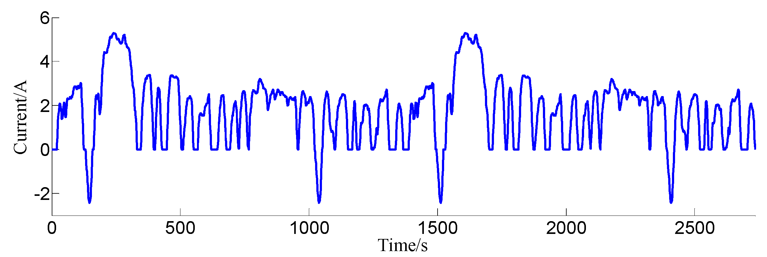
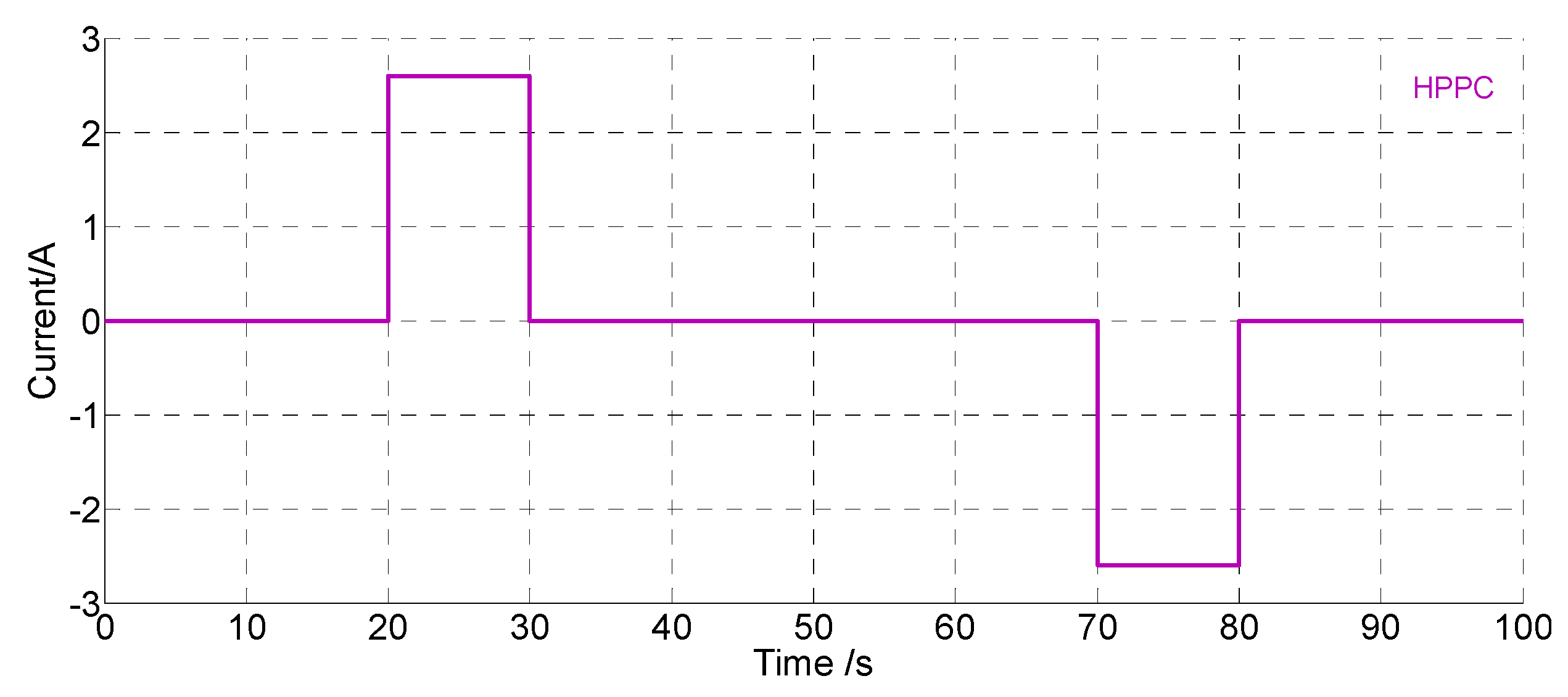
After the dynamic parameters of the battery model are determined, the next step is to verify the accuracy of the model using Hybrid Pulse Power Characterization (HPPC) [16]. Here, the initial SOC is set to 0.5, and the input current waveform is shown in Figure 6 with a pulse current size of 1 C (2.6 A).

Figure 6. HPPC pulse current.

Figure 6. HPPC pulse current.

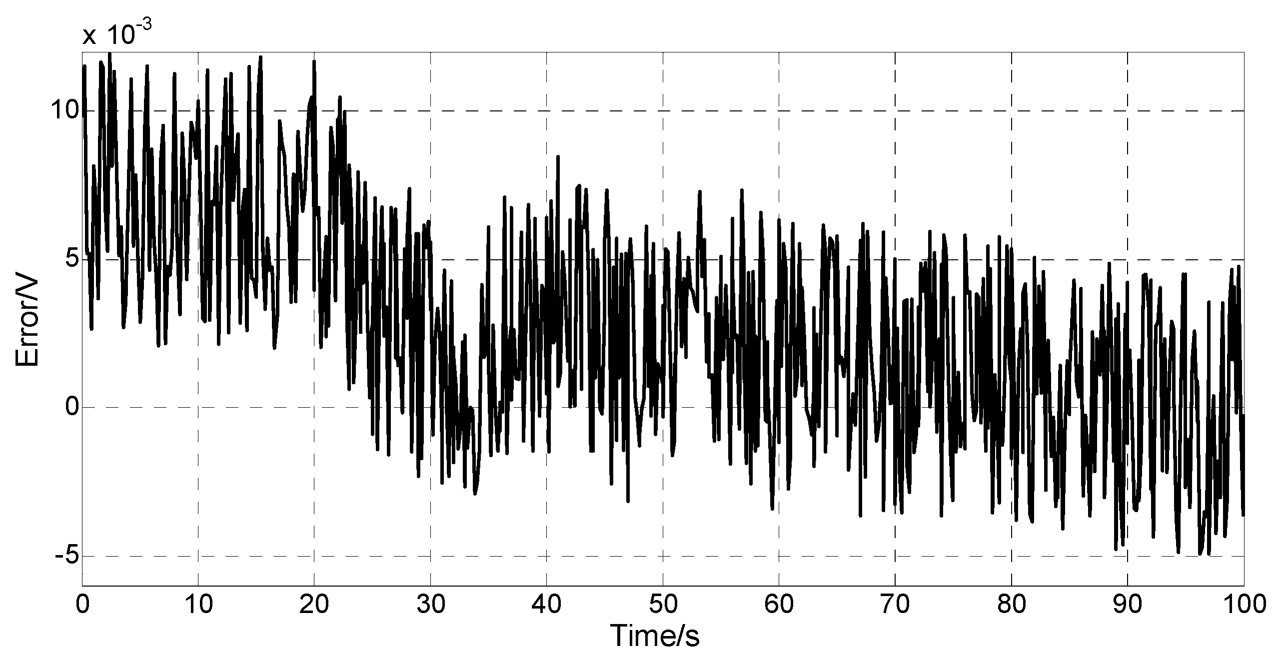
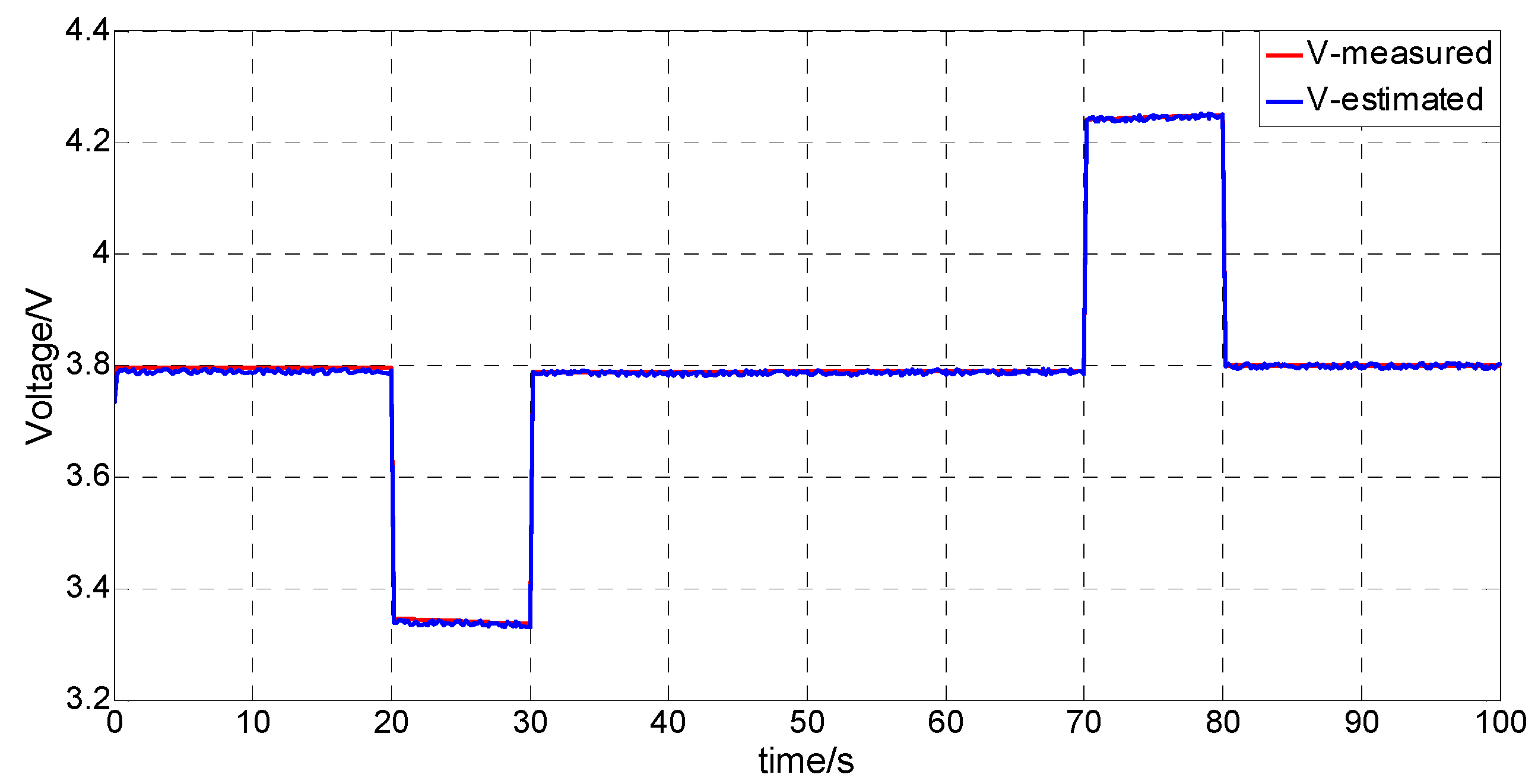
A comparison of voltage responses is shown in Figure 7, and Figure 8 depicts the voltage error, i.e., the differences between the measured and estimated voltages.

Figure 7. Comparison of voltage responses.

Figure 7. Comparison of voltage responses.

Figure 8. Differences between measured and estimated voltages.

Figure 8. Differences between measured and estimated voltages.

Figure 7 and Figure 8 show that when the current suddenly changes, the model estimated voltage can track the actual voltage well, and the error remains at approximately 0.01 V. Hence, this model can be used to verify the algorithms of the SOC estimation in this paper.

4. Establishment of the AUKF Algorithm

The main idea of the Kalman filter is to make an optimal estimation of the minimum mean square value, which includes the following two stages: prediction and updating. In the prediction stage, the filter makes an estimate of the current state according to the value of the last state. In the updating stage, according to the observed value of the current state, the filter optimizes the predicted value from the prediction stage to obtain a more accurate estimation of the current state.

It is important to note that the Kalman filter is mainly used in linear systems, while a battery system reflects complex nonlinear characteristics. Some people [4,7,8] have used the extended Kalman filter (EKF) for SOC estimation, and while some good results have been achieved, linearization errors are inevitable, and the Jacobian matrix is also difficult to estimate. In recent years, a new nonlinear filtering method has emerged, collectively referred to as the sigma point Kalman filter, including the unscented Kalman filter (UKF). UKF does not require Taylor approximations of nonlinear equations; instead, the nonlinear unscented transform (UT) technique is used directly, and thus the mean and the variance of the nonlinear system states can be mapped directly to achieve a higher estimation accuracy.

In a normal UKF algorithm [17,18], the covariance is a constant and cannot satisfy the real-time dynamic characteristics of the noise, which has a certain impact on the accuracy. In this paper, to eliminate this effect, the normal UKF algorithm is improved by updating the covariance in real-time and thus improving the accuracy of the UKF. This type of algorithm is called the adaptive unscented Kalman filter (AUKF) algorithm. The establishment process of the algorithm is described as follows.

A discrete-time controlled system is governed by the equation of state and the observation equations are shown in Equation (23):

$$\{\begin{array}{c}{x}_{k+1}=A_x{x}_k+B_k{u}_k+w_k\\ y_k=C_k{x}_k+D_k{u}_k+v_k\end{array}$$

(23)

where the random variables w_k and v_k represent the process and measurement noise, respectively. As for the UKF, the iteration equation is based on a certain set of sample points, which is chosen to make their mean value and variance consistent with the mean value and variance of the state variables. Then, these points will recycle the equation of the discrete-time process model to produce a set of predicted points. After that, the mean value and the variance of the predicted points will be calculated to modify the results, and the mean value and the variance will be estimated. Before the UKF recursion, the state variables must be modified in a superposition of the process noise and the measurement noise of the original states. The SOC of the Li-ion battery pack can be calculated using the ampere-hour integral method:

$$SOC\left(t\right)=\text{SOC}\left(t^{\prime }\right)-\frac{1}{C_N}{{\displaystyle \int }}_{t^{\prime }}^t\mathsf{\eta }idt$$

(24)

In Equation (24), $\mathsf{\eta }=\frac{k_t{k}_i}{k_c}$, where k_i is the compensation coefficient of charge and discharge rate, k_t is the temperature compensation coefficient, and k_c is the compensation coefficient of cycles. C_N is the actual available battery capacity.

The Li-ion battery equation of state can be obtained from Equations (4) and (24):

$$\left[\begin{array}{c}SO{C}_k\\ u_{s,k}\\ u_{p,k}\end{array}\right]=\left[\begin{array}{ccc}1& 0& 0\\ 0& a_s& 0\\ 0& 0& a_p\end{array}\right]\left[\begin{array}{c}SO{C}_{k-1}\\ u_{s,k-1}\\ u_{p,k-1}\end{array}\right]+\left[\begin{array}{c}-\mathsf{\eta }T/C_N\\ b_s\\ b_p\end{array}\right]I_{k-1}+\left[\begin{array}{c}{w}_1\left(k\right)\\ w_3\left(k\right)\\ w_5\left(k\right)\end{array}\right]$$

(25)

$$U_k=E_k-I_{k}R-U_{s,k}-U_{p,k}+v\left(k\right)=F\left(SO{C}_k\right)-I_{k}R-U_{s,k}-U_{p,k}+v\left(k\right)$$

(26)

For the circuit model shown in the Equations (25) and (26):

$$X_k={\left[x_k^T, w_k^T, v_k^T\right]}^T={\left[SO{C}_k, u_{s,k}, u_{p,k}, w_{soc,k}, w_{s,k}, w_{p,k}, v_k\right]}^T$$

(27)

To facilitate the distinction, we can take $x_k=\left[SO{C}_k, U_{s,k}, U_{p,k}\right]$ as the initial state of the system, y_k as the raw output (its corresponding symbol is U_k in the circuit model of the Li-ion battery), u_k as the control variable (its corresponding symbol is I_k), and make $\mathsf{\Psi }=\left[y_1,y_2,y_3,\cdots ,y_k \right]$. The operations of an ordinary UKF are as follows.

First, select (2L + 1) sampling points, and make Sample=$\left\{z_i,X_{k-1,i}\right\}$, $i$=0, 1, 2, $\cdots ,2L+1$, where $X_{k-1,i}$ is the selected points and $z_i$ is the corresponding weighting value. Then, select the points in the following manner:

$$\{\begin{array}{c}{X}_{k-1,0}={\widehat{X}}_{k-1} \\ X_{k-1,i}={\widehat{X}}_{k-1}+{\left(\sqrt{\left(L+\lambda \right)P_{X,k-1}}\right)}_i i=1~L\\ X_{k-1,i}={\widehat{X}}_{k-1}-{\left(\sqrt{\left(L+\lambda \right)P_{X,k-1}}\right)}_i i=\left(L+1\right)~2L \end{array}$$

(28)

The corresponding weighting values are:

$$\{\begin{array}{c}{z}_0^{\left(m\right)}=\frac{\lambda }{L+\lambda }\\ z_0^{\left(c\right)}=\frac{\lambda }{L+\lambda }+\left(1+{\mathsf{\alpha }}^2+\beta \right)\\ z_i^{\left(m\right)}=z_i^{\left(c\right)}=\frac{1}{2\left(L+\lambda \right)} i=1~2L\end{array}$$

(29)

where $\mathsf{\lambda }={\mathsf{\alpha }}^2\left(L+t\right)-L$, $z^{\left(m\right)}$ is the corresponding weighting value of the mean, $z^{\left(c\right)}$ is the corresponding weighting value of the variance, and ${\left(\sqrt{\left(L+\lambda \right)P_{X,k-1}}\right)}_i$ denotes the column i of the square-rooting matrix $\left(L+\lambda \right)P_{X,k-1}$. To ensure that the covariance matrix is definitely positive, we must take $\mathrm{t}\ge 0$; $\mathsf{\alpha }$ controls the distance of the selected points, with ${10}^{-2}\le \alpha \le 1$, and $\mathsf{\beta }$ is used to reduce the error of the higher-order terms. For a Gaussian, the optimal choice is $\mathsf{\beta }=2$ in this paper, along with $t=0$ and $\alpha =1$. ${\widehat{X}}_{k-1,i}$ consists of ${\widehat{X}}_{k-1,i}^x, {\widehat{X}}_{k-1,i}^w$ and ${\widehat{X}}_{k-1,i}^v$.

The time updates of the iterative process are as follows:

$$\{\begin{array}{c}{\widehat{X}}_{k|k-1}=E\{[f(x_{k-1},u_{k-1})+{\omega }_{k-1}]|{\mathsf{\Psi }}_{k-1}\}={\displaystyle {\displaystyle \sum }_{i=0}^{2L}}{z}_i^{\left(m\right)}[A_{k-1}{x}_{k-1,i}^x+B_{k-1}{u}_{k-1}+x_{k-1,i}^w]={\displaystyle {\displaystyle \sum }_{i=0}^{2L}}{z}_i^{\left(m\right)}{X}_{k|k-1,i}^x\\ P_{x,k|k-1}=E[{(x_k-{\widehat{x}}_{k|k-1})(x_k-{\widehat{x}}_{k|k-1})}^T]={\displaystyle {\displaystyle \sum }_{i=0}^{2L}}{z}_i^{\left(c\right)}(X_{k|k-1,i}^x-{\widehat{x}}_{k|k-1}){(X_{k|k-1,i}^x-{\widehat{x}}_{k|k-1})}^T\\ {\widehat{y}}_k=E\{[h(x_k,u_k)+{\nu }_k]|{\mathsf{\Psi }}_{k-1}\}={\displaystyle {\displaystyle \sum }_{i=0}^{2L}}{z}_i^{\left(m\right)}[h(X_{k|k-1,i}^x,u_k)+x_{k-1,i}^{\nu }]={\displaystyle {\displaystyle \sum }_{i=0}^{2L}}{z}_i^{\left(m\right)}{y}_{k|k-1,i}\end{array}$$

(30)

The gain matrix of the filter is:

$$L_k=P_{xy,k}{P}_{y,k}^{-1}={\displaystyle \sum }_{i=0}^{2L}{z}_i^{\left(c\right)}\left(X_{k|k-1,i}^x-{\widehat{x}}_{k|k-1}\right){\left(y_{k|k-1,i}-{\widehat{y}}_k\right)}^T{[{\displaystyle \sum }_{i=0}^{2L}{z}_i^{\left(c\right)}\left(y_{k|k-1,i}-{\widehat{y}}_k\right){\left(y_{k|k-1,i}-{\widehat{y}}_k\right)}^T]}^{-1}$$

(31)

The estimates of the states and the mean square error are as follows:

$$\{\begin{array}{c}{x}_k={\widehat{x}}_{k|k-1}+L_k\left(y_k-{\widehat{y}}_k\right)\\ P_{x,k}=P_{x,k|k-1}-L_k{P}_{y,k}{L}_k^T\end{array}$$

(32)

where y_k is the actual measured value of the system output. As the process noise and measurement noise are real-time and to make the covariance of the process noise and measurement noise update in real time, the following is needed:

$$\{\begin{array}{c}{\mu }_k=y_k-H\left[{\widehat{x}}_k,u_k\right]\\ F_k={\mu }_k{\mu }_k^T\\ R_k^v=(F_k+{\displaystyle {\displaystyle \sum }_{i=0}^{2L}}{z}_i^c(y_{k|k-1,i}-y_k){\left(y_{k|k-1,i}-y_k\right)}^T)/2\\ R_k^w=L_k{F}_k{L}_k^T\end{array}$$

(33)

where ${\mathsf{\mu }}_k$ is the residual error of the system measured output and $y_{k|k-1,i}$ is the residual error of the system measured output estimated by the sigma points.

5. Experiments with the SOC Estimation Algorithm

5.1. Reasons and Steps of the Joint Estimation Algorithm

The LS method with a forgetting factor undertakes the work of parameter identification, and the AUKF functions in the progress of the SOC estimation. The characteristics of these two algorithms [17,18,19,20] are shown in Table 1.

Table 1. The characteristics of the two algorithms.

Algorithm	Advantages	Disadvantages
LS with a forgetting factor	This algorithm does not require the observation data to provide the probability and statistics of the noise under random conditions; the statistical properties are quite good.	This algorithm cannot identify an unbiased, coherent parameter with colored noise.
AUKF	This algorithm has a strong immunity to the disturbance of the initial value; the iterative calculations ensure the acquirement of the desired value.	In theory, the minimum variance estimation can be obtained only when the statistical properties are known.

Table 1. The characteristics of the two algorithms.

Algorithm	Advantages	Disadvantages
LS with a forgetting factor	This algorithm does not require the observation data to provide the probability and statistics of the noise under random conditions; the statistical properties are quite good.	This algorithm cannot identify an unbiased, coherent parameter with colored noise.
AUKF	This algorithm has a strong immunity to the disturbance of the initial value; the iterative calculations ensure the acquirement of the desired value.	In theory, the minimum variance estimation can be obtained only when the statistical properties are known.

Based on the merits and the drawbacks mentioned above, a joint algorithm of these two algorithms is proposed. The implementation of the joint algorithm can be divided briefly into two steps. First, the Kalman filter model updates parameters using the data provided by the LS method with a forgetting factor. Then, the filter generates the SOC, which will be used to deduce the OCV. Second, the OCV combines the measured voltage and the current value to update the LS estimation result for the next reiteration. Figure 9 illustrates the steps of the joint algorithm.

Figure 9. The combination of the LS method with a forgetting factor and the AUKF.

Figure 9. The combination of the LS method with a forgetting factor and the AUKF.

The details of the implemented algorithm are as follows:

• The BMS measures the voltage of the Li-ion battery in the static state, according to the function of OCV-SOC, and the initial value of SOC (0) is calculated.
• The initial values of the model, i.e., R(0), R_s(0), R_p(0), C_s(0), and C_p(0), are estimated, according to the current and voltage responses in the early stage of battery operation.
• The initial values of the model are used to calculate the initial coefficients, and then the adaptive unscented Kalman Filter will be used to obtain the SOC value at the current moment.
• The open circuit voltage V_oc at that time is calculated according to the function relationship of OCV-SOC. Then, the parameters of the model at the current instance are obtained using the LS method with a forgetting factor.
• The model parameters are utilized to update the corresponding coefficients, and the AUKF is used again to calculate the estimated value of SOC in the next instance, and step 4 is repeated.

Step 4 is applied to calculate the model parameters, and step 5 is utilized to estimate the SOC values. These two steps are repeated, and the Li-ion battery parameters and the estimated SOC values at every instance will be obtained.

5.2. Experimental Analysis of the Joint Estimation Algorithm

In this section, simulations of the joint algorithm mentioned above and a single AUKF are presented, and analysis will be made on the accuracy of the algorithms and the convergence to the initial value error.

In the process of setting the battery discharging and charging states, to correspond to the experimental object in the OCV-SOC calibration, the current signal in Figure 10 is adopted to describe the increase or decrease of the current in the discharging or charging process of the power battery. In one period, the average output current is 1.77 A, and the maximum discharging current is 5.28 A, the maximum charging current is 2.42 A. Each period is 1367 s, and the condition lasts two periods.

Figure 10. The input current waveform.

Figure 10. The input current waveform.

5.2.1. Accuracy Verification

In this simulation model, the input current I(k) is integrated using the Ampere-hour (Ah) integral method. As there is no error in the current measurement due to outside disturbances, no accumulative error exists; thus, the integration of the current in the simulation model could be regarded as the theoretical value of the SOC. Figure 11 displays a comparison of the results generated by the two algorithms and the theoretical value. Figure 12 compares the error of these two algorithms.

Figure 11 and Figure 12 illustrate that both algorithms are able to follow the theoretical values of SOC. The maximum error of the joint estimation algorithm is 1.3% and that of AUKF is 2.5%, which indicates a greater accuracy of the joint estimation algorithm.

Figure 11. Comparison of the SOC estimates.

Figure 11. Comparison of the SOC estimates.

Figure 12. Comparison of the SOC estimation error.

Figure 12. Comparison of the SOC estimation error.

5.2.2. Convergence to the SOC Initial Value Error

In the early operational stage of the Li-ion battery, errors exist between the measured and real voltage and current values, which will subsequently lead to an erroneous SOC value. Taking this condition into consideration, the convergence to the initial value error is a vital performance index of an algorithm. This section will discuss this issue. We assume that the real initial value of the SOC is 1, while a SOC value of 0.96 is deduced from the measurements. Figure 13 shows the theoretical value and results of the two algorithms, and Figure 14 is the error comparison of these two algorithms in a time period of 100 s.

Figure 13 and Figure 14 indicate that both algorithms have the ability to converge to the SOC initial value error. At 100 s, the error percentage of the joint estimation algorithm is 1.628%, while that of the AUKF is higher at 3.054%; hence, the joint estimation algorithm is better at converging to the SOC initial value error.

Figure 13. Results of the theoretical value and the two algorithms.

Figure 13. Results of the theoretical value and the two algorithms.

Figure 14. Error comparison in a time period of 100 s.

Figure 14. Error comparison in a time period of 100 s.

6. Conclusions

Power battery SOC is a vital state information of an electrical vehicle and is strongly nonlinear and time-varying. The proposed joint estimation algorithm combines the LS method with a forgetting factor and the AUKF method. This work can be summarized as follows:

• A battery model was built according to its external characteristics, and the parameters were identified and verified at the same time.
• The advantages and disadvantages of the LS method with a forgetting factor and the AUKF method were analyzed, and a joint estimation algorithm was proposed.
• Comparison of the joint estimation algorithm and the AUKF, including the accuracy and the ability to converge to initial value errors, were conducted, and it was concluded that the joint estimation was better than the AUKF.

Suggested future research directions building off of the current data are as follows:

• All of the current data are obtained in a constant temperature environment. Thus, data of the battery operating in a variable temperature environment should be obtained in the future, to evaluate the exact relationship of SOC-OCV.
• The calculations in this paper do not consider the battery health; hence, the joint estimation algorithm should be applied on batteries with different battery health conditions.