One-Dimensional Modeling of an Entrained Coal Gasification Process Using Kinetic Parameters

Abstract

A one-dimensional reactor model was developed to simulate the performance of an entrained flow gasifier under various operating conditions. The model combined the plug flow reactor (PFR) model with the well-stirred reactor (WSR) model. Reaction kinetics was considered together with gas diffusion for the solid-phase reactions in the PFR model, while equilibrium was considered for the gas-phase reactions in the WSR model. The differential and algebraic equations of mass balance and energy balance were solved by a robust ODE solver, i.e., an semi-implicit Runge–Kutta method, and by a nonlinear algebraic solver, respectively. The computed gasifier performance was validated against experimental data from the literature. The difference in product gas concentration from the equilibrium model, and the underlying mechanisms were discussed further. The optimal condition was found after parameter studies were made for various operating conditions.

1. Introduction

There is growing interest in entrained flow gasifiers to produce synthesis gas and generate electric power. They achieve high rates of gasification, producing a relatively clean gas, because they operate at high temperatures with small coal particles. Meanwhile, low rank coal (LRC) is getting more attention because of its advantages over high rank coal, evaluated in terms of long-term availability and cheaper market prices. However, inadvertent use of unconventional fuels such as LRC in an existing gasifier may increase the unconverted carbon, thus reducing the amount of synthesis gas produced [1,2]. In particular, this effect is even more significant because of the high moisture and volatile content in LRC, leading to heavy tar and char formation [3]. This issue is of much concern in an air-blown gasifier operated at lower temperatures. A two-stage scheme has been used to ensure complete carbon conversion in that type of gasifier [4]. A heat-recovery and gas treatment system are also required downstream of an entrained flow gasifier. Sulfuric acid and particulates are typically removed by a wet scrubbing system. The presence of unconverted carbon and tarry material in the synthesis gas causes difficulties in the heat exchange system. Therefore, it is essential to estimate the amount and size of unconverted carbon in the product gas.

In fact, a two-phase approach to account for unconverted carbon in the solid phase has been implemented by using an equilibrium model [5,6,7]. In these works, the variation of product gas composition with oxygen and steam/fuel ratio was evaluated and described in more detail. The dominant factors were found to be temperature, oxygen addition, and gaseous reactions such as the water–gas shift (WGS) reaction. The importance of carbon conversion was identified as governing the gasification process at relatively low oxygen/fuel ratios. However, relative contribution of this mechanism in the equilibrium model may not be similar to one predicted from the one-dimensional kinetic model. For example, the role of the carbon conversion reaction involving solid phasemay be more important in affecting the gas composition than other factors. To the best of our knowledge, no comparison was made between the kinetic reactor model data and the equilibrium model data for carbon conversion and the resultant gas composition. Besides, such differences in the process-determining mechanism have not been discussed in previous works.

In the past, simulation studies were conducted in which the unconverted carbon was predicted by introducing different levels of reaction kinetics and mixing. Ubhayakar et al., used a one-dimensional flow model that considered axial mixing. However, they neglected the solid phase reactions and considered only the gas-phase reactions of volatile products [8]. Wen and Chaung adopted a cell-in-series approach to describe the mixing in a Texaco pilot plant entrained flow gasifier [9]. Each cell was treated as a perfect well-stirred reactor (WSR) for the gas phase, while the solid phase was assumed to be in the plug flow reactor (PFR) condition. Govind and Shah refined the above model by using momentum balance instead of the Stokes’ law approximation for particle velocity calculation [10]. In both investigations, parametric studies were conducted to provide a better understanding of the sensitivity of reactor performance to various operating conditions. A wider range of oxygen/coal and steam/coal ratios was examined. Wu et al., used a zonal approach and the PFR model requiring kinetic parameters for all gas-phase and solid-phase reactions [11]. However, their model validity was assessed by a comparison of the computed results with previous experimental data at a single oxygen/coal ratio.

Vamvuka et al., predicted gasifier performance at various operating conditions [12,13]. They used the PFR model for both the gas and the solid phases. However, they considered finite reaction rates for solid-phase reactions, while assuming equilibrium (i.e., infinite reaction rates) for gas-phase reactions. Their work was mainly concerned with the gasification of coal samples of 40 μm, which is 10 times smaller than the 400 μm coal used in Wen’s work [9]. The former is much closer to the ranges actually used in current industrial gasifiers. The response of product gas composition to oxygen/fuel and steam/fuel ratios appears to be consistent with the results of both Wen and Govind, when the comparison is done with corresponding ranges. However, the coal conversion decreased as the steam/coal ratio increased, irrespective of the oxygen/coal ratio (which was set to 0.5–0.8). This trend is different from that of both Wen and Govind. The optimal range of the steam/coal ratio, where the carbon conversion was maximized, occurred at 0.3–0.6. Therefore, there was a discrepancy with the carbon conversion data at different operating conditions. Furthermore, there was a lack of experimental data with which to validate carbon conversion data owing to associated difficulties such as high pressure condition. There are other previous studies using two parallel ideal reactors to describe a fluidized bed reactor. One reactor is a WSR to simulate the gas flow pattern inside the emulsion phase. The other is a PFR to explain the gas behaviour inside the bubble phase [14,15].

In this study, a one-dimensional reactor model was developed to simulate the performance of an entrained flow gasifier, which focused particularly on carbon conversion. This model combined the PFR model with the WSR model. Reaction kinetics and gas diffusion were considered for the solid-phase reactions in the PFR model, while equilibrium was considered for the gas-phase reactions in the WSR model. A time-efficient semi-implicit Runge–Kutta method with a proprietary variable step size technique was used to solve the differential equations of mass and energy balance of the solid-phase particles. A nonlinear algebraic equation solver was used to solve the system of algebraic equations for the gas-phase components. The predicted gasifier behaviors were compared with experimental data as well as with equilibrium data under various operating conditions. The difference from the equilibrium data and the underlying mechanisms were discussed further.

2. Numerical Model and Solution Section

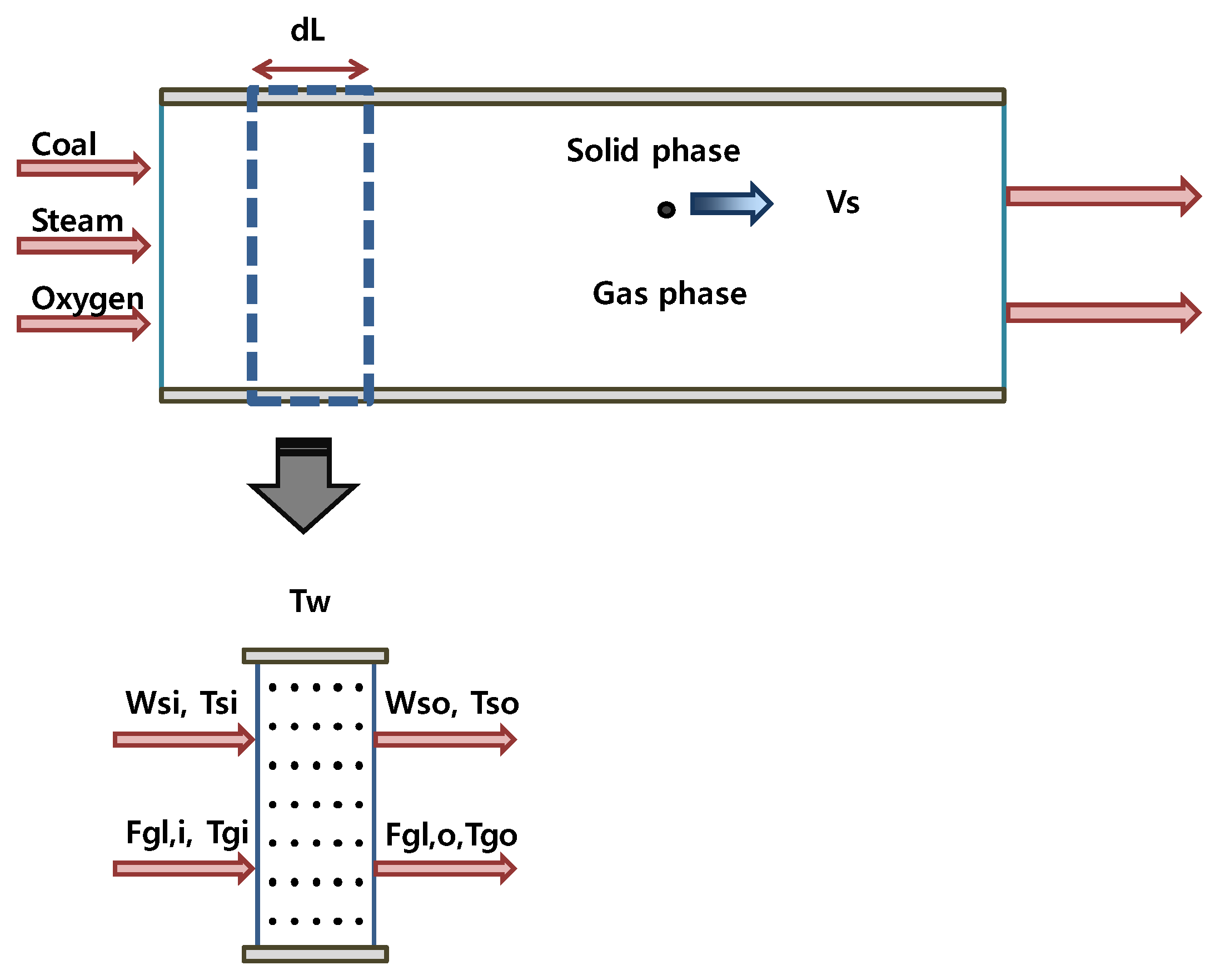
2.1. Model Description and Assumptions

The entrained flow gasifier used in this study is a downflow reactor with concurrent flow of solid and gaseous streams. Pulverized coal and hot gas stream of steam and oxygen are mixed at the reactor entrance and travel concurrently through the reactor. The dispersion of coal in gas is considered to move in plug flow axially through the reactor [16,17]. In the present model, we followed a partitioning zonal approach. The coal particles are pyrolyzed, burned, and gasified along the gasifier. The gasifier was divided into two different reaction zones: the coal combustion zone and the subsequent gasification zone. The pyrolysis and volatile combustion zone was neglected. Wen and Chaung [9] used the one-step model with the rate expression proposed by Badzioch and Hawksley [18] for pyrolysis, and assumed complete conversion for volatile combustion. The pressure effect was further accounted for by the final amount of volatile gas products. However, the partitioning of total yield into detailed composition was difficult because it depends significantly on fuel properties, operating conditions, and solid residence time. Therefore, use of that treatment is limited to certain types of coal. Accordingly, their contribution to the gas composition was excluded in this calculation. Some amounts of heat and gas that are released during this process were alternatively simulated by char reactions and concurrent gas-phase reactions in the coal combustion and gasification zones.

In the first reaction zone, the coal reacts with the oxygen to produce CO, CO₂, and H₂O, and with steam and CO₂ to produce CO and H₂. The combustible gases, CO and H₂, in turn react in the gas phase with oxygen to produce more heat. Because of rapid combustion, most of the oxygen is consumed. The key reactions chosen to represent the essential features of the gasification process are listed in Table 1. There are three gas-phase reactions and four solid-phase reactions. The conditions in the combustion zone are such that both the temperatures and the concentrations of carbon dioxide and steam are high. Therefore, the gas-phase combustions are found to be instantaneous enough to be described by the equilibrium model.

Table 1. Solid- and gas-phase reactions in each reaction zone.

Reaction Zones			Solid Phase (k)	Gas Phase (j)
Coal combustion/gasification			1,2,3,4	1,2,3
Coal gasification/reduction			1,2,3,4	3,4
k	Solid Phase Reaction
1	$C_a{H}_b{O}_c{N}_d{S}_e+(\frac{a}{\mathsf{\varphi }}+\frac{b}{4}-\frac{c}{2}-\frac{e}{2})O_2\to (\frac{2}{\mathsf{\varphi }}-1)aC{O}_2+2(1-\frac{1}{\mathsf{\varphi }})aCO+(\frac{b}{2}-e)H_{2}O+e{H}_{2}S+\frac{d}{2}{N}_2$*
2	$C_a{H}_b{O}_c{N}_d{S}_e+aC{O}_2\to 2aCO+c{H}_{2}O+(\frac{b}{2}-c-e)H_2+e{H}_{2}S+\frac{d}{2}{N}_2$
3	$C_a{H}_b{O}_c{N}_d{S}_e+(a-c)H_{2}O\to aCO+(a+\frac{b}{2}-c-e)H_2+e{H}_{2}S+\frac{d}{2}{N}_2$
4	$C_a{H}_b{O}_c{N}_d{S}_e+(2a-\frac{b}{2}+c+e)H_2\to aC{H}_4+c{H}_{2}O+e{H}_{2}S+\frac{d}{2}{N}_2$
j	Gas Phase Reaction			Remarks
1	$CO+\frac{1}{2}{O}_2\rightleftharpoons C{O}_2$			CO oxidation
2	$H_2+\frac{1}{2}{O}_2\rightleftharpoons H_{2}O$			H2 oxidation
3	$CO+H_{2}O\rightleftharpoons C{O}_2+H_2$			WGS
4	$CO+3H_2\rightleftharpoons C{H}_4+H_{2}O$			Methane-steam

*$\mathsf{\varphi }=\frac{2z+2}{z+2}\begin{array}{c}where\end{array}\begin{array}{c}z=2500\cdot \exp (-\frac{6249}{T}\end{array})$ from the reference [13].

Table 1. Solid- and gas-phase reactions in each reaction zone.

Reaction Zones			Solid Phase (k)	Gas Phase (j)
Coal combustion/gasification			1,2,3,4	1,2,3
Coal gasification/reduction			1,2,3,4	3,4
k	Solid Phase Reaction
1	$C_a{H}_b{O}_c{N}_d{S}_e+(\frac{a}{\mathsf{\varphi }}+\frac{b}{4}-\frac{c}{2}-\frac{e}{2})O_2\to (\frac{2}{\mathsf{\varphi }}-1)aC{O}_2+2(1-\frac{1}{\mathsf{\varphi }})aCO+(\frac{b}{2}-e)H_{2}O+e{H}_{2}S+\frac{d}{2}{N}_2$*
2	$C_a{H}_b{O}_c{N}_d{S}_e+aC{O}_2\to 2aCO+c{H}_{2}O+(\frac{b}{2}-c-e)H_2+e{H}_{2}S+\frac{d}{2}{N}_2$
3	$C_a{H}_b{O}_c{N}_d{S}_e+(a-c)H_{2}O\to aCO+(a+\frac{b}{2}-c-e)H_2+e{H}_{2}S+\frac{d}{2}{N}_2$
4	$C_a{H}_b{O}_c{N}_d{S}_e+(2a-\frac{b}{2}+c+e)H_2\to aC{H}_4+c{H}_{2}O+e{H}_{2}S+\frac{d}{2}{N}_2$
j	Gas Phase Reaction			Remarks
1	$CO+\frac{1}{2}{O}_2\rightleftharpoons C{O}_2$			CO oxidation
2	$H_2+\frac{1}{2}{O}_2\rightleftharpoons H_{2}O$			H2 oxidation
3	$CO+H_{2}O\rightleftharpoons C{O}_2+H_2$			WGS
4	$CO+3H_2\rightleftharpoons C{H}_4+H_{2}O$			Methane-steam

*$\mathsf{\varphi }=\frac{2z+2}{z+2}\begin{array}{c}where\end{array}\begin{array}{c}z=2500\cdot \exp (-\frac{6249}{T}\end{array})$ from the reference [13].

The combusted gas flows into the gasification zone, which is the second reaction zone, where more heterogeneous reactions occur, along with two gas-phase reactions. Carbon monoxide is converted to hydrogen by the water-gas shift (WGS) reaction. Methane is produced by hydrogasification of char when CO₂ and H₂O are absent, but is reduced by the methane steam reforming reaction. In this zone, the same char reactions were considered as those in the combustion zone, while the above two gaseous reactions were added. This is clearly seen in Table 1. The major products leaving the gasifier are CO, H₂, CO₂, and CH₄. H₂S and N₂, which originate from the sulfur and nitrogen in the raw fuel, respectively, constitute the minor species of the gas product.

In this simulation, a different flow model was employed for each phase of the entrained gasifier. Because of the lack of techniques available to analyze the degree of mixing in the entrainment gasifier, we assumed that the gas phase is completely mixed in the entrance region [19]. The gas phase was modeled by WSR model where each cell was connected in series. On the contrary, the solid phase was assumed to move throughout the reactor in plug-flow fashion. Figure 1 shows a schematic diagram of the reactor model. Heat and mass balances were formulated for two different phases in the nth reactor cell.

Figure 1. Schematic diagram of the reactor model for a coal gasifier.

Figure 1. Schematic diagram of the reactor model for a coal gasifier.

Reaction kinetics was used for solid-phase reactions in the PFR model, while equilibrium was used for gas-phase reactions in the WSR model. The kinetic parameters for the solid-phase reactions and the equilibrium constants for the gas-phase reactions are summarized in Table 2.

Table 2. Equilibrium constants and kinetic parameters for gas-phase and solid-phase reactions.

Reaction Type	Reaction	Rate Expression
Gas phase (–)	j = 1, CO-O2	$K_p=\exp (-\frac{\Delta G}{R_u{T}_g})$ or 10(−4.4734+(14753.723/Tg))
	j = 2, H2-O2	$K_p=\exp (-\frac{\Delta G}{R_u{T}_g})$ or 10(−2.8256+(12816.17/Tg))
	j = 3, CO-H2O	$K_p=\exp (-\frac{\Delta G}{R_u{T}_g})$ or 0.0265×exp(3956/Tg)
Solid phase (g/m2-atm-s)	k = 1, coal-O2	6180×exp(−10233.99/Ts) [12]
	k = 2, coal-CO2	198100×exp(−20507.87/Ts) [12]
	k = 3, coal-H2O	198100×exp(−20507.87/Ts) [12]
	k = 4, coal-H2	385×exp(−17451.17/Ts) [12]

Table 2. Equilibrium constants and kinetic parameters for gas-phase and solid-phase reactions.

Reaction Type	Reaction	Rate Expression
Gas phase (–)	j = 1, CO-O2	$K_p=\exp (-\frac{\Delta G}{R_u{T}_g})$ or 10(−4.4734+(14753.723/Tg))
	j = 2, H2-O2	$K_p=\exp (-\frac{\Delta G}{R_u{T}_g})$ or 10(−2.8256+(12816.17/Tg))
	j = 3, CO-H2O	$K_p=\exp (-\frac{\Delta G}{R_u{T}_g})$ or 0.0265×exp(3956/Tg)
Solid phase (g/m2-atm-s)	k = 1, coal-O2	6180×exp(−10233.99/Ts) [12]
	k = 2, coal-CO2	198100×exp(−20507.87/Ts) [12]
	k = 3, coal-H2O	198100×exp(−20507.87/Ts) [12]
	k = 4, coal-H2	385×exp(−17451.17/Ts) [12]

All solid-phase reactions were assumed to follow a first-order irreversible reaction. As discussed next, the first-order assumption greatly simplified the equations and solution procedures. This assumption is different from Vamvuka’s approach. He used a second-order assumption for the coal-H₂ reaction, which is in line with the data reported by von Fredersdorff and Elliott [20]. Another rate expression, by Langmuir-Hinshellwood, is described well in the paper by Kajitani et al. [21]. The irreversibility assumption was not used in Wen’s modeling work. The kinetic parameters of coal combustion and gasification were slightly modified from the kinetic data available in Vamvuka et al., and Wen et al. As an example, the rate constant of the present study is lower than that from the works using one or two orders of magnitude. This was because different rate expressions, where reaction order and irreversibility were treated differently, were used. This modification was unavoidable owing to the lack of consistency and the high degree of empiricism associated with the experimental kinetic data. These effects exist because intrinsic kinetic data are typically measured under conditions where temperature and pressures are lower than those in an operational entrained flow gasifier.

The equilibrium approach was used to represent the gas-phase chemistry, which is different from the finite rate approach used in the modeling work of Wen [9] and of Blasi et al. [22]. In addition, the velocity of the solid particles was modeled by a Stokes’ law approximation. Other assumptions that were made for the model were as follows:

• Flow was one-dimensional and steady
• Solid-phase reactions were governed by irreversible finite rate chemistry and gas-phase reactions were in equilibrium
• All gases obeyed the ideal gas law
• There was no internal mass transport effect on the solid reactions
• There was an uniform temperature throughout each solid particle
• The solid-gas reaction occurred at the outer surface

2.2. Mathematical Formulation

On the basis of the above chemical reactions and hydrodynamics, a series of equations governing the gasification of coal were formulated as follows:

2.2.1. Mass Balances

The mass balance equations for the solid component are described in this section. The solid particles were represented by the PFR model in a cell with differential reactor length ($dL$). The coal feed rate was decreased by the extent of the gas–solid reactions. At the same time, the size of an individual particle was calculated such that the particle velocity, in addition to the reaction rate of the solid-phase reaction, was required, as seen in Equation (2):

$$\frac{d{W}_s}{dL}=-N_{V}A{\displaystyle \sum _{k=1}^4{r}_k(T_s})$$

(1)

$$\frac{d({\mathsf{\rho }}_s\frac{\mathsf{\pi }}{6}{d}_s^3)}{dL}=-\frac{1}{v_s}{\displaystyle \sum _{k=1}^4{r}_k(T_s})$$

(2)

where:

$$r_k(T_s)=k_k(T_s)\cdot \mathsf{\pi }{d}_s^2\cdot p\cdot y_{l,s},N_v=\frac{(\frac{W_s}{m_c})}{(v_{s}A)}$$

(3)

The overall rate of each heterogeneous reaction was generally controlled by boundary layer diffusion and chemical kinetics. In particular, the reactant species balance was considered in Equation (4) to determine the mole fractions of the reactants involved in the heterogeneous reactions. The rate of diffusion of each gaseous reactant to the solid surface was related to the chemical reaction rate at the surface:

$$\frac{{\displaystyle \sum _{k=1}^4{\mathsf{\nu }}_{lk}\cdot r_k(T_s)}}{M{W}_c\mathsf{\pi }{d}_s^2}=\frac{D_l\cdot p}{R{T}_g\frac{d_s}{2}}(y_{l,\infty }-y_{l,s})$$

(4)

This approach is similar to Vamvuka’s expression. However, in the works of Wen and of Govind, resistance approach was used to calculate the overall gas-solid reaction rate. This rate expression is often useful when reversibility is allowed by considering the backward reaction for some solid reactions. In the present rate expression of the nth order, the surface reaction rate is affected primarily by the partial pressure of the gaseous reactant, the surface area, and temperature. As discussed earlier, the reaction order was simply assumed to be one for all reactions. The effects of other concurrent gases and multi-step reaction paths on the gasification were not considered. It is called as the Langmuir–Hinshelwood mechanism. The effects of pore evolution were also not included in the current rate expression. Those are comprehensively described in Laurendeau’s paper [23]. In this work, we used shrinking core model for char reaction which is similar approach used in Vamvuka and Wen’s et al., work where our results were compared. In general, this shrinking core model is appropriate for combustion of coal with low porosity and high reactivity coal. Otherwise, the random pore model would be used where surface area per unit mass was calculated as function of coal conversion.

In the cell, the gaseous components are produced or consumed to the extent of the solid and gaseous reactions. Therefore, the mass balance for the gaseous component was expressed in terms of the reaction extent and molar flow rates of the gas component. In the meantime, four equilibrium relationships for the gas-phase reactions were necessary to solve the equations:

$$F_{gl}=F_{gl,i}-N_V\cdot A\cdot dL{\displaystyle \sum _{k=1}^4}{\mathsf{\nu }}_{lk}{r}_k(T_s)+{\displaystyle \sum _{j=1}}{\mathsf{\nu }}_{lj}{\mathsf{\alpha }}_j$$

(5)

$$\exp (-\frac{\Delta G}{R_{u}T})=K_p=\frac{\prod F_{l,product}^{v_j}}{\prod F_{l,reac\tan t}^{v_j}}\cdot {\left(\frac{p}{F_t}\right)}^{\Delta \mathsf{\nu }}$$

(6)

2.2.2. Energy Balances

A change in the enthalpy of a coal particle in the differential cell was due to the heat released from the solid reactions and to the heat transfer between the gas and solid phases. The heat transfer was assumed to take place by convection and radiation. The convection occurred at a low Reynolds number flow over a spherical coal particle. This condition could approximate the Nusselt number as 2. The coal particle was treated as a grey surface with an emissivity of 0.9. The energy balance was written in terms of reactor length, as given below:

$$\frac{d(W_s{C}_{ps}{T}_s)}{dL}=-N_{V}A\left\{{\displaystyle \sum _{k=1}^4{r}_k(T_s)}\Delta H_k(T_s)+\left[\frac{2{\mathsf{\lambda }}_g}{d_{ps}}(T_s-T_g)+{\mathsf{\epsilon }}_s\mathsf{\sigma }(T_s^4-T_g^4)\right]\mathsf{\pi }{d}_s^2\right\}$$

(7)

A change in the enthalpy of the gaseous components was caused by the heat release associated with the gas-phase reactions, the heat transfer between the two phases, and the energy loss from the gas to the reactor wall. Among them, the energy lost from the gas to the reactor wall occurred by radiation and convection. The convective coefficient (h_w) was taken from the Nusselt number correlation for turbulent pipe flow. Among several turbulent flow correlations, a simple Colburn equation was used for the correct computation. In this equation, the Nusselt number depends on Reynolds number and Prandtl number. The emissivity between the gas and the reactor wall was assumed to be 0.78.

$$\begin{array}{l}{\displaystyle \sum _{l}Fgl}{C}_{p,gl}{T}_g-{\displaystyle \sum _{l}Fgl,i}{C}_{pgl,i}{T}_{gi}=\\ -dL\left\{A{\displaystyle \sum {\mathsf{\alpha }}_j\Delta H_j(T_g)}+N_{V}A\left[\frac{2{\mathsf{\lambda }}_g}{d_{ps}}(T_g-T_s)+{\mathsf{\epsilon }}_s\mathsf{\sigma }(T_g^4-T_s^4)\right]\mathsf{\pi }{d}_s^2+{\mathsf{\epsilon }}_W\mathsf{\sigma }(T_g^4-T_W^4)\mathsf{\pi }{D}_i+h_w(T_g-T_W)\mathsf{\pi }{D}_i\right\}\end{array}$$

(8)

2.2.3. Momentum Balances

It is known that the particle size employed in an entrained bed system is generally very small. It was therefore assumed that Stokes’ law applies for the solid downward flow in this system [9]. This treatment eliminates the need to solve the momentum balance in coupled manner in the cell. The particle velocity at the outlet was calculated using the following formula, in which the solid residence time is required:

$$v_s=v_{si}{e}^{-b\Delta t}+(v_g+v_{st})\cdot (1-e^{-b\Delta t})$$

(9)

where:

$$b=\frac{18\mathsf{\mu }}{{\mathsf{\rho }}_s{d}_s^2}, v_{st}=\frac{({\mathsf{\rho }}_s-{\mathsf{\rho }}_g)d_s^{2}g}{18\mathsf{\mu }}$$

(10)

The following equation was solved in order to obtain the solid residence time for a given cell length:

$$dL=\frac{v_{si}}{b}(1-e^{-b\Delta t})+(v_g+v_{st})\cdot \left[\Delta t-\frac{(1-e^{-b\Delta t})}{b}\right]$$

(11)

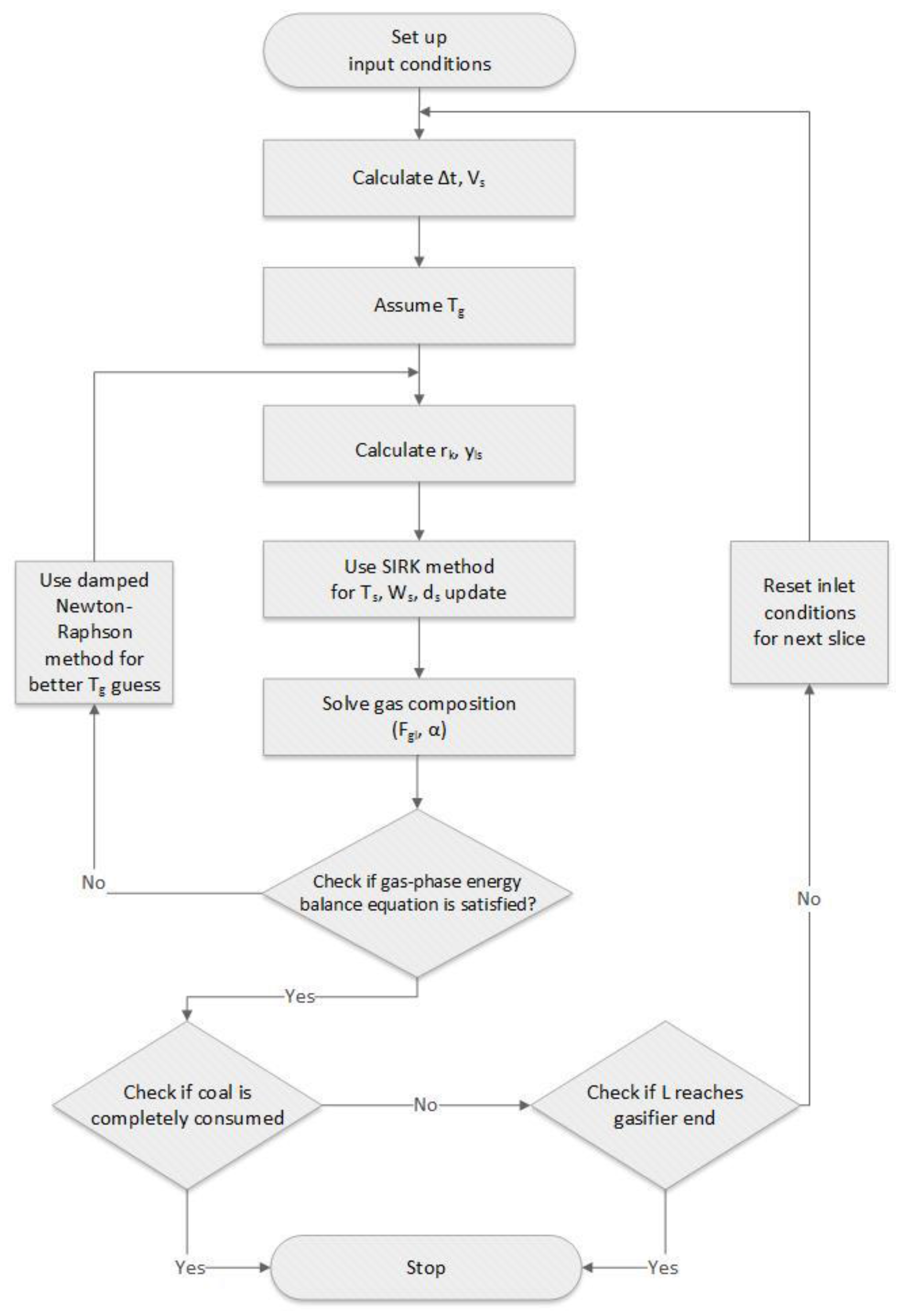
2.2.4. Solution Techniques

A time-efficient semi-implicit Runge–Kutta (SIRK) method with an algorithm of variable step size was used to solve the differential equations of mass and energy balance for a solid-phase particle [24]. A full-step half-step technique was used for the step size adjustment. This algorithm is able to increase the length of the step size whenever the difference between the exact and numerical solutions is less than the prescribed tolerance. The tolerance was 0.1 for convergence check of solid phase temperature, while it was 0.5 for convergence check of gas phase temperature. At the same time, it diminishes the computational time and improves the precision of the model [25]. An appropriate non-linear solver was used to solve the system of algebraic equations for the mass and energy balance of the gas-phase components. Figure 2 presents the computational flow diagram of the calculation procedures. The key steps to solving the above equations for each cell are described as below:

(1)

Calculate solid residence time ($\Delta t$) and solid particle velocity (V_s) using Equations (9)–(11)

(2)

Assume a value of gas temperature (T_g) at the outlet of the first cell.

(3)

Calculate the feeding rate, diameter, and temperature of a solid-phase particle from Equations (1), (2) and (7) by the SIRK method. During the calculation, each reaction rate and the mole fractions of the reactants involved in the heterogeneous reactions were calculated from Equations (3) and (4).

(4)

Calculate the molar flow rates and reaction extent of the gaseous components from Equations (5) and (6).

(5)

Update the gas temperature in Equation (8) by the damped Newton–Raphson method.

(6)

If the difference of the gas temperatures meets prescribed error tolerance, start the calculations of the next cell. Otherwise, go back to step (1) and repeat the procedure.

There are some improvements in modeling technique for simulating the gasification. In the viewpoint of modeling technique we developed for ourselves instead of commercial software, we applied semi-implicit Runge-Kutta scheme to obtain fast solution in more robust manner. In addition, we used equilibrium approach for gas phase reaction, in combination with kinetics approach for solid phase reaction. This is different from other previous work by Wen and Govind et al.

Figure 2. Computational flow of the solution procedure for the present model.

Figure 2. Computational flow of the solution procedure for the present model.

2.3. Gasifying Conditions

The key properties of coal used in the present study are given in Table 3. The experimental data by Robin [26,27] from the Texaco pilot plant gasifier was simulated by Wen et al. [9]. Those experimental and simulation data were used to validate the present model. Among several available feedstocks, coal liquefaction residue was used, whose properties are listed in Table 3.

Table 4 provides the gasifying conditions used for both the present simulation and Robin’s experiment. The baseline condition was an oxygen/coal ratio of 0.86 and a steam/coal ratio of 0.24, which are similar conditions to the coal liquefaction residue in Robin’s experiment. For the parameter studies, the oxygen/coal ratio was extended between 0.6 and 0.9, while the steam/coal ratio was extended between 0.2 and 0.8. In Wen’s work(test case), it is not clear which coal feed rate and size was used in the calculation. Here, nominal value was listed in the Table 4. Furthermore, compared to 150 μm coal used in Wen’s work, the coal size of 41 μm in this work is much closer to the ranges actually used in current industrial gasifiers. These are the same as used in Vamvuka et al. It is valuable to see the comparable results of current model with the test case using more practical input conditions.

Table 3. Key properties of coal used for comparison with Robin’s experiment [9,26].

Fuel Analysis, wt %	Coal in the Present Study	Coal Liquefaction Residue in the Robin’s Experiment, Simulated by Wen et al. [9,26]
C	74.0	74.0
H	6.2	6.2
O	1.3	1.3
N	0.7	0.7
S	1.7	1.7
Ash	16.1	16.1
Moisture	0	0

Table 3. Key properties of coal used for comparison with Robin’s experiment [9,26].

Fuel Analysis, wt %	Coal in the Present Study	Coal Liquefaction Residue in the Robin’s Experiment, Simulated by Wen et al. [9,26]
C	74.0	74.0
H	6.2	6.2
O	1.3	1.3
N	0.7	0.7
S	1.7	1.7
Ash	16.1	16.1
Moisture	0	0

Table 4. Gasifying conditions used in present simulation and Robin’s experiment [9,26].

Operating Parameters	Present Simulation	Robin’s Experiment Simulated by Wen et al.
Coal feed rate (g/s)	50	75
Coal size (μm)	41	150
Solid velocity (m/s)	0.5	0.5
Steam/coal ratio (g/g)	0.24 (0.2–0.8) *	0.24 (0.2–0.8) *
Oxygen/coal ratio (g/g)	0.86 (0.6–0.9) *	0.86 (0.6–0.9) *
Feed gas/solid temperature (K)	900	900
Gasifier pressure (MPa)	2	2
Gasifier internal diameter (cm)	150	150
Gasifier wall temperature (K)	constant	variable

* extended condition for parametric study.

Table 4. Gasifying conditions used in present simulation and Robin’s experiment [9,26].

Operating Parameters	Present Simulation	Robin’s Experiment Simulated by Wen et al.
Coal feed rate (g/s)	50	75
Coal size (μm)	41	150
Solid velocity (m/s)	0.5	0.5
Steam/coal ratio (g/g)	0.24 (0.2–0.8) *	0.24 (0.2–0.8) *
Oxygen/coal ratio (g/g)	0.86 (0.6–0.9) *	0.86 (0.6–0.9) *
Feed gas/solid temperature (K)	900	900
Gasifier pressure (MPa)	2	2
Gasifier internal diameter (cm)	150	150
Gasifier wall temperature (K)	constant	variable

* extended condition for parametric study.

In this work, the difference between the model and the experiment was minimized by adjusting several parameters. These parameters include the reaction rate of the solid-phase reaction and the wall temperature. Those could significantly affect the heat loss terms prevalent at the coal gasification/reduction zone. In the modeling work of Wen [9], key parameters governing the gasification process appear to be the wall temperature and the rate of the gas-phase reaction. Notably, the wall temperature decreased linearly as a function of reactor length. In this study, wall temperature was assumed to be constant as seen in Table 4. However, the heat generation from rate of the gaseous reaction did not affect heat loss and thus temperature profiles. This refinement was not done here since the extent of the gas reaction was determined entirely by equilibrium. Instead, the rate of solid-phase reaction was controlled in this work. Both Wen and Govind et al., considered additional heat loss in the gas phase of the combustion zone. The loss was assumed to be 30% of the total heat generated by the gaseous reactions, which we also used in this study.

Thermodynamic properties such as absolute enthalpy, entropy, and specific heat capacity at constant pressure usually vary with temperature. Values for those properties were calculated from multi-order polynomials available in NASA’s technical memorandum 4513 [28] and Chase’s paper [29]. Property data was available for the gaseous component, but not for coal of different compositions. The data for pure carbon was substituted for coal. The formation enthalpy of coal was added to the enthalpy of pure carbon to provide the absolute enthalpy of coal. The heat release (i.e., the change of enthalpy) from gas-phase and solid-phase reactions in Equations (7) and (8) was calculated by using the enthalpy data at the appropriate temperature. The change of Gibbs free energy was used as equilibrium constant in Equation (6). The transport properties of the gaseous component, such as the diffusion coefficient and thermal conductivity, were evaluated by the relationship described in Turns’s textbook [30]. Those are listed in Table 5.

Table 5. Transport properties of the gaseous component used in this simulation.

Properties	Relations
Diffusion coefficient (m2/s)	$D_{O_2-N_2}={\left(\frac{T_g}{393}\right)}^{1.5}\cdot \left(\frac{1}{p}\right)\cdot 1.6\times {10}^{-5}$
	$D_{C{O}_2-N_2}={\left(\frac{T_g}{393}\right)}^{1.5}\cdot \left(\frac{1}{p}\right)\cdot 1.6\times {10}^{-5}$
	$D_{H_{2}O-air}={\left(\frac{T_g}{273}\right)}^{1.5}\cdot \left(\frac{1}{p}\right)\cdot 2.2\times {10}^{-5}$
	$D_{H_2-air}={\left(\frac{T_g}{273}\right)}^{1.5}\cdot \left(\frac{1}{p}\right)\cdot 0.61\times {10}^{-5}$
Thermal conductivity (J/m-s-K)	$\mathsf{\lambda }=0.113$ at 1700 K

Table 5. Transport properties of the gaseous component used in this simulation.

Properties	Relations
Diffusion coefficient (m2/s)	$D_{O_2-N_2}={\left(\frac{T_g}{393}\right)}^{1.5}\cdot \left(\frac{1}{p}\right)\cdot 1.6\times {10}^{-5}$
	$D_{C{O}_2-N_2}={\left(\frac{T_g}{393}\right)}^{1.5}\cdot \left(\frac{1}{p}\right)\cdot 1.6\times {10}^{-5}$
	$D_{H_{2}O-air}={\left(\frac{T_g}{273}\right)}^{1.5}\cdot \left(\frac{1}{p}\right)\cdot 2.2\times {10}^{-5}$
	$D_{H_2-air}={\left(\frac{T_g}{273}\right)}^{1.5}\cdot \left(\frac{1}{p}\right)\cdot 0.61\times {10}^{-5}$
Thermal conductivity (J/m-s-K)	$\mathsf{\lambda }=0.113$ at 1700 K

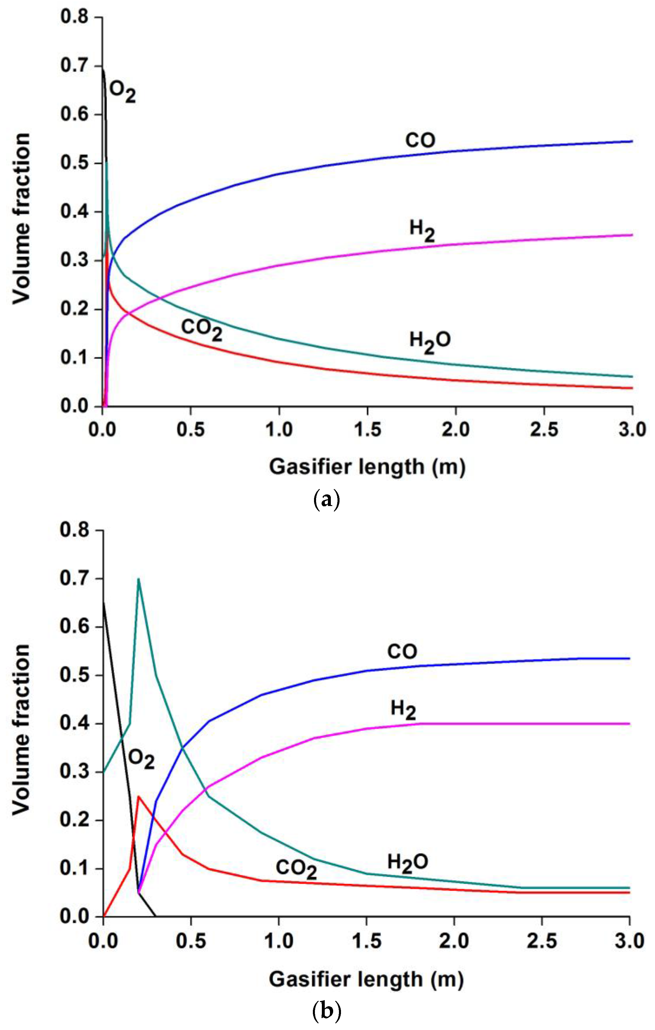
3. Results and Discussion

3.1. Model Prediction and Validation

Owing to experimental difficulties, few experiments are available on the entrained flow gasifier in the literature. Among them, the Texaco downflow entrainment pilot plant was developed by Robin [24,25]. He evaluated various feedstocks, including coal liquefaction residues and coal-water mixture. The experimental results were simulated by both Wen and Govind. They also predicted gasifier performance under additional operating conditions, expanded from the standard condition of the original design. Vamvuka and Woodburn also simulated gasifier performance at operating conditions similar to the Texaco gasifier, but did not compare their results against experiments [13].

Other experimental results for pressurized entrained flow reactors were reported by Hla et al. [31]. Gasification behaviors were evaluated for different coal types. However, the maximum flow rate of the coal was limited to 1.4 g/s, and the oxidant was air, which was diluted by nitrogen. Therefore, the peak temperatures of the gas and solid phases, and the gas composition, were lower than those of actual gasifiers. In addition, there was no information on the effect of the steam/coal ratio on the performance.

For these reasons, the experimental and simulated results from the Texaco gasifier were used in order to demonstrate the current model’s validity. Figure 3 presents profiles of gas composition on a wet basis, from both the present model and Wen’s model. The operating conditions were comparable, with an O₂/fuel ratio = 0.8 and an H₂O/fuel ratio = 0.2. There is moderate agreement for the distribution of the major product gases (CO, H₂, and CO₂) between the computed and the experimental data along the length of the reactor. Steam and CO₂ concentrations attain a maximum at a position where oxygen is completely consumed [10]. There is a discrepancy in the position of oxygen consumption indicating the onset of combustion. The composition of the dry product gas at the outlet is compared in Table 6. They are clearly in marked agreement.

Table 6. Major product gas composition (on a dry basis) at the outlet for the present model and Wen’s model [9] at standard condition.

Gas Composition (vol %, Dry Basis)	Computed Result from Present Model	Robin’s Experiment Simulated by Wen et al.
CO2	4.8	4.1
CO	54.6	54.0
H2	40.5	41.0

Table 6. Major product gas composition (on a dry basis) at the outlet for the present model and Wen’s model [9] at standard condition.

Gas Composition (vol %, Dry Basis)	Computed Result from Present Model	Robin’s Experiment Simulated by Wen et al.
CO2	4.8	4.1
CO	54.6	54.0
H2	40.5	41.0

Figure 3. Calculated product gas composition profiles (on a wet basis) at an O₂/fuel ratio = 0.86 and an H₂O/fuel ratio = 0.24 from (a) the present model and (b) Wen’s model [9].

Figure 3. Calculated product gas composition profiles (on a wet basis) at an O₂/fuel ratio = 0.86 and an H₂O/fuel ratio = 0.24 from (a) the present model and (b) Wen’s model [9].

More composition data is compared for different stoichiometric conditions as available in the next Figure 5. Although it is not shown here, the gas and solid particles reach a maximum temperature at 2300 K and 2170 K, respectively, because of the heat release from the combustion reactions in the solid and gas phases. After this point, temperatures decrease since the heat loss to the wall and the endothermic solid reactions become more involved.

In Figure 4, a second evaluation of the differences between present model and Wen’s model was made in terms of carbon conversion under various operating conditions of oxygen and steam/fuel ratios. The computed results from the current model were consistent with those from Wen’s model. Remarkably, two important behaviors were found for both calculations. First, the oxygen/fuel ratio appears to affect carbon conversion more significantly than the steam/fuel ratio. This behavior is attributed to the fact that the heat produced from the combustion reactions supports the subsequent gasification reactions. However, further increase in the oxygen/fuel ratio beyond 0.8 is not effective in continuing to increase carbon conversion. For example, the present model showed that 90%–99% of the carbon was converted at an oxygen/fuel ratio between 0.75 and 0.9. This trend is similar to one from the measurement in the Texaco pilot plant [26,27], and from the experimental work of Watanabe et al. [32,33].

Figure 4. Distribution of carbon conversion from (a) the present model and (b) Wen’s model [9].

Figure 4. Distribution of carbon conversion from (a) the present model and (b) Wen’s model [9].

At low oxygen/coal ratios, the optimal range of the steam/coal ratio for maximizing carbon conversion is 0.3–0.5. This second trend is present in both the present results and in Wen’s results. As the steam/fuel ratio increases, it promotes the coal-steam reaction, thus increasing carbon conversion because of high reactant availability. In parallel, the presence of the WGS reaction increases other reactants such as CO₂, which promotes the coal-CO₂ reaction, thus increasing carbon conversion. However, the carbon conversion turns into a reduction as the steam/fuel ratio increases further. This reduction is caused by two mechanisms: First, heat loss becomes pronounced lowering the reaction temperature, since both the char-steam and the char-CO₂ reactions are highly endothermic through the interaction term between the gas phase and the solid phase. This reduced temperature in turn lowers the gasification rate of the solid particles and carbon conversion. Second, a greater amount of steam and CO₂ in the product absorbs the heat release from the reaction, in turn reducing the reaction temperature. As a result, the reduced temperature lowers the gasification rate and carbon conversion. Other terms are small compared with the heat storage term in Equation (8), including heat release from the gaseous reactions and heat loss to the wall. As a brief summary, both reaction temperature and steam-CO₂ concentration affect carbon conversion, resulting in an optimum steam/fuel ratio at a fixed oxygen/fuel ratio. Those effects are discussed further in the section titled “Mechanism of CO variation between reactor model and equilibrium model”. However, the presence of optimal carbon conversion was not observed in the numerical results of Vamvuka [13].

In Figure 5a, the major gas composition from the present model is compared against Wen’s model. The data were shown on a dry basis as a function of the oxygen/fuel ratio at a constant steam/fuel ratio. There is a turning point for the hydrogen and CO₂ in the product gases around 0.8 as the oxygen/fuel ratio increases. In Wen’s work, this inflection was attributed to competition between coal-oxygen, coal-CO₂, coal-steam, and the WGS gas reaction [9]. Figure 5b shows the effect of the steam/fuel ratio on the product gas composition at a constant oxygen/fuel ratio (=0.86). As the steam/fuel ratio increases, the fraction of CO in the product gas decreases, while those of CO₂ and H₂ increase. This effect of the steam/fuel ratio on the gas product distribution is more significant, as compared to the oxygen-fuel effect discussed above. The agreement between the two models was reasonable, despite some differences in operating conditions as mentioned earlier. These findings are also consistent with those reported by Vamvuka et al., where the magnitude of CO₂ is overestimated for comparable conditions [13]. This difference may be because of either the WGS dominance at reduced temperatures or the weaker solid reaction in the work of Vamvuka.

Figure 5. Major gas composition of the present model and Wen’s model [9] on a dry basis as function of (a) oxygen/fuel ratio at similar steam/fuel ratio = 0.24 and (b) steam/fuel ratio at similar oxygen/fuel ratio = 0.86.

Figure 5. Major gas composition of the present model and Wen’s model [9] on a dry basis as function of (a) oxygen/fuel ratio at similar steam/fuel ratio = 0.24 and (b) steam/fuel ratio at similar oxygen/fuel ratio = 0.86.

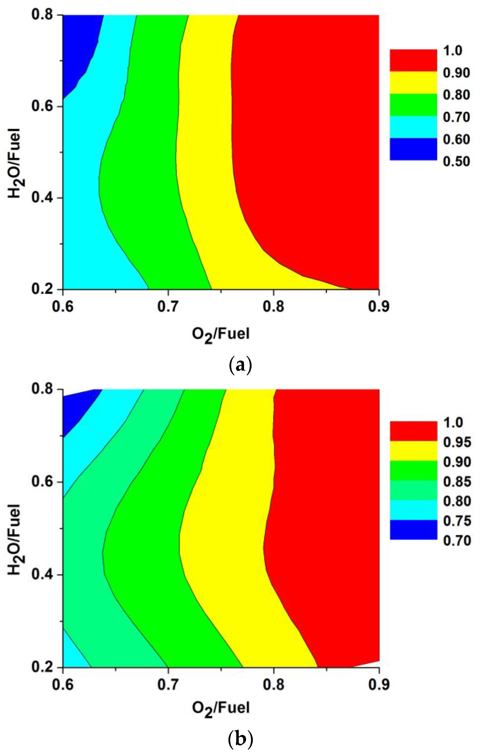
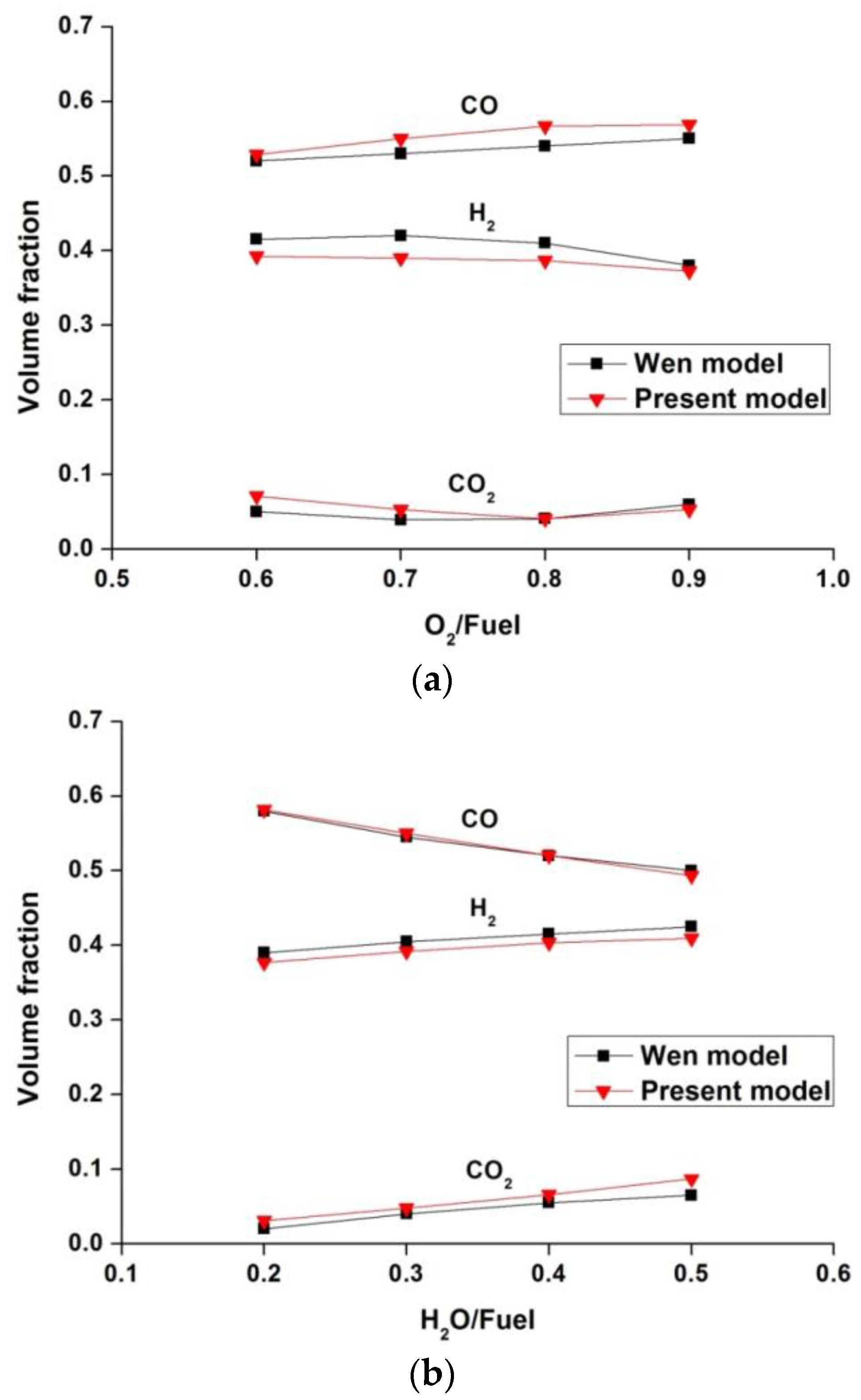
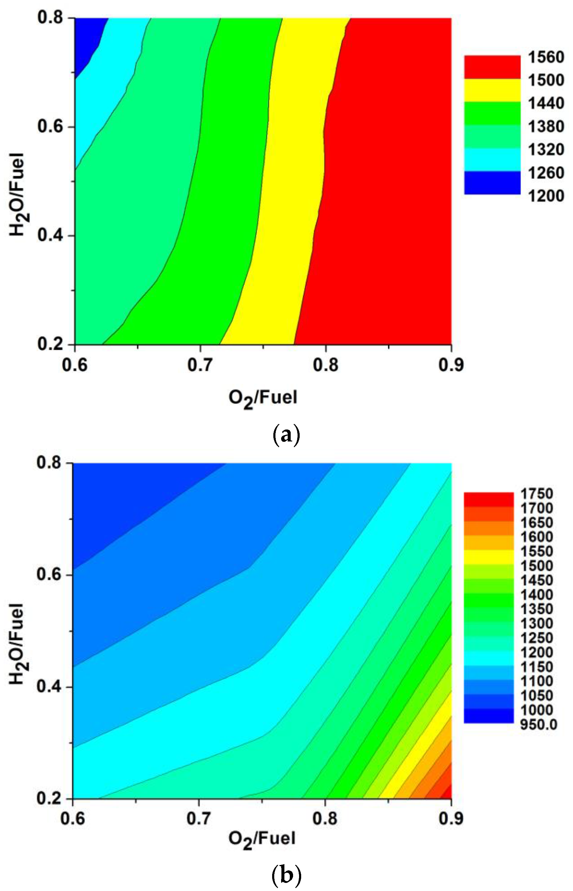
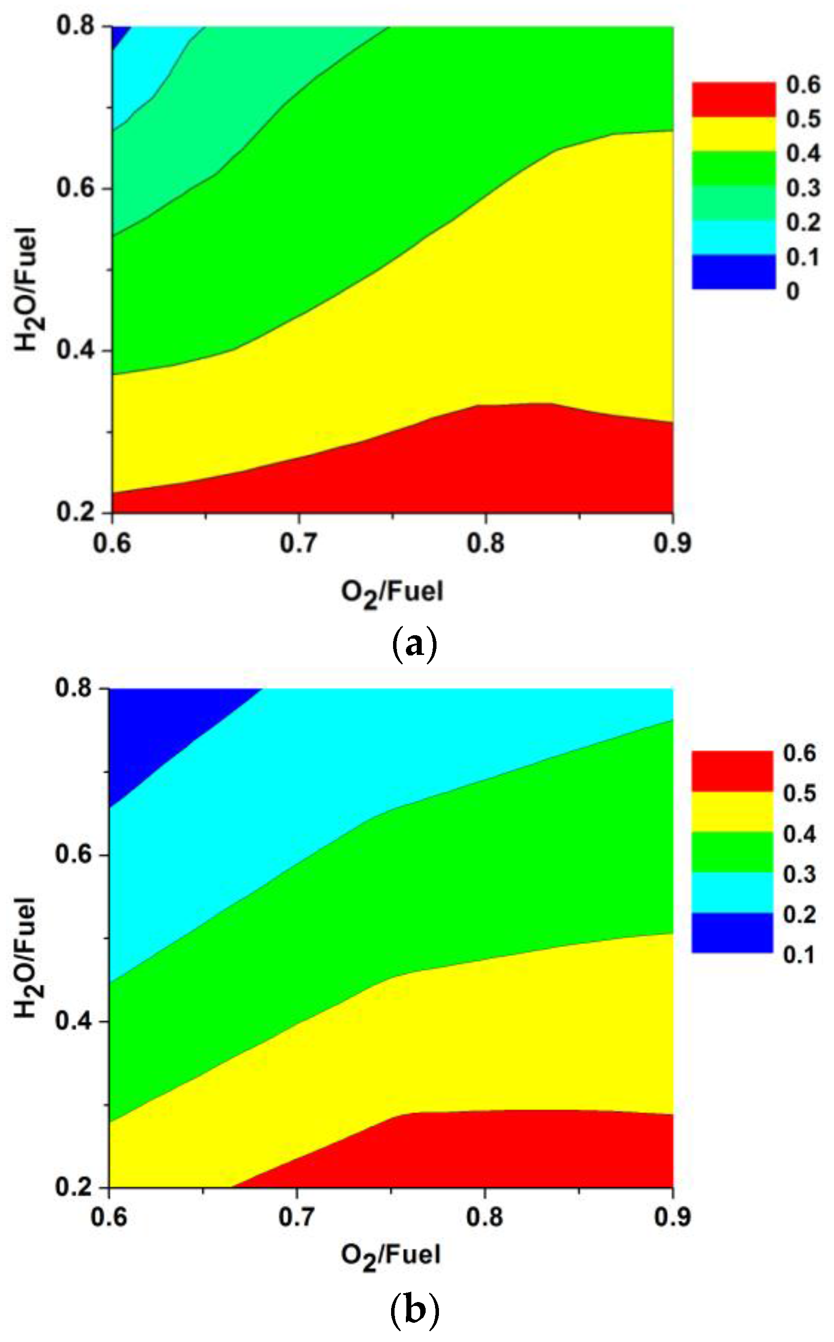
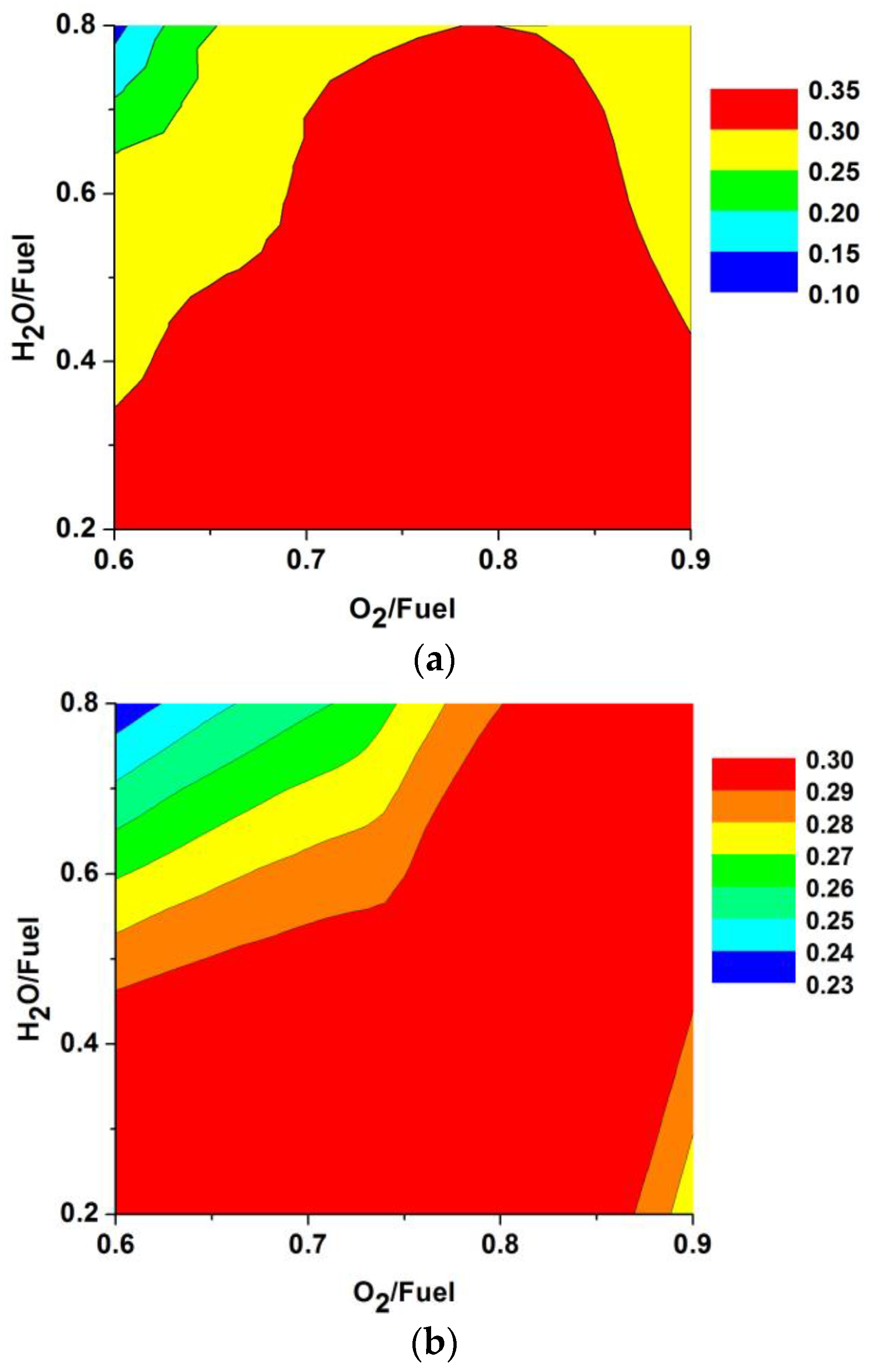
3.2. Comparison with Equilibrium Model

Further parameter studies of the present model were made to provide a better understanding of reactor performance for various operating conditions. Those data were compared against the predicted results from the two-phase equilibrium model [34,35]. The equilibrium solution was obtained by using the open source software, Cantera. Inside the Cantera, two-phase approach to account for carbon reactions in solid phase was implemented. The details about the equilibrium model and solution are found in the previous work of the authors [36]. In the past, there were no detailed studies examining the differences between the equilibrium model and the reactor model, particularly at various gasifying conditions. The coal properties and gasifying conditions are the same as the previous coal values used for validating reactor model in Table 3 and Table 4, respectively. Biagini et al., compared their reactor model results with equilibrium results [37]. The equilibrium results did not provide good agreement with their reactor model. Those are attributed to several different factors including isothermal condition where reaction temperature is known.

Figure 6 presents the distribution of CO concentration on a wet basis for various ranges of the oxygen/coal and steam/coal ratios. The computed results from the present reactor model were compared with results from the two-phase equilibrium model. As the oxygen/fuel ratio increases, CO increases because of the increased temperature. The temperature rise results in the conditions in which gaseous reactions such as the WGS or CH₄ formation are suppressed, or carbon conversion from the solid reaction increases. As discussed more in a later section, one effect may dominate another, depending on whether the equilibrium model or the reactor model are used. For an oxygen/fuel ratio beyond 0.8, CO decreases since abundant oxygen promotes CO₂ formation. As the steam/fuel ratio increases, CO decreases owing to reduced temperature and reduced WGS reactions. Those behaviors are observed in both models, which show negligible differences in the peak value and position.

Figure 6. Distribution of CO concentration (on a wet basis) for various ranges of oxygen/coal ratio and steam/coal ratio, computed from (a) from the present reactor model and (b) the two-phase equilibrium model.

Figure 6. Distribution of CO concentration (on a wet basis) for various ranges of oxygen/coal ratio and steam/coal ratio, computed from (a) from the present reactor model and (b) the two-phase equilibrium model.

Figure 7 presents the distribution of H₂ concentration for various ranges of oxygen/coal and steam/coal ratios, computed from (a) the present reactor model and (b) the two-phase equilibrium model. The H₂ contour differs greatly from those of CO and CO₂ concentration as shown above. In the ranges of interest, no inflection trend for H₂ concentration was found at critical steam/coal ratios lower than 0.4. The trend is quite similar for the two models. Rather, the H₂ appears to remain unchanged as the oxygen/coal ratio decreases from 0.9. In the case of the equilibrium calculation, this behavior was caused by two competitions: carbon conversion from solid reactions and concurrent gaseous reactions. From the thermodynamic viewpoint, both reactions occur predominantly at reduced temperatures [34]. The strong dependence of hydrogen content on solid carbon conversion is in line with the experimental data of Jarungthammachote et al. [5]. Strong agreement was observed between the experiment and the simulation when the carbon conversion effect was considered in the model. Melgar et al., reported measured data for a biomass downdraft gasifier where hydrogen content was kept constant when the oxygen/coal ratio was less than 0.75 [35]. Bockelie et al., demonstrated a distribution of hydrogen concentration much closer to that in the equilibrium calculation [38]. Similar variation of hydrogen with oxygen/coal ratio was observed in Hla’s simulation [39].

Figure 7. Distribution of H₂ concentration (for a wet basis) for various ranges of oxygen/coal ratio and steam/coal ratio, computed from (a) the present reactor model and (b) the two-phase equilibrium model.

Figure 7. Distribution of H₂ concentration (for a wet basis) for various ranges of oxygen/coal ratio and steam/coal ratio, computed from (a) the present reactor model and (b) the two-phase equilibrium model.

On the contrary, there were equilibrium results in which the solid carbon reaction was not considered in the calculation. There was an island of hydrogen concentration corresponding to a peak value. The inflection occurs with increasing oxygen/fuel ratios at constant steam/coal ratios lower than 0.4. For instance, H₂ decreased caused by CO methanation at low temperatures as the oxygen/coal ratio decreased on the left of the island. In contrast, H₂ decreased as the oxygen/coal ratio increased on the right of the island. The hydrogen in the coal converts to H₂O, rather than H₂ owing to suppression of the WGS at high temperatures. Therefore, this was explained by two gaseous reactions (i.e., CO methanation and WGS) and by temperature. These mechanisms were completely described in the numerical work of Caton et al. [40].

In Figure 8, the two models were compared in terms of cold gas efficiency at various conditions. The cold gas efficiency designates the amount of heat generated from the combustion reaction of the product gases with respect to the initial chemical energy of coal. Specifically, a sum of the lower heating values (LHV) of the product gases was divided by the lower heating value of the coal feed to the gasifier. The maximum value of cold gas efficiency was observed for the reactor model at the oxygen/fuel ratio of 0.8 with less dependence on steam/fuel ratios. This was expected as the maximum amounts of CO and H₂ were observed around it. The cold gas efficiency appears to be influenced mainly by the oxygen/fuel ratio, rather than the steam/fuel ratio. These behaviors were observed for the equilibrium results as well. As a result, an oxygen/coal ratio of 0.8 and a steam/coal ratio of 0.4 are the optimal condition, at which both carbon conversion and cold gas efficiency are considered by priority. From the practical viewpoint of operating a wet-feed gasifier, a realistic limit of the steam/fuel ratio is determined by other factors such as coal loading. Coal loading below 70%, which roughly corresponds to a steam/fuel ratio greater than 0.4, is acceptable.

Figure 8. Distribution of cold gas efficiency for various ranges of oxygen/coal ratio and steam/coal ratio, computed from (a) the present reactor model and (b) the two-phase equilibrium model.

Figure 8. Distribution of cold gas efficiency for various ranges of oxygen/coal ratio and steam/coal ratio, computed from (a) the present reactor model and (b) the two-phase equilibrium model.

3.3. Mechanism of CO Variation between Reactor Model and Equilibrium Model

As discussed with Figure 6, there are two ways to vary CO concentration as a function of the oxygen/fuel ratio. As the oxygen/fuel ratio decreases from 0.8, temperature decreases. When the temperature is below 1200 K, gaseous reactions such as the WGS or CH₄ formation become more favorable. This is the dominant mechanism governing CO reduction in the equilibrium model. Likewise, this mechanism appears to be responsible for the CO decrease observed as a function of the steam/fuel ratio. In contrast, solid reactions could affect CO concentration in another way. When temperature does not drop below 1200 K, CO reduction is caused by the decreasing level of solid reactions, as the oxygen/fuel ratio decreases from 0.8. This is the prevalent mechanism in the present reactor model.

Those mechanisms are supported by the temperature distribution of Figure 9. A time-weighted (or averaged) gas temperature was calculated at the outlet from the present reactor model. Meanwhile, the temperature at the outlet was computed from the equilibrium model. The decreasing temperature trend with the decreasing oxygen/fuel ratio was present for both models. In the case of the reactor model, the final temperature was determined by both heat loss and generation in energy balance Equation (8), as discussed previously for carbon conversion. The comparison shows that the temperature of the reactor model is much higher than that of the equilibrium model. The reactor temperature ranges well over 1200 K under most conditions. The changes in the reactor model with the decreasing oxygen/fuel ratio are less than those in the equilibrium model. Therefore, gaseous reactions such as the WGS and CH₄ formation were not strong enough to affect CO concentration. Instead, solid reactions affected CO concentration significantly. This mechanism was also responsible for the CO decrease observed when the steam/coal ratio increases.

Figure 9. Distribution of time-weighted gas temperature for various ranges of oxygen/coal ratio and steam/coal ratio, computed from (a) the present reactor model and (b) the two-phase equilibrium model.

Figure 9. Distribution of time-weighted gas temperature for various ranges of oxygen/coal ratio and steam/coal ratio, computed from (a) the present reactor model and (b) the two-phase equilibrium model.

4. Conclusions

In this study, a steady-state reactor model was developed for the entrained flow coal gasification process. The computational results from the present reactor model were validated against experimental data. Further parameter studies of the present reactor model were made to provide a better understanding of reactor performance for various operating conditions. Those data were compared with those from the two-phase equilibrium model we developed previously. The dominant mechanisms governing product gas composition was discussed for both models.

The results show that the oxygen/coal ratio affects carbon conversion more significantly than does the steam/coal ratio. The optimal range for the steam/coal ratio for maximizing carbon conversion, 0.3–0.6, is influenced by the reaction temperature and the steam-CO₂ concentration. The steam/coal ratio affects product gas composition, such as hydrogen and carbon monoxide, more significantly. There was quite reasonable agreement with the equilibrium result for major gas composition. Gaseous reactions are the dominant mechanism governing CO reduction with a reduction in the oxygen/coal ratio in the equilibrium model, while solid reactions are more significant in the reactor model. Those mechanisms were ascribed to differences in the reaction temperature between the two models.

References

1. National Energy Technology Laboratory. Integrated gasification combined cycle (IGCC) cases. In Cost and Performance Baseline for Fossil Energy Plants, Volume 3a: Low Rank Coal to Electricity; National Energy Technology Laboratory: Morgantown, WV, USA, 2011. [Google Scholar]
2. National Energy Technology Laboratory. Cost and Performance Baseline for Fossil Energy Plants, Volume 2: Coal to Synthetic Natural Gas and Ammonia; National Energy Technology Laboratory: Morgantown, WV, USA, 2011.
3. Chen, C.; Horio, M.; Kojima, T. Numerical simulation of entrained flow coal gasifiers. Part II: Effects of operating conditions on gasifier performance. Chem. Eng. Sci. 2000, 55, 3875–3883. [Google Scholar] [CrossRef]
4. Chen, C.; Horio, M.; Kojima, T. Numerical simulation of entrained flow coal gasifiers, Part I: Modeling of coal gasification in an entrained flow gasifier. Chem. Eng. Sci. 2000, 55, 3861–3874. [Google Scholar] [CrossRef]
5. Jarungthammachote, S.; Dutta, A. Equilibrium modeling of gasification: Gibbs free energy minimization approach and its application to spouted bed and spout-fluid bed gasifiers. Energy Convers. Manag. 2008, 49, 1345–1356. [Google Scholar] [CrossRef]
6. Baratieri, M.; Baggio, P.; Fiori, L.; Grigiante, M. Biomass as an energy source: Thermodynamic constraints on the performance of the conversion process. Bioresour. Technol. 2008, 99, 7063–7073. [Google Scholar] [CrossRef] [PubMed]
7. Rodolfo, R.; Nilson, R.M.; Jorge, O.T.; Marcelo, G.; Adriene, M.S.P. Co-gasification of footwear leather waste and high ash coal: A thermodynamic analysis. In Proceedings of the 27th Annual International Pittsburgh Coal Conference, Turkey, Istanbul, 11–14 October 2010.
8. Ubhayakar, S.K.; Stickler, D.B.; Gannon, R.E. Modelling of entrained bed pulverized coal gasifiers. Fuel 1977, 56, 281–291. [Google Scholar] [CrossRef]
9. Wen, C.Y.; Chaung, T.Z. Entrainment coal gasification modeling. Ind. Eng. Chem. Process. Des. Dev. 1979, 18, 684–695. [Google Scholar] [CrossRef]
10. Govind, R.; Shah, J. Modeling and simulation of an entrained flow coal gasifier. AIChE J. 1984, 30, 79–92. [Google Scholar] [CrossRef]
11. Zhao, W.; Ding, Y.; Liu, Z.; Wu, Z. Modeling for an entrained flow coal gasifier with partitioning zone approach. In Proceedings of the 7th World Congress on Intelligent Control and Automation, Chongqing, China, 25–27 June 2008.
12. Vamvuka, D.; Woodburn, E.T.; Senior, P.R. Modelling of an entrained flow coal gasifier: 1. Development of the model and general predictions. Fuel 1995, 74, 1452–1460. [Google Scholar] [CrossRef]
13. Vamvuka, D.; Woodburn, E.T.; Senior, P.R. Modeling of an entrained flow coal gasifier: 2. Effect of operating conditions on reactor performance. Fuel 1995, 74, 1461–1465. [Google Scholar] [CrossRef]
14. Shahrivar, H.H.; Sheikhi, A.; Sotudeh-Gharebagh, R. On the flow direction effect in sequential modular simulations: A case study on fluidized bed biomass gasifiers. Int. J. Hydrog. Energy 2015, 40, 2552–2567. [Google Scholar] [CrossRef]
15. Sohi, A.H.; Eslami, A.; Sheikhi, A.; Sotudeh-Gharebagh, R. Sequential-based process modeling of natural gas combustion in a fluidized bed reactor. Energy Fuels 2012, 26, 2058–2067. [Google Scholar] [CrossRef]
16. Asadi-Saghandi, H.; Sheikhi, A.; Sotudeh-Gharebagh, R. Sequence-based process modeling of fluidized bed biomass gasification. ACS Sustain. Chem. Eng. 2015, 3, 2640–2651. [Google Scholar] [CrossRef]
17. Eslami, A.; Sohi, A.H.; Sheikhi, A.; Sotudeh-Gharebagh, R. Sequential modeling of coal volatile combustion in fluidized bed reactors. Energy Fuels 2012, 26, 5199–5209. [Google Scholar] [CrossRef]
18. Badzioch, S.; Hawksley, P.B.W. Kinetics of thermal decomposition of pulverized coal particles. Ind. Eng. Chem. Process. Dev. 1970, 9, 521–530. [Google Scholar] [CrossRef]
19. Kane, R.S.; McCailister, R.A. Scaling laws and differential equations of an entrained flow coal gasifier. AIChE J. 1978, 24, 55–63. [Google Scholar] [CrossRef]
20. Von Fredersdorff, C.G.; Elliott, M.A. Chemistry of Coal Utilization, Supplementary Volume; Lowry, H.H., Ed.; Wiley: New York, NY, USA, 1963. [Google Scholar]
21. Kajitani, S.; Suzuki, N.; Ashizawa, M.; Hara, S. CO2 gasification rate analysis of coal char in entrained flow coal gasifier. Fuel 2006, 85, 163–169. [Google Scholar] [CrossRef]
22. Blasi, C.D. Dynamic behaviour of stratified downdraft gasifiers. Chem. Eng. Sci. 2000, 55, 2931–2944. [Google Scholar] [CrossRef]
23. Laurendeau, N.M. Progress in energy and combustion science. Prog. Energy Combust. Sci. 1978, 4, 221–270. [Google Scholar] [CrossRef]
24. Davis, M.E. Numerical Methods and Modelling for Chemical Engineers; John Wiley & Sons: New York, NY, USA, 1984. [Google Scholar]
25. Adanez, J.; Labiano, F.G. Modeling of moving-bed coal gasifiers. Ind. Eng. Chem. Res. 1990, 29, 2079–2088. [Google Scholar] [CrossRef]
26. Robin, A.M. Hydrogen Production from Coal Liquefaction Residues; Electric Power Research Institute (EPRI) Report: El monte, CA, USA, 1976. [Google Scholar]
27. Robin, A.M. Gasification of Residual Materials from Coal Liquefaction; Department of Energy (DOE) Report: El Monte, CA, USA, 1977. [Google Scholar]
28. McBride, B.J.; Gordon, S.; Reno, M.A. NASA Technical Memorandum 4513; NASA Report: Cleveland, OH, USA, 1980. [Google Scholar]
29. Chase, M.W. NIST-JANAF Thermochemical Tables, 4th ed.; J. Phys Chem Ref Data, Monograph 9; American Chemical Society: New York, NY, USA, 1998. [Google Scholar]
30. Turns, S.R. Introduction to Combustion: Concepts and Applications, 2nd ed.; McGraw Hills: New York, NY, USA, 2000. [Google Scholar]
31. Hla, S.S.; Haris, D.; Roberts, D. Gasification Conversion Model: PEFR; Research Report 80; Commonwealth Scientific and Industrial Research Organization (CSIRO): Sydney, Austrailia, 2007. [Google Scholar]
32. Watanabe, H.; Otaka, M. Numerical simulation of coal gasification in entrained flow coal gasifier. Fuel 2006, 85, 1935–1943. [Google Scholar] [CrossRef]
33. Zainal, Z.A.; Rifau, A.; Quadir, G.A.; Seetharamu, K.N. Experimental investigation of a downdraft biomass gasifier. Biomass Bioenergy 2002, 23, 283–289. [Google Scholar] [CrossRef]
34. Baggio, P.; Baratieri, M.; Fiori, L.; Grigiante, M.; Avi, D.; Tosi, P. Experimental and modeling analysis of a batch gasification/pyrolysis reactor. Energy Convers. Manag. 2009, 50, 1426–1435. [Google Scholar] [CrossRef]
35. Melgar, A.; Perez, J.F.; Laget, H.; Horillo, A. Thermochemical equilibrium modelling of a gasifying process. Energy Convers. Manag. 2007, 48, 59–67. [Google Scholar] [CrossRef]
36. Hwang, M.K.; Kim, M.S.; Lee, S.C.; Kim, K.B.; Boehman, A.L.; Song, J.H. Simulation of a coal gasifier at different bed conditions. AIME 2015. submitted. [Google Scholar]
37. Biagini, E.; Bardi, A.; Pannocchia, G.; Tognotti, L. Development of an entrained flow gasifier model for process optimization study. Ind. Eng. Chem. Res. 2009, 48, 9028–9033. [Google Scholar] [CrossRef]
38. Bockelie, M.J.; Denison, M.K.; Chen, Z.; Senior, C.L.; Sarofim, A.F. Using models to select operating conditions for gasifiers. Reaction Engineering International. Available online: http://citeseerx.ist.psu.edu/viewdoc/download?doi=10.1.1.522.9198&rep=rep1&type=pdf (accessed on 6 May 2015).
39. Hla, S.S.; Roberts, D.G.; Harris, D.J. A numerical model for understanding the behaviour of coals in an entrained-flow gasifier. Fuel Process. Technol. 2015, 134, 424–440. [Google Scholar] [CrossRef]
40. Caton, P.A.; Carr, M.A.; Kim, S.S.; Beautyman, M.J. Energy recovery from waste food by combustion or gasification with the potential for regenerative dehydration: A case study. Energy Convers. Manag. 2010, 51, 1157–1169. [Google Scholar] [CrossRef]