Article

Performance of a Predictive Model for Calculating Ascent Time to a Target Temperature

School of Architecture and Building Science, Chung-Ang University, Seoul 06974, Korea
*
Author to whom correspondence should be addressed.
Energies 2016, 9(12), 1090; https://doi.org/10.3390/en9121090
Submission received: 7 October 2016 / Revised: 7 December 2016 / Accepted: 15 December 2016 / Published: 20 December 2016
(This article belongs to the Special Issue Smart Home Energy Management)

Abstract

:
The aim of this study was to develop an artificial neural network (ANN) prediction model for controlling building heating systems. This model was used to calculate the ascent time of indoor temperature from the setback period (when a building was not occupied) to a target setpoint temperature (when a building was occupied). The calculated ascent time was applied to determine the proper moment to start increasing the temperature from the setback temperature to reach the target temperature at an appropriate time. Three major steps were conducted: (1) model development; (2) model optimization; and (3) performance evaluation. Two software programs—Matrix Laboratory (MATLAB) and Transient Systems Simulation (TRNSYS)—were used for model development, performance tests, and numerical simulation methods. Correlation analysis between input variables and the output variable of the ANN model revealed that two input variables (current indoor air temperature and temperature difference from the target setpoint temperature), presented relatively strong relationships with the ascent time to the target setpoint temperature. These two variables were used as input neurons. Analyzing the difference between the simulated and predicted values from the ANN model provided the optimal number of hidden neurons (9), hidden layers (3), moment (0.9), and learning rate (0.9). At the study’s conclusion, the optimized model proved its prediction accuracy with acceptable errors.

1. Introduction

People are now spending around 90% of their time indoors [1]. Therefore, indoor environmental quality (IEQ) has become a significant factor for building occupants’ quality of life. Comfort, health, and productivity are affected by IEQ, and it can significantly affect occupant behavior [2]. Properly provided IEQ in commercial buildings can reduce absenteeism rates and employee turnover, and increase productivity. Better IEQ can lead to fewer errors and accidents, and improve product and service quality [3]. In addition, proper IEQ can reduce health hazards [4,5,6,7,8].
Heating and cooling systems account for 58.1% of total energy use in Korean residential buildings [9,10]. Residential thermostats allow occupants to control their setpoint timeframes and temperatures. This allows occupants to manage their personal comfort while reducing energy consumption.
A variety of building control systems using diverse types of energy have been applied to create a comfortable indoor environment. For example, heating and cooling systems, which aim to provide comfortable indoor thermal conditions, primarily account for most of the residential energy consumption. The amount of heating and cooling energy consumption reaches 58.1% of the total energy use in Korean residential buildings [9,10].
For providing comfortable thermal environment in an energy-efficient manner, a variety of theoretical and practical approaches have been studied and applied. The application of the thermostat for heating and cooling systems is one practical example that is widespread as a control method. The thermostat provides a function whereby users can determine their preferable setpoint and setback temperatures and periods. The application of thermostats is expected to provide two principal advantages: (1) improved thermal comfort; and (2) reduced energy consumption [2].
Thermal comfort should be improved for two reasons. The first reason is that the indoor thermal environment can be adjusted to the desired level, and the second reason is that occupants can be psychologically satisfied with having an opportunity to control their thermal environment. In previous studies, occupants expressed increased satisfaction when they could use a thermal control device such as the thermostat to be involved in the thermal control process [11,12,13].
In addition, using a thermostat that employs the setback temperature can save on the energy consumed for the thermal conditioning of the space. The setback temperature can be applied for the day- and nighttime for reducing energy consumption without compromising thermal comfort. In previously conducted experiments, field tests, and computer simulations, a significant energy saving effect of up to 30% for heating and 23% for cooling in residential buildings was reported [14,15,16,17,18,19]. Other types of buildings such as office buildings, hospitals, educational and religious buildings, etc. also achieved remarkable savings in energy consumption for thermal conditioning through the application of energy-conscious thermostats [20,21]. The programmable thermostat was an example of those thermostats, with which occupants could choose normal setpoint and setback temperatures and periods [22].
Advanced strategies for the optimal programming of setback temperature such as adaptive, demand response, and virtual thermostats have been introduced to maximize thermal comfort and increase energy savings [23,24,25,26]. In particular, Yang and Kim investigated a method to determine the optimal start moment of the heating system using an artificial neural network (ANN) model [27,
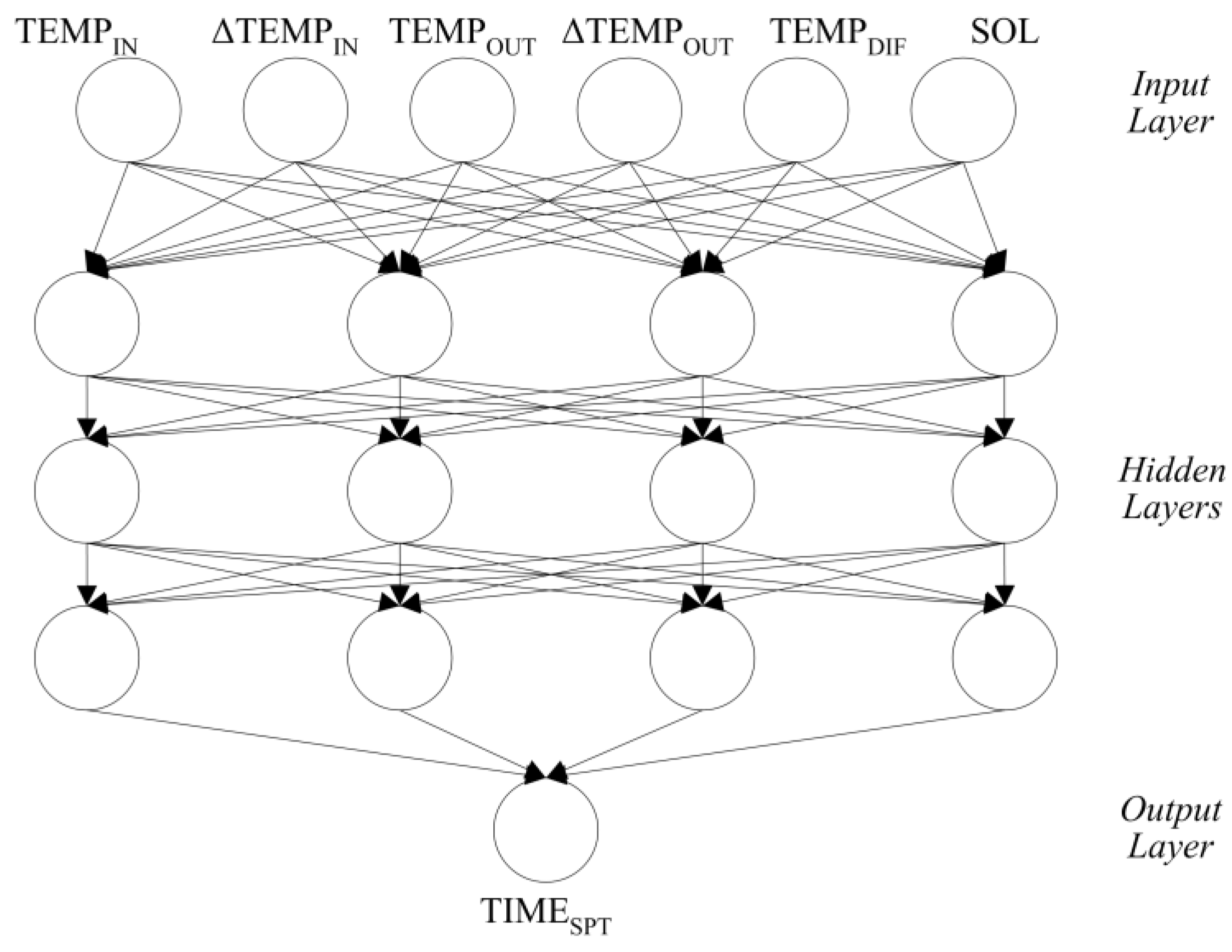
28]. The ANN model was designed to predict the required time for changing the indoor temperature to the desired temperature. Four input variables were employed as input neurons in the ANN model: indoor air temperature, varying rate of room air temperature, outdoor air temperature, and varying rate of outdoor air temperature. Model optimization was conducted for learning rate, momentum, nodes of hidden layer, and use of bias. The optimized model showed statistically meaningful prediction accuracy.
Despite the achievements of this research, two issues still need to be addressed. The first is the selection process for the input variables. In the previous study, the four input variables were selected as input neurons according to the factor analysis affecting room air temperature. However, no statistical analysis on the relationship between the input and output variables was conducted. Thus a simpler model, which excludes input variables having a lesser relationship, could be developed in further study.
The second issue is the optimization process of the model. The objective of the optimization was to find the ANN composition and learning method that would give the most accurate prediction results. For finding the optimized composition and learning method, the parameters to be optimized were tested independently and sequentially. After one factor (e.g., learning rate) was optimized, the next factor (e.g., momentum) was tested, to find the optimal value after fixing the first factor as an optimal value. Thus, an advanced method, such as coupling at least two of the investigated parameters, needs to be considered to provide an overall optimized model.
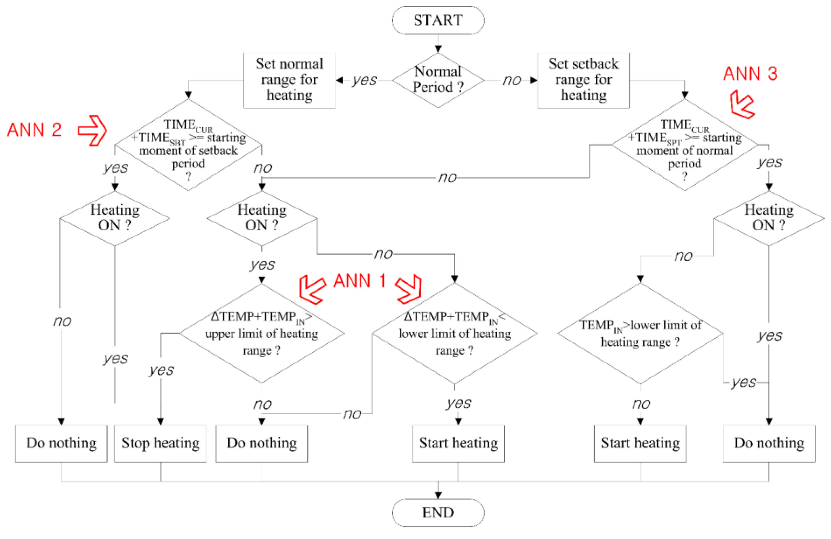
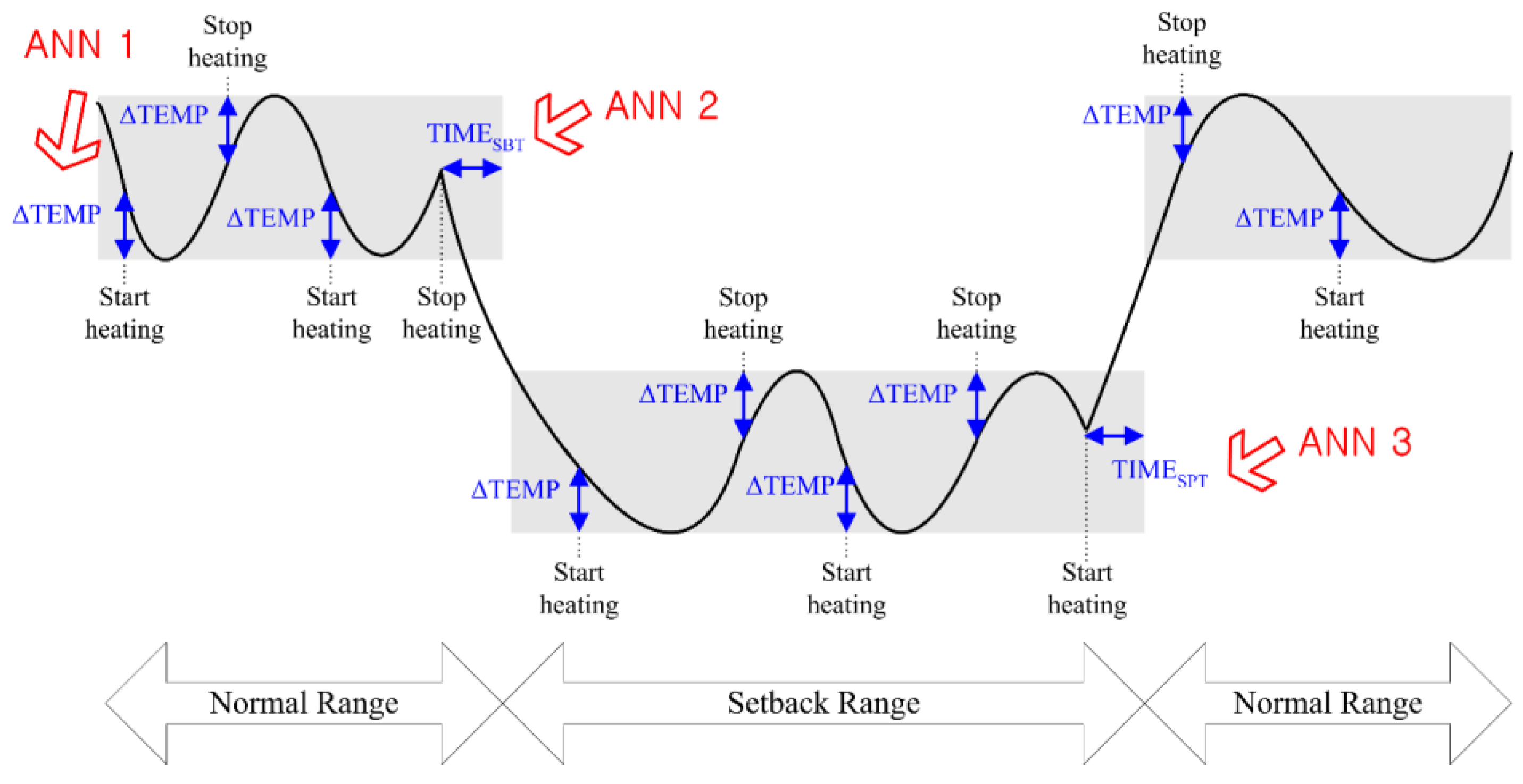
This study develops an ANN prediction model that calculates the required time to raise indoor temperature during the unoccupied setback period to the designated setpoint temperature for the occupied period (TIMESPT). The predicted value from the ANN model is used in the control algorithm to compute the optimal end of the setback period.
For example, if the summation of current time of day (TIMECUR) and predicted time (TIMESPT) during the setback period reaches the start moment of the normal occupied period, then the setback period is predetermined to actually end before the occupied period begins. As a result, the indoor temperature will rise to the comfort level when the occupied period begins. As the prediction model calculates the optimal moment, it can also reduce the energy that will be consumed for pre-heating unnecessarily early before the normal period.
There are two principal reasons to choose the ANN theory to predict TIMESPT in this study. The first is that the ANN model can adopt input variables flexibly. Unlike fuzzy logic (FL) or adaptive neuro fuzzy inference systems (ANFIS), an ANN model can employ a series of inputs for producing outputs. The second reason is that ANN models have proven their stable prediction accuracy and applicability to building thermal controls in the previous studies. These are summarized in Section 2.1. We therefore selected the ANN model over than other machine learning theories.
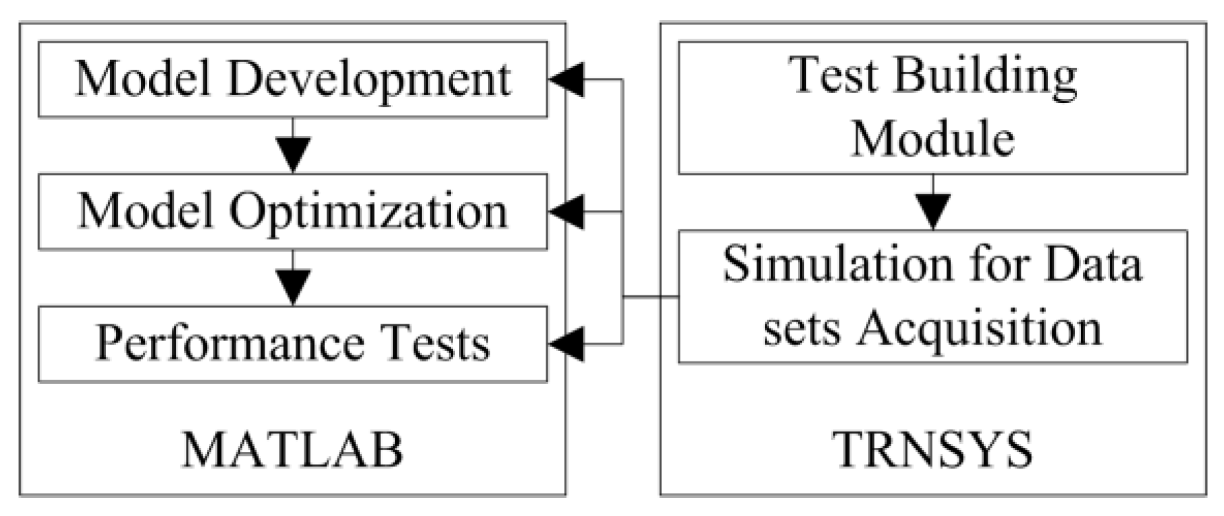
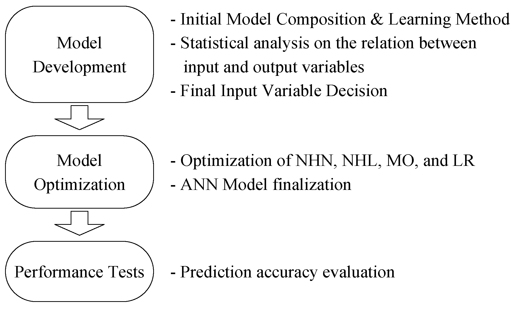
Figure 1 shows the three major steps followed in this study. The first step was model development. The prediction model using ANN was built with initial composition and learning methods. Statistical analysis of the relationship between the input and output variables was performed to find the input variables that have a strong relationship with the output variable. Input variables with a strong relationship were then used as input neurons of the model.
The next step was model optimization. Model parameters such as the number of number of hidden neurons (NHN), hidden layers (NHL), momentum (MO), and learning rate (LR) were optimized to calculate the most accurate output. Optimization was performed in a coupled fashion, so that a series of NHN and NHL were tested together, followed by a series of MO and LR together. The ANN model employed parameter values for which the model predicted the most accurate output.
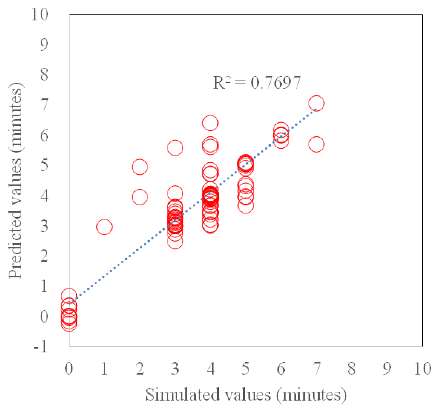
The root mean square error (RMSE) between the predicted results (Pi) and the simulated results (Si) was evaluated for each parameter variation. The Pi values were the predicted results from the ANN model, and the Si values were the calculated results from the test module using the MATLAB and TRNSYS software. The values presenting the least RMSE were assigned to the parameters.
The final step was to conduct performance tests on the optimized model. The prediction accuracy of the ANN model was investigated using new data sets. The applicability of the proposed model was presented based on this performance evaluation.
Two major contributions are provided in this study: (1) a method for designing the ANN model and (2) a specific role for the integrated control algorithm. To overcome the limitations of the previous model, this study conducted two steps (the first and second steps in Figure 1) for finding the meaningful input variables and composing the optimal ANN model. In addition, the proposed model will be embedded in the integrated algorithm. This will be introduced in Section 2.3. Flowchart of the Control Algorithm. Three ANN models will be used to determine comfortable thermal environments while saving energy. In particular, the model developed in this study will provide a comfortable thermal environment at the beginning of the normal occupied period minimizing the unnecessary energy consumption.
The development process is presented in Section 2 including previous studies on the predictive controls using ANN in Section 2.1, the flowchart of the control algorithm in Section 2.2, and the artificial neural network model in Section 2.3. The results of the optimized model are described in Section 3, followed by conclusions in Section 4.

2. Development of the Prediction Model

2.1. Previous Studies on the Predictive Controls Using Artificial Neural Network (ANN)

McCulloch and Pitts suggested a computational model ANN that artificially employs the human neural systems and their learning process [29]. Diverse studies have been conducted for developing ANN models that can predict thermal conditions such as indoor temperature and humidity [30] as well as outdoor temperature [31]. In addition, ANN models were proposed to forecast load and energy for building thermal conditioning [32,33,34,35,36]. The values predicted from the ANN model worked as fundamental determinants for controlling building thermal conditions more comfortably and energy-efficiently.
ANN models present the potential to provide comfortable and energy-efficient thermal environments. Moon et al. [2,37] suggested the use of ANN models to control a variety of thermal targets, such as indoor temperature, humidity, and predicted mean vote (PMV) of a residential building. The predicted future thermal conditions from the ANN model were useful to maintain a more comfortable and stable thermal environment. In addition, a variety of heating and cooling systems were controlled by ANN models, including: the hydronic heating system of solar buildings [38,39], radiant heating system [40,41], evaporative condenser [42], absorption chiller system [43], ground coupled heat pump [44,45,46,47], integrated control of heating or cooling systems and the opening of double skin envelope (DSE) buildings [48,49,50,51,52], photovoltaic module efficiency estimation [53], etc. In addition, the collaborative approach that employed several theories, such as ANN and fuzzy logic, presented successful results to supply thermal comfort [40,54]. These studies demonstrated the superiority of ANN methods over conventional mathematical models, such as proportional-integral-derivative (PID) controllers and regression models. Algorithms employing ANN models accurately predict the thermal loads and proper control of heating and cooling systems resulting in more comfortable thermal environments with energy savings.

2.2. The Artificial Neural Network Model (ANN)

The ANN model in this study focused on calculating the time (TIMPSPT) required for the current indoor temperature during the unoccupied setback period to ascend to the target setpoint temperature of the occupied period. Figure 2 shows the flow of the ANN model development process. The ANN model in this study incorporated Transient Systems Simulation (TRNSYS 16.1) software [55] and Matrix Laboratory (MATLAB) [56] programming software. The test module was modelled using the TRNSYS software where data sets for ANN model training, optimization, and prediction performance tests were collected. After completion of the data collection, the ANN model was developed using MATLAB off-line.
Figure 3 shows the initial model composition suggested in the first step of development. The initial input layer used six input neurons: current indoor air temperature (TEMPIN, °C), variance of indoor air temperature from the preceding control cycle (ΔTEMPIN, °C), current outdoor air temperature (TEMPOUT, °C), variance of outdoor air temperature change from preceding one hour (ΔTEMPOUT, °C), temperature difference from the target setpoint temperature (TEMPDIF, °C), and the amount of solar radiation (SOL, kJ/m2h). Each input value was normalized to between 0 and 1. The actual ranges of each input neuron were 10…30 (TEMPIN), −10…10 (ΔTEMPIN), −20…40 (TEMPOUT), −10…10 (ΔTEMPOUT), 0…10 °C (TEMPDIF), and 0…5000 kJ/m2h (SOL), respectively.
Four hidden neurons were used in each of the three hidden layers based on the findings of a previous study [52], that proposed four hidden neurons and three hidden layers as the optimal composition to predict the future temperature. The hidden neurons used the tangent-sigmoid transfer function to transfer calculation results in the neuron. Each hidden layer repeats the identical process. Lastly, the output layer employs one output neuron TIMESPT, and uses the pure linear transfer function to produce the final output.
One hundred training data sets were prepared for the training model. Each data set was composed of six input values (TEMPIN, ΔTEMPIN, TEMPOUT, ΔTEMPOUT, TEMPDIF, and SOL) and one output value (TIMESPT). The sliding-window method was used to manage the training data sets. Therefore, when a new data set was acquired, the new set replaced the oldest set. Then training was conducted. The Levenberg-Marquardt algorithm was used for the model training with a 0.0-min goal, 1000-times epoch, 0.2-momentum, and 0.6-learning rate, which were found to be the optimal values by a previous study [57].
Figure 4 shows the test module in which the data sets were acquired and Table 1 summarizes the detailed features of the module. The location of the test module was assumed to be in Seoul, South Korea, where winters are cold and dry. Data sets were collected from 1 November to 28 February. Typical meteorological year (TMY2) data was used as weather data. Four data sets were collected per day. For example, the setback temperature was applied at 08:00 a.m. After one hour, the normal setpoint temperature was set at 09:00 a.m. and the six input values were collected at that time. After a certain period (e.g., 30 min), the indoor temperature will reach the normal setpoint temperature. In this case, the output value was 30 min, and one set of data was prepared. After data set acquisition, the set temperature for the heating system is returned to the setback temperature. Then the same process is repeated three times (at 12:00, 15:00, and 18:00) a day. Therefore, 480 data sets were collected, and one hundred sets were randomly selected for initial training.
The dimension of the module was 4.2 m (width), 3.6 m (depth), and 3.05 m (height) approximating the basic and the simplest residential space. The envelope components were assumed to have 3.72, 0.71, 6.80, 3.70 m2·K/W thermal resistance for the wall, windows, roof, and floor, respectively. The thermal resistances of the envelope were greater than required in Korea (2.78, 0.41, 5.00, and 2.32 m2·K/W for each envelope component). A radiant heating system that could supply 12,000 kJ/h of heat. No windows were installed on the east or west walls, and the window-to-wall ratios were 0.20 and 0.10 for the southern and northern walls, respectively. The moderate value for the infiltration rate was assumed to be 2.0 air changes per hour (ACH), which is a normal value. Two occupants, lighting fixtures, and equipment were considered for calculating the internal heat gain.
The model development process continued with a statistical analysis to investigate the relationship between the initial input variables and the output variable. This relationship analysis determined that the input variables that had a strong relevance (R2) to be used as input neurons. One hundred new data sets were used for the analysis.
The second step of the ANN model development was the optimization of the model structure and learning method. The purpose of the optimization was to modify the model to calculate the output more accurately. The structure and the learning method affect the prediction performance and therefore need to be adjusted to produce accurate and stable output [27]. The ANN model structure is determined with a series of input, hidden, and output layers and neurons. The number of input and output layers and neurons were fixed in this study. The optimization factors for this study were the number of hidden neurons (NHN) and hidden layers (NHL).
Learning Rate (LR) and Momentum (MO) are the principal two factors for the ANN model learning method. The LR controls the impact degree of the new data set on the weight changes between neurons when the iterative training is conducted. The LR is related to the degree of adaptation to the new data set as well as the stability of the prediction results. MO considers the trend of the weight changes on the previous training process when the current training is conducted. Proper MO prevents the model from falling into local minima. Since the LR and MO significantly affect the prediction results, these two factors were optimized in this study.
Table 2 summarizes the tested values of each parameter. A coupled fashion was employed for the parametrical optimization. That is, a series of NHN and NHL were tested in combination with each other, then a series of MO and LR were tested in combination. During the optimization process of the first two parameters (i.e., NHN and NHL), the other two parameters (i.e., MO and LR) were fixed as the initial values (0.2 for momentum and 0.6 for learning rate, as suggested in the previous study [54]). Once the optimal values for the first two parameters (NHN and NHL) were found, then the tests for the last two parameters were conducted. During the tests for the last two parameters, the values of the first two parameters were fixed as optimal values found in the previous process. Another 100 data sets were newly collected for the optimization using the identical method to collect data sets for the initial model training and relationship analysis.
After optimization, the third development step tested the prediction accuracy of the optimized ANN model. A further hundred checking data sets were acquired from the identical test module. The statistical correlation (R2) between Pi and Si was analyzed to investigate the prediction accuracy.

2.3. Flowchart of the Control Algorithm

Multiple ANN models including the one developed in this study will be embedded in the control algorithm, which we will develop in further studies. Figure 5 shows the conceptual flowchart of the control algorithm for the heating system. In order to determine the working condition of the heating system, the algorithm uses the period of the day, TIMECUR, TEMPIN, ΔTEMP, TIMESBT, and TIMESPT as determinants. Three ANN models are applied to predict ΔTEMP, TIMESBT, TIMESPT, respectively. Table 3 summarizes their purpose. Two of the ANN models have already been developed, and previous studies introduced their purpose and performance. Those models are ΔTEMP to determine the working mode of the heating system, and TIMESBT to determine the optimal start of the setback period. The last ANN model proposed in this study is applied to determine the optimal end of the setback period based on the predicted TIMESPT.
Figure 6 conceptually shows the temperature profile of the day. By providing the predicted values—ΔTEMP, TIMESBT, and TIMESPT, the three ANN models can help to create more comfortable and stable thermal conditions. In particular, the ANN model (ANN 3) developed in this study predicts the TIMESPT, and this predicted value is used to predetermine the end of setback. By predetermining the end of the setback period, the temperature at the beginning moment of the occupied period is closer to the normal range. For example, if the current indoor temperature is 19.0 °C during the unoccupied setback period and the designated target setpoint temperature is 23.0 °C, the TIMESPT is the amount of minutes needed to raise the current indoor temperature from 19.0 to 23.0 °C. If the sum of TIMPSPT and the current time reaches the beginning moment of the normal setpoint period (i.e., the occupied period), the algorithm determines the normal setpoint temperature to be employed at that moment before the actual occupied period begins.
Figure 7 shows the flow of algorithm operation. As with the ANN model development process, the algorithm development and operation were conducted using TRNSYS and MATLAB. The building and system were modelled using the TRNSYS software. The current indoor and outdoor thermal conditions were collected and transferred to the control algorithm developed using MATLAB. The data was used for the iterative training of the ANN model and for predicting TIMESPT. Based on the TIMESPT, the algorithm decided how to operate the heating system, which would be transferred to the system in the TRNSYS. This process was repeated in a closed loop. Figure 8 shows the modeling results in the TRNSYS, while Table 4 summarizes the types and roles used in the TRNSYS modeling result.

3. Results Analysis

3.1. Selection of Input Neurons

To select the meaningful input neurons for calculating the output neuron, the coefficient of determination (R2) between TEMPIN, ΔTEMPIN, TEMPOUT, ΔTEMPOUT, TEMPDIF, and SOL (input variables) and TIMESPT (output variable) of the initial model were investigated. The results are summarized in Table 5. The coefficient of determination (R2) was calculated for the diverse cases of applying different setback temperatures from 16.5 (setback operating range: 15.0 to 18.0 °C) to 20.5 °C (setback operating range: 19.0 to 22.0 °C).
The R2 between two inputs (TEMPIN and TEMPDIF) and TIMESPT was relatively strong. As the lower setback temperature was applied, the correlation results were higher. When the setback temperature was set to 16.5 °C (the normally recommended setback temperature), the correlation was 0.9330. When the setback temperature was 20.5 °C, it decreased to 0.1435 because the setback temperature was not significantly different from the 21.5 °C setpoint temperature.
Meanwhile, the R2 between other input variables and output variable were unstable and less significant. They ranged from 0.0008 to 0.4768. The input variables with higher R2 were determined as final input neurons of the initial ANN model. Therefore, the new model had two input neurons: TEMPIN and TEMPDIF.

3.2. Model Optimization

Table 6 summarizes the root mean square error (RMSE) results between the Pi and Si for the different combinations of NHN and NHL. The RMSE for a different number of hidden neurons (1 to 10) and hidden layers (1 to 10) presented a wide range of difference. The RMSE for all test cases ranged from 0.74740 min to 1688.48783 min. The case presenting the least RMSE was the model employing 3 NHN and 9 NHL. Therefore, the optimal composition regarding NHN and NHL was determined to be 3 and 9, respectively.
Table 7 summarizes the RMSE results for the different MO (0.1 to 1.0) and LR (0.1 to 1.0). The values for NHN and NHL were fixed as 3 and 9, as found in the previous step. The least RMSE was presented by a model with 0.9 MO and 0.9 LR. For this case, the RMSE was 0.74739 min. Thus, the optimized ANN model employed these values for momentum and learning rate.
Figure 9 shows the ANN model after correlational analysis for the input selection, as well as optimization for the composition and learning method. The final model had two input neurons—TEMPIN and TEMPDIF; 3 NHN; 9 NHL; 0.9 MO; and 0.9 LR.

3.3. Prediction Accuracy

To investigate the accuracy of the prediction results from the optimized ANN model, Pi and Si for the new 100 checking data sets were compared. Figure 10 shows that the results of Pi and Si display a similar pattern. The average difference between them was 0.45 min, which ranged from 0.0 min to 3.9 min. In addition, Figure 11 summarizes the distribution of difference. For 87 of the cases, the difference between Pi and Si was less than 1.0 min. Nine cases were between 1 and 2 min, and four cases were over 2 min.
Figure 12 presents the correlation (R2) between Pi and Si. The Pi and Si show similarity with 0.7697 R2. The time required to raise the indoor temperature to the normal setpoint temperature was not as big as expected. The longest period was 7 min in the simulation in Figure 10. Therefore, a small difference between the simulated and predicted values could cause a significant decrease in R2. When the model is applied to the actual building where longer time is required to raise the temperature to the normal setpoint temperature, R2 is expected to increase. In addition, the CVRMSE (coefficient of variation root mean squared error) between Pi and Si was calculated as 22.74%. According to the ASHRAE Guideline14-Measurement of energy and demand savings [59], the prediction model can prove its prediction accuracy with a CVRMSE value under 30%. Thus, the ANN model in this study proved its prediction accuracy.
The analysis results about the prediction accuracy and correlation between Pi and Si implies that the ANN model can properly predict the ascending time for the pre-determined operation of the heating system during the unoccupied period. Based on the findings, the model presented its potential to be applied in the control algorithm for suggesting the optimal ending moment of the setback temperature for the heating system.

4. Conclusions

In order to develop an ANN prediction model for calculating the time (TIMESPT) required to raise indoor temperature during the unoccupied setback period to the designated target setpoint temperature, three major steps were completed in this study: (1) model development; (2) model optimization; and (3) performance evaluation. Our findings are summarized as follows:
(1)
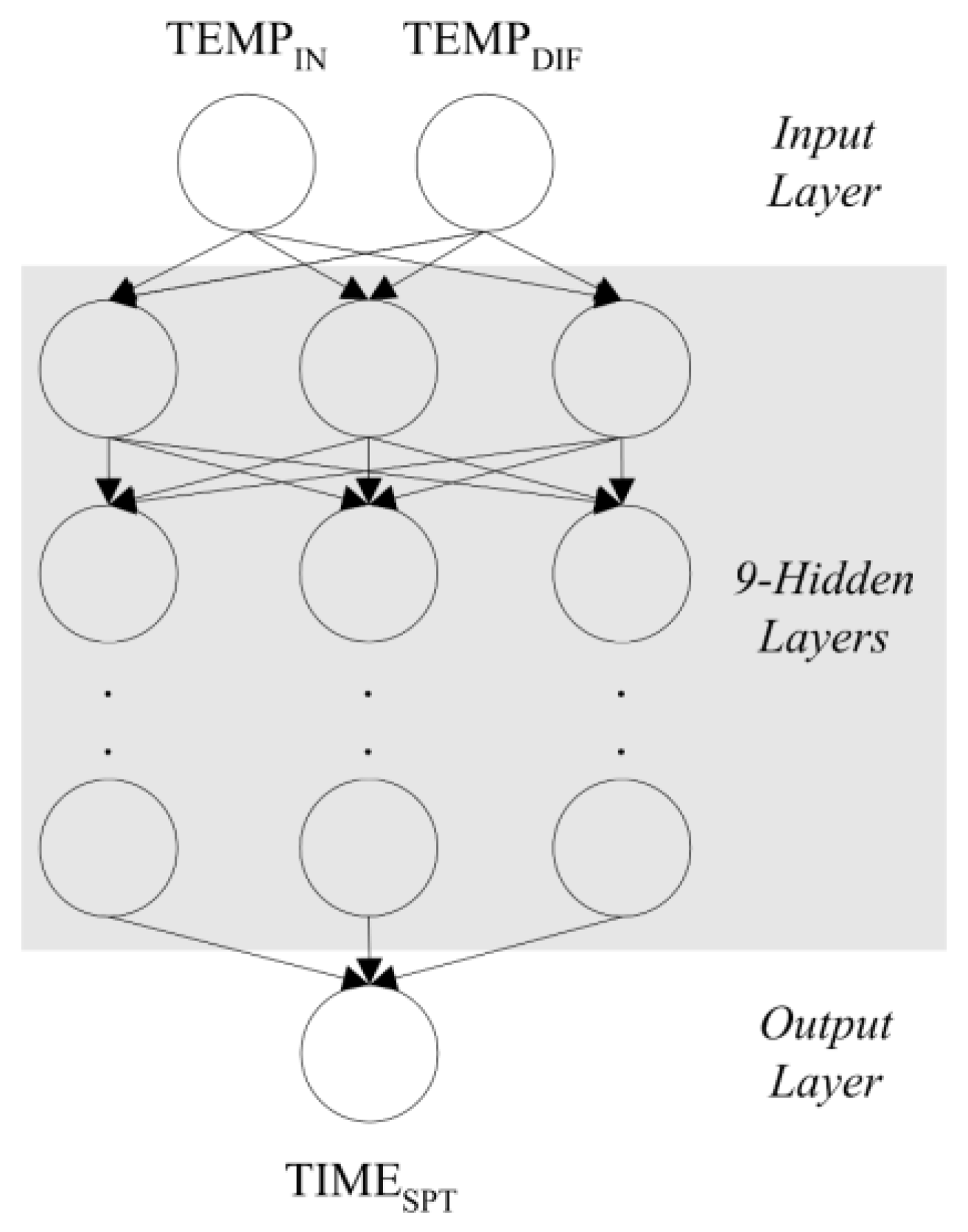
The correlation analysis (R2) between input variables and output variable (1st step) revealed that TEMPIN and TEMPDIF (input variables) presented relatively strong relationships with TIMPSPT (output variable). Therefore, these two variables were selected as input neurons for the initial ANN model.
(2)
Using RMSE to analyze the difference between the simulated outputs (Si) and predicted outputs (Pi) from the ANN model for different ANN parameter values (2nd step) revealed that the least RMSE was produced when applying nine hidden neurons in each hidden layer, three hidden layers, a 0.9 momentum, and a 0.9 learning rate to the ANN model. Therefore, the ANN model was optimized with these final values.
(3)
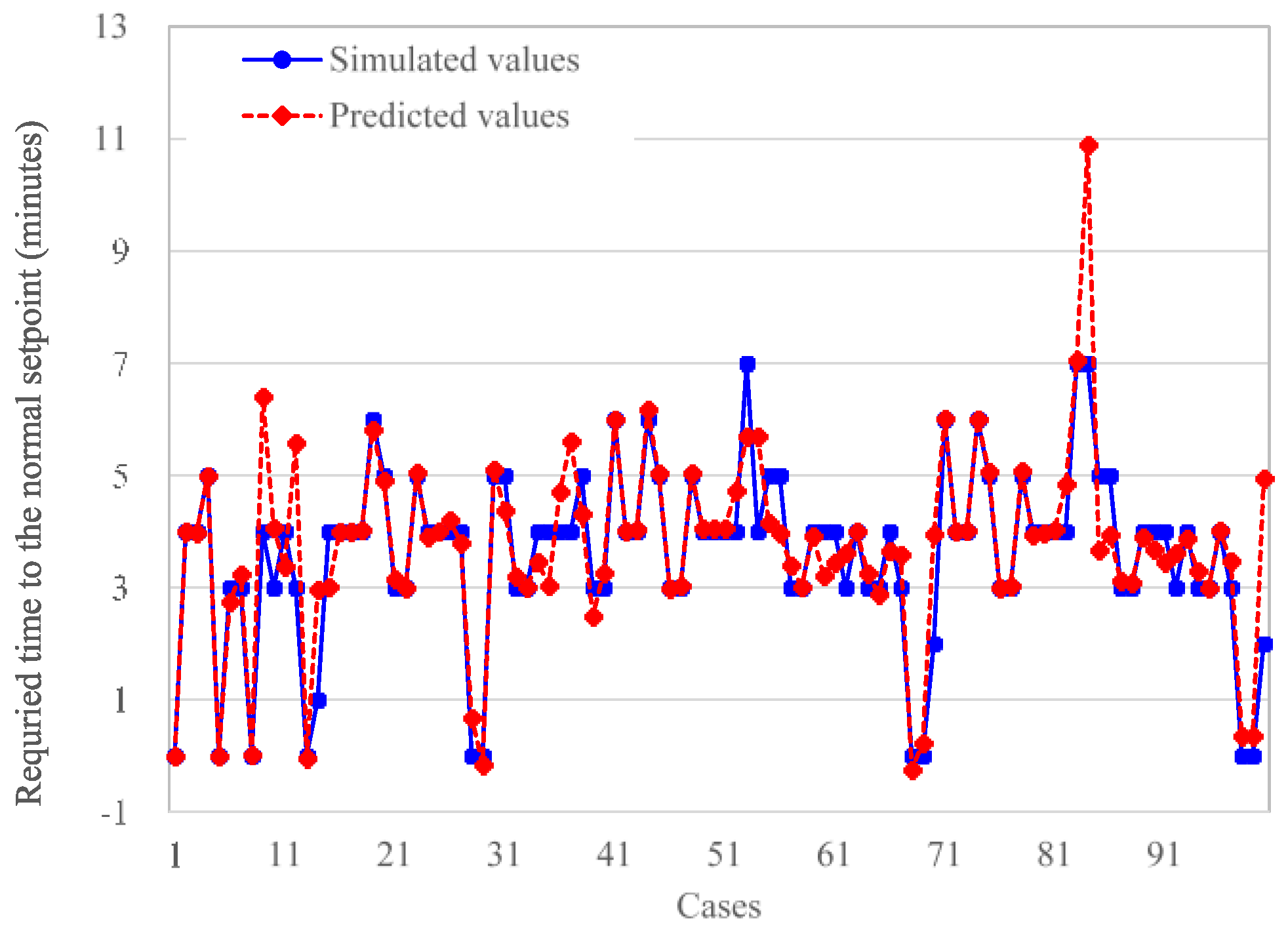
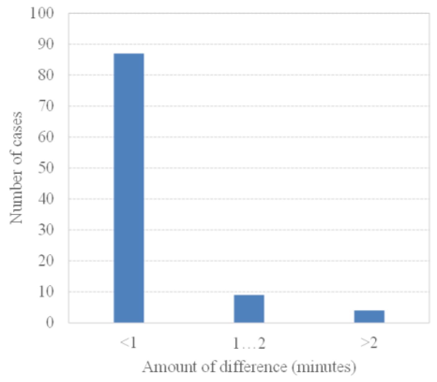
From the performance tests, the proposed ANN model proved its prediction accuracy. The CVRMSE between the simulated outputs and predicted outputs (22.74%) was lower than the generally accepted level (30.0%). In addition, the difference between them for most of the cases was less than 1 min.
In conclusion, based on the previous study [27,28], the more progressive methodology was applied for composing and optimizing the ANN model in this study. First, the meaningful input variables were selected based on their statistical relationship analysis. Then structure and learning methods for the model were optimized in a coupled fashion. The model developed using the new method showed an acceptable prediction accuracy, therefore it was applied to the control algorithm.
The control algorithm employed multiple ANN models. As summarized in Table 1, each model had its prediction target. Using the predicted values from three ANN models, the heating system will start and stop the setback period more accurately as well as create more comfortable and stable indoor temperature conditions.
Overall, we used limited boundary conditions for the performance tests in this study. To ensure that the potential results can be achieved, these performance tests should be conducted in an actual building. Along with the field tests, additional performance tests should be conducted. To provide a solid basis for the proposed method, using other types of simulation methods should also be undertaken. Using MATLAB and EnergyPlus software, and incorporating it with Building Controls Virtual Test Bed (BVCTB) for connecting the two, is proposed as the good method to test the predictive control strategies [60,61].
In addition, the proposed ANN model performance needs to be comparatively investigated by using diverse optimization schemes such as the constructal theory or entropy generation minimization methods. Also, other machine learning methods such as support vector machine (SVM), random neural network (RNN), and model predictive controller (MPC), should be compared to the proposed model. Those methods were stated to predict the indoor temperature conditions more accurately and to maintain indoor temperature more stably in a couple of studies [62,63]. Through these comparative tests, the most applicable method will be found. Finally, the control algorithm, as previously shown in 
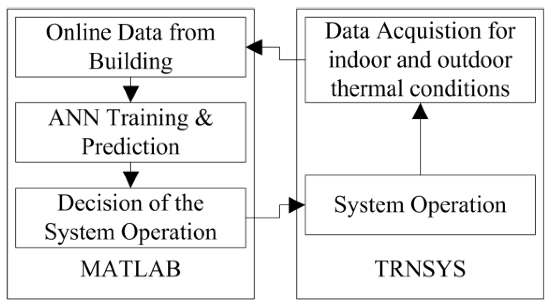
Figure 2, needs to be organized to employ the proposed prediction model and tested for its performance in further studies.

Acknowledgments

This research was supported by the Basic Science Research Program through the National Research Foundation of Korea (NRF) funded by the Ministry of Education, Science and Technology (grant number: 2015R1A1A1A05001142).

Author Contributions

All authors participated in the preparation, research design, method and analysis of this project. All authors discussed and finalized the analysis results to prepare this manuscript.

Conflicts of Interest

The authors declare no conflict of interest.

Nomenclature

TEMPINcurrent indoor air temperature, °C
ΔTEMPINvariance of indoor air temperature from the preceding control cycle, °C
TEMPOUTcurrent outdoor air temperature, °C
ΔTEMPOUTvariance of outdoor air temperature from preceding one hour, °C
TEMPDIFtemperature difference from the target setpoint temperature, °C
SOLthe amount of solar radiation, kJ/m2h
ΔTEMPovershoot or undershoot of indoor air temperature after changing the working mode of the heating system
TIMECURcurrent time of day
TIMPSPTascending time of indoor temperature by heating operation during the setback period to the designated setpoint temperature, minutes
TIMESBTrequired time for descending indoor temperature during the normal period to the designated setback temperature, minutes
NHNnumber of hidden neurons
NHLnumber of hidden layers
MOmomentum
LRlearning rate
PiANN predicted value
Sinumerically simulated value

References

  1. Klepeis, N.E.; Nelson, W.C.; Ott, W.R.; Robinson, J.P.; Tsang, A.M.; Switzer, P.; Behar, J.V.; Hern, S.C.; Engelmann, W.H. The national human activity pattern survey (NHAPS) a resource for assessing exposure to environmental pollutants. J. Expo. Environ. Epidemiol. 2001, 11, 231–251. [Google Scholar] [CrossRef] [PubMed]
  2. Moon, J.W.; Kim, J. ANN-based thermal control models for residential buildings. Build. Environ. 2010, 45, 1612–1625. [Google Scholar] [CrossRef]
  3. Horr, Y.A.; Arif, M.; Kaushik, A.; Mazroei, A.; Katafygiotou, M.; Elsarrag, E. Occupant productivity and officie indoor environment quality: A review of the literature. Build. Environ. 2016, 105, 369–389. [Google Scholar] [CrossRef]
  4. Berglund, B.; Brunekreef, B.; Knöppe, H.; Lindvall, T.; Maroni, M.; Molhave, L.; Skov, P. Effects of indoor air pollution on human health. Indoor Air 1992, 2, 2–25. [Google Scholar] [CrossRef]
  5. Brasche, S.; Bullinger, M.; Morfeld, M.; Gebhardt, H.J.; Bischof, W. Why do women suffer from sick building syndrome more often than men?—Subjective higher sensitivity versus objective causes. Indoor Air 2001, 11, 217–222. [Google Scholar] [CrossRef] [PubMed]
  6. Fisher, P.H.; Kriz, B.; Martuzzi, M.; Wojtuniak, B.; Lebret, E.; Reeuwijk, H.V.; Pikhart, H.; Briggs, D.; Gorynski, P.; Elliott, P. Risk factors indoors and prevalences of childhood respiratory health in four countries in western and central Europe. Indoor Air 1998, 8, 244–254. [Google Scholar] [CrossRef]
  7. Garrett, M.H.; Abramson, M.J.; Hooper, B.M.; Rayment, P.R.; Strasser, R.P.; Hooper, M.A. Indoor environmental risk factors for respiratory health in children. Indoor Air 1998, 8, 236–243. [Google Scholar] [CrossRef]
  8. Stenerg, B.; Mild, K.H.; Sandström, M.; Sundell, J.; Wall, S. A prevalence study of the sick building syndrome (SBS) and facial skin symptoms in office workers. Indoor Air 1993, 3, 71–82. [Google Scholar] [CrossRef]
  9. Ministry of Knowledge Economy. A Law for Rationalization of Energy Consumption. Ministry of Knowledge Economy. Available online: http://www.mke.go.kr (accessed on 19 June 2013).
  10. Moon, J.W.; Han, S. Thermostat strategies impact on energy consumption in residential buildings. Energy Build. 2011, 43, 338–346. [Google Scholar] [CrossRef]
  11. Karjalainen, S. Thermal comfort and use of thermostats in Finnish homes and offices. Build. Environ. 2009, 44, 1237–1245. [Google Scholar] [CrossRef]
  12. Chung, C.Y.; Kim, H.J.; Bae, N.R. Research on thermal environment in apartments’ living rooms and residents’ control behaviors of a thermostat. J. Archit. Inst. Korea 2005, 21, 209–216. [Google Scholar]
  13. Humphreys, M.; Nicol, F. Understanding the adaptive approach to thermal comfort. ASHRAE Trans. 1998, 104, 991–1004. [Google Scholar]
  14. Manning, M.M.; Swinton, M.C.; Szadkowski, F.; Gusdorf, J.; Ruest, K. The effect of thermostat set-back and set-up on seasonal energy consumption, surface temperatures and recovery times at the CCHT Twin House Facility. ASHRAE Trans. 2007, 13, 1–12. [Google Scholar]
  15. Ingersoll, J.; Huang, J. Heating energy use management in residential buildings by temperature control. Energy Build. 1985, 1, 27–35. [Google Scholar] [CrossRef]
  16. Beckey, T.; Nelson, L.W. Field test of energy savings with thermostat setback. ASHRAE J. 1981, 1, 67–70. [Google Scholar]
  17. Nelson, L.W.; MacArthur, J.W. Energy savings through thermostat set-back. ASHRAE Trans. 1978, 82, 319–334. [Google Scholar]
  18. Nelson, L.W. Reducing fuel consumption with night setback. ASHRAE J. 1973, 8, 41–49. [Google Scholar]
  19. Rosenfeld, A.H. Notes on residential fuel use: Thermostat and window management. Energy Build. 1977, 1, 99–101. [Google Scholar] [CrossRef]
  20. Guo, W.; Nutter, D.W. Setback and setup temperature analysis for a classic double-corridor classroom building. Energy Build. 2010, 42, 189–197. [Google Scholar] [CrossRef]
  21. Programmable Thermostats as Means of Generating Energy Savings: Some Pros and Cons. Available online: https://sites.ualberta.ca/~cbeedac/publications/documents/progtherm1_000.pdf (accessed on 7 October 2016).
  22. Maheshwari, G.P.; Al-Taqi, H.; Al-Murad, R.; Suri, R.K. Programmable thermostat for energy saving. Energy Build. 2001, 33, 667–672. [Google Scholar] [CrossRef]
  23. Keshtkar, A.; Arzanpour, S.; Keshtkar, F. Adaptive residential demande-side management using rule-based techniques in smart grid environments. Energy Build. 2016, 133, 281–294. [Google Scholar] [CrossRef]
  24. Chassin, D.P.; Stoustrup, J.; Agathoklis, P.; Djilali, N. A new thermostat for real-time price demand response: Cost, comfort and energy impacts of discrete-time control without deadband. Appl. Energy 2015, 155, 816–825. [Google Scholar] [CrossRef]
  25. Alhashme, M.; Ashgriz, N. A virtual thermostat for local temperature control. Energy Build. 2016, 126, 323–339. [Google Scholar] [CrossRef]
  26. Pritoni, M.; Woodley, J.M.; Modera, M.P. Do occupancy-responsive learning thermostats save energy? A field study in university residence halls. Energy Build. 2016, 127, 469–478. [Google Scholar] [CrossRef]
  27. Yang, I.; Kim, K. Prediction of the time of room air temperature descending for heating systems in buildings. Build. Environ. 2004, 39, 19–29. [Google Scholar] [CrossRef]
  28. Lee, J.Y.; Yang, I.H.; Song, S.Y.; Kim, H.S.; Kim, K.W. A study of the predictive control of the ondol system in apartments. In Proceedings of the Sixth International Building Performance Simulation Association, Kyoto, Japan, 13–15 September 1999.
  29. McCulloch, W.; Pitts, W.A. Logical calculus of ideas immanent in nervous activity. Bull. Math. Biophys. 1943, 5, 115–133. [Google Scholar] [CrossRef]
  30. Mba, L.; Meukam, P.; Kemajou, A. Application of artificial neural network for predicting hourly indoor air temperature and relative humidity in modern building in humid region. Energy Build. 2016, 121, 32–42. [Google Scholar] [CrossRef]
  31. Papantoniou, S.; Kolokotsa, D. Prediction of outdoor air temperature using neural networks: Application in 4 European cities. Energy Build. 2016, 114, 72–79. [Google Scholar] [CrossRef]
  32. Deb, C.; Eang, L.S.; Yang, J.; Santamouris, M. Forecasting diurnal cooling energy load for institutional buildings using Artificial Neural Networks. Energy Build. 2016, 121, 284–297. [Google Scholar] [CrossRef]
  33. Chae, Y.T.; Horesh, R.; Hwang, Y.; Lee, Y.M. Artificial neural network model for forecasting sub-hourly electricity usage in commercial buildings. Energy Build. 2016, 111, 184–194. [Google Scholar] [CrossRef]
  34. Li, K.; Hu, C.; Liu, G.; Xue, W. Building’s electricity consumption prediction using optimized artificial neural networks and principal component analysis. Energy Build. 2015, 108, 106–113. [Google Scholar] [CrossRef]
  35. Paudel, S.; Elmtiri, M.; Kling, W.L.; Corre, O.L. Pseudo dynamic transitional modeling of building heating energy demand using artificial neural network. Energy Build. 2015, 70, 81–93. [Google Scholar] [CrossRef] [Green Version]
  36. Escrivá-Escrivá, G.; Álvarez-Bel, C.; Roldán-Blay, C.; Alcázar-Ortega, M. New artificial neural network prediction method for electrical consumption forecasting based on building end-uses. Energy Build. 2011, 43, 3112–3119. [Google Scholar] [CrossRef]
  37. Moon, J.W. Performance of ANN-based predictive and adaptive thermal control methods for disturbances in and around residential buildings. Build. Environ. 2011, 48, 15–26. [Google Scholar] [CrossRef]
  38. Argiriou, A.A.; Bellas-Velidis, I.; Kummert, M.; Andre, P. A neural network controller for hydronic heating systems of solar buildings. Neural Netw. 2004, 17, 424–440. [Google Scholar] [CrossRef] [PubMed]
  39. Argiriou, A.A.; Bellas-Velidis, I.; Balaras, C.A. Development of a neural network heating controller for solar buildings. Neural Netw. 2000, 13, 811–820. [Google Scholar] [CrossRef]
  40. Morel, N.; Bauer, M.; El-Khoury, M.; Krauss, J. Neurobat, a predictive and adaptive heating control system using artificial neural networks. Int. J. Sol. Energy 2001, 21, 161–201. [Google Scholar] [CrossRef]
  41. Lee, J.Y.; Yeo, M.S.; Kim, K.W. Predictive control of the radiant floor heating system in apartment buildings. J. Asian Archit. Build. Eng. 2002, 1, 105–112. [Google Scholar] [CrossRef]
  42. Abbassi, A.; Bahar, L. Application of neural network for the modeling and control of evaporative condenser cooling load. Appl. Therm. Eng. 2005, 25, 3176–3186. [Google Scholar] [CrossRef]
  43. Chow, T.T.; Lin, Z.; Song, C.L.; Zhang, G.Q. Applying neural network and genetic algorithm in chiller system optimization. In Proceedings of the Seventh International Building Performance Simulation Association, Rio de Janeiro, Brazil, 13–15 August 2001.
  44. Hikmet, E.; Mustafa, I.; Abdulkadir, S.; Mehmet, E. Forecasting of a ground-coupled heat pump performance using neural networks with statistical data weighting pre-processing. Int. J. Therm. Sci. 2008, 47, 431–441. [Google Scholar]
  45. Hikmet, E.; Mustafa, I.; Abdulkadir, S.; Mehmet, E. Artificial neural networks and adaptive neuro-fuzzy assessments for ground-coupled heat pump system. Energy Build. 2008, 40, 1074–1083. [Google Scholar]
  46. Hikmet, E.; Mustafa, I.; Abdulkadir, S.; Mehmet, E. Performance prediction of a ground-coupled heat pump system using artificial neural networks. Expert Syst. Appl. 2008, 35, 1940–1948. [Google Scholar]
  47. Fannou, J.C.; Rousseau, C.; Lamarche, L.; Kajl, S. Modeling of a direct expansion geothermal heat pump using artificial neural networks. Energy Build. 2014, 81, 381–390. [Google Scholar] [CrossRef]
  48. Moon, J.W.; Lee, J.; Chang, J.D.; Kim, S. Preliminary performance tests on artificial neural network models for opening strategies of double skin envelopes in winter. Energy Build. 2014, 75, 301–311. [Google Scholar] [CrossRef]
  49. Kim, S.; Lee, J.; Moon, J.W. Performance evaluation of artificial neural network-based variable control logic for double skin enveloped buildings during the heating season. Build. Environ. 2014, 82, 328–338. [Google Scholar] [CrossRef]
  50. Moon, J.W.; Lee, J.; Kim, S. Application of control logic for optimum indoor thermal environment in buildings with double skin envelope systems. Energy Build. 2014, 85, 59–71. [Google Scholar] [CrossRef]
  51. Moon, J.W. Integrated control of the cooling system and surface openings using the artificial neural networks. Appl. Therm. Eng. 2015, 78, 150–161. [Google Scholar] [CrossRef]
  52. Baik, Y.K.; Moon, J.W. Development and performance evaluation of optimal control logics for the two-position- and variable-heating systems in double skin façade buildings. Int. J. Korea Inst. Ecol. Archit. Environ. 2014, 14, 71–77. [Google Scholar] [CrossRef]
  53. Ceylan, İ.; Gedik, E.; Erkaymaz, O.; Gürel, A.E. The artificial neural network model to estimate the photovoltaic module efficiency for all regions of the Turkey. Energy Build. 2014, 84, 258–267. [Google Scholar] [CrossRef]
  54. Collotta, M.; Messineo, A.; Nicolosi, G.; Pau, G. A dynamic fuzzy controller to meet thermal comfort by using neural network forecasted parameters as the input. Energies 2014, 7, 4727–4756. [Google Scholar] [CrossRef]
  55. University of Wisconsin. TRNSYS16.1. Available online: http://www.sel.me.wisc.edu/trnsys/ (accessed on 13 October 2015).
  56. MathWorks. MATLAB 14, Volume 26. Available online: http://www.mathworks.com; (accessed on 15 October 2015).
  57. Moon, J.W.; Kim, K.; Min, H. ANN-based prediction and optimization of cooling system in hotel rooms. Energies 2015, 8, 10775–10795. [Google Scholar] [CrossRef]
  58. Moon, J.W.; Jung, S.K. Algorithm for optimal application of the setback moment in the heating season using an Artificial Neural Network model. Energy Build. 2016, 127, 859–869. [Google Scholar] [CrossRef]
  59. American Society of Heating, Refrigerating, and Air-Conditioning Engineers, Inc. ASHRAE Guideline14-Measurement of Energy and Demand Savings; ASHRAE: Atlanta, GA, USA, 2002. [Google Scholar]
  60. Prívara, S.; Váňa, Z.; Gyalistras, D.; Cigler, J.; Sagerschinig, C.; Morari, M.; Ferkl, L. Modeling and identification of a large multi-zone office building. In Proceedings of the IEEE International Conference on Control Applications, Denver, CO, USA, 28–30 September 2011.
  61. Li, X.; Wen, J. Building energy consumption on-line forecasting using physics based system identification. Energy Build. 2014, 84, 1–12. [Google Scholar] [CrossRef]
  62. Cai, Q.; Wang, W.; Wang, S. Application of indoor temperature prediction based on SVM and BPNN. In Proceedings of the 27th Chinese Control and Decision, Qingdao, China, 23–25 May 2015.
  63. Javed, A.; Larijani, H.; Ahmadinia, A.; Emmanuel, R. Comparison of the robustness of RNN, MPC, and ANN controller for residential heating system. In Proceedings of the IEEE Fourth International Conference on Big Data and Cloud Computing, Sydney, Australia, 3–5 December 2014.
Figure 1. Development process.
Energies 09 01090 g001
Figure 2. Flow of the artificial neural network (ANN) model development.
Energies 09 01090 g002
Figure 3. The initial ANN model.
Energies 09 01090 g003
Figure 4. Test module for collecting datasets of the ANN model (in meters).
Energies 09 01090 g004
Figure 5. The control algorithm.
Energies 09 01090 g005
Figure 6. A conceptual temperature profile with the predictive control algorithm.
Energies 09 01090 g006
Figure 7. Flow of algorithm operation.
Energies 09 01090 g007
Figure 8. Components for modeling the test module and for data acquisition.
Energies 09 01090 g008
Figure 9. The optimized ANN model.
Energies 09 01090 g009
Figure 10. Comparison of the simulated and predicted times.
Energies 09 01090 g010
Figure 11. Number of cases according to the amount of difference.
Energies 09 01090 g011
Figure 12. Statistical relationship (R2) between the simulated values (Si) and the predicted values (Pi).
Energies 09 01090 g012
Table 1. Features of the test building.
ComponentsFeatures
Location & weather data• Seoul, South Korea (latitude: 37.56° N, longitude: 126.98° E)
• TMY2 data
Dimensions (width × depth × height)4.2 m × 3.6 m × 3.05 m
Envelope insulation (m2·K/W)Exterior walls3.72
Roof6.80
Floor3.70
Windows0.71 with 6 mm gray glass + 16 mm argon gas + 6 mm gray glass
Heating systemRadiant heating: 12,000 kJ/h heat supply
Window to wall ratioEast0.00
West0.00
South0.20
North0.10
Infiltration rate2.0 ACH
Internal gainOccupants2 seated persons performing light work
Lighting5 W/m2
Equipment2 computers with a printer
Table 2. Parametrically tested values of each ANN component.
ComponentsParametrical Values
1st step of the optimizationNHN1, 2, 3, 4, 5, 6, 7, 8, 9, 10
NHL1, 2, 3, 4, 5, 6, 7, 8, 9, 10
2nd step of the optimizationMO0.1, 0.2, 0.3, 0.4, 0.5, 0.6, 0.7, 0.8, 0.9, 1.0
LR0.1, 0.2, 0.3, 0.4, 0.5, 0.6, 0.7, 0.8, 0.9, 1.0
Table 3. ANN models applied in the control algorithm.
TypePurposeNote
ANN 1Predict overshoot or undershoot (ΔTEMP)Developed in a previous study [58]
ANN 2Predict time to the setback temperature (TIMESBT)Developed in a previous study [57]
ANN 3Predict time to the normal setpoint temperature (TIMESPT)Proposed in this study
Table 4. Modeling result and TRNSYS types and roles employed.
TypesRoles
Type9c• Importing a TMY2 weather file for the site
Type16a• Calculating solar radiation on building surfaces
Type33e• Calculating dew-point temperature of surrounding exterior
Type69b• Calculating sky temperature
Type56a-TRNFlow• Calling building modeling result of TRNBUILD
• Calculating indoor temperature of the test building
Type155• Calling the algorithm in MATLAB
• Producing training and checking data sets
• Calculating signal for the cooling system operation
Type65d-2• Producing and displaying the output file
Table 5. Statistical correlation (R2) between input and output variables of the ANN model.
Setback TemperatureTEMPINΔTEMPINTEMPOUTΔTEMPOUTTEMPDIFSOLAR
16.50.93300.09450.47680.06200.93300.0659
17.50.83180.05070.35460.08170.83180.1046
18.50.83820.07060.22840.11620.83820.0847
19.50.52790.25300.00450.00330.52790.0040
20.50.14350.41960.00080.00600.14350.0821
Table 6. RMSE between the simulated and predicted values for various NHN and NHL.
NHN
12345678910
NHL10.9908 2.2508 0.8708 0.8906 0.7876 411.4124 1667.3525 1688.4878 369.0404 390.1868
21.0057 2.1664 1.6023 2.1504 5.5277 1.8164 17.8210 14.1733 6.3433 6.0548
30.7476 0.8494 1.7313 4.5223 6.9102 3.2818 5.6517 1.9963 5.4272 2.3711
40.7533 0.7475 2.6425 6.9115 1.4996 1.5233 2.8315 2.1139 1.5545 1.9412
50.7476 6.7753 1.3164 0.7474 2.0560 1.1627 2.7472 2.0695 1.2443 0.9671
60.7476 0.7533 3.3833 1.6075 1.8473 1.2653 1.8547 1.0211 1.0877 1.3138
70.7533 4.8343 1.8222 2.1438 2.0031 1.0440 1.0838 1.0505 0.9834 0.8582
80.7533 2.6292 0.7533 1.1415 1.2874 1.1312 1.7813 1.0001 0.8808 0.9931
90.7533 0.7475 0.7474 0.7533 1.4850 1.5028 1.0399 1.5618 0.9067 1.8986
100.7533 0.7475 0.9176 1.4497 1.0873 1.3791 1.1780 1.0083 0.8094 0.9838
Table 7. RMSE between the simulated and predicted values for various numbers of MO and LR.
MO
0.10.20.30.40.50.60.70.80.91.0
LR0.10.9809 0.8242 1.7961 1.4502 0.9985 0.7533 1.1771 1.5723 1.2746 1.2490
0.20.7474 0.9572 1.8231 0.8073 1.6544 1.5590 0.7533 2.6946 0.7533 2.2565
0.30.7533 1.4030 1.7982 0.7533 1.0909 1.5723 1.2746 1.2490 0.7474 0.9572
0.41.8231 0.8073 1.6544 1.5590 0.7533 2.6946 0.7533 2.2565 0.7533 1.4030
0.51.7982 1.3875 0.7533 1.4586 1.1192 0.7475 1.6204 1.3738 1.1081 1.2201
0.60.7533 2.3198 1.9942 1.1889 0.7533 1.0230 2.0540 1.6884 0.7533 2.0263
0.73.6128 1.1414 2.1606 1.9982 1.0870 1.1360 1.4460 1.6798 1.4096 1.6103
0.81.3603 1.5333 5.4342 1.0667 1.9131 2.4616 1.4424 0.8519 5.9723 1.0491
0.91.4500 2.1613 0.8646 1.9460 1.1701 1.6084 3.2015 2.2299 0.7474 0.7474
1.00.7533 2.1820 1.0892 1.4702 0.9278 3.1597 0.7533 0.7533 0.9766 1.9512

