
On the Reliability of Optimization Results for Trigeneration Systems in Buildings, in the Presence of Price Uncertainties and Erroneous Load Estimation

Abstract
:
1. Introduction
- -
- A scarce to moderate characterization of the intrinsic features of the stochastic parameters. The probabilistic distribution of energy loads is rarely examined in detail and, in general, trends are studied for a single or very few (up to three, one per climatic season) standard days. This approach has been proven error-prone, since a sufficient number of “standard days” must be selected to achieve optimization results consistent with those that would be obtained adopting a whole set of hourly data for a year [27,28].
- -
- A major focus posed on the mathematical problem, rather than on the actual energetic behaviour of the building and the plant to be installed. This is also proven by the dozens of articles (not discussed in the above literature overview for the sake of brevity) with similar titles but published by “operational research” experts.
- the shape of the daily energy load profiles;
- the relative weights between heating/electric and cooling/electric loads, respectively in winter and in summer;
- the shape of the daily electricity price profiles;
- the relative price of electricity and fuel.
2. Fundamental Features of the Deterministic CHCP Optimization Tool
- Single-Building Optimization (SBO) routine, which optimizes the synthesis, design and operation of a CHCP plant (equipped with thermal energy storage) serving a specific building;
- Multi-Buildings Optimization (MBO) routine, which optimizes the synthesis, design and operation of an integrated trigeneration plant that includes a number of CHP units serving a cluster of buildings via an electric μgrid and a warm water distribution network.
2.1. Variables and Objective Function
- −
- At synthesis level, a number of binary [0, 1] variables, indicated as δcomp, whose values “1” and “0” indicate the options to include or not the related component in the optimal plant lay-out;
- −
- At design level, the electric rated capacity of the CHP unit ( in kWe), the cooling capacity of absorption chiller ( in kWc) and the volume of the heat storage tank (VTES in m3) to be installed;
- −
- At operation level, the rated output (i.e., the load level) of each component at any time step (1 h) is optimized. For the heat storage tank, a hourly average charging/discharging rate is assumed as “operation variable”.
- ○
- The total investment cost, Itot: appropriate linear cost functions are included in a library, developed on the basis of large databases of CHCP components created within previous research activities [31]), so as to express Itot as a function of components’ capacities (i.e., decision variables at design level);
- ○
- The total cost of the fuel consumed over the plant life cycle (assumed to be 15 years), FUELtot, calculated by using annual fuel expenses and summating their values at the “present time” by adopting an appropriate Present Worth Factor (PWF). Of course, FUELtot includes the cost for the fuel consumed by both the CHP unit and the auxiliary boiler(s);
- ○
- The total cost/revenue for the bi-directional power exchange with the grid, Ce.exch, again cumulated and actualized by using the appropriate. No revenues from heat/cooling production are explicitly taken into account, because the CHCP system is assumed not to be connected to any external district heating/cooling network and it cannot consequently sell thermal or cooling energy to external users. However, the “cogenerated” heat and cooling energy obviously contributes to increase the NPV since (i) the recovered heat induces an avoided cost in terms of fuel to the heat-only boiler; and (ii) the cooling production by the absorption chiller induces an avoided electricity consumption in the auxiliary vapor compression chiller;
- ○
- The total maintenance cost, accounted for by assuming an average 0.015 € cost per kWh electricity produced; this value is a reasonable figure for natural gas engines [32].
2.2. Physical Constraints
- −
- Coverage of energy loads: the sum of energy outputs from the different components must be always sufficient to ensure full coverage of energy requests from the building. For instance, the coverage of direct/indirect heat requests is imposed by:where i indicates the time step, H is the thermal output from the prime mover (in kW) in the time step, C is the cooling output by the absorption chiller (that divided by COP gives the heat rate needed to feed this component, thus representing an additional heat load), represents the charging/discharging rate (respectively when negative/positive) during the ith and Dh indicates the heat load. The constraint is imposed as an inequality, in order to allow the algorithm to explore possible solutions where the CHP unit is not strictly operated according to a FTL strategy, and hence some surplus heat can be discarded to the radiator or by exhausting the hot gases. Similar equations are imposed for the coverage of cooling loads (in equality terms, since production of surplus cooling energy is in no case profitable) and for the electrical balance with the grid;
- −
- Production limits: at each time-step, this trivial constraint imposes the production rate of each component not to exceed its rated capacity. For instance, as concerns the CHP unit, we have:where PHRCHP represents the Power to Heat Ratio of the CHP unit. Again, similar equations are imposed for the absorption chiller and the heat storage;
- −
- Heat storage balance: it imposes a relation between the sensible energy stored (STOR) at the beginning of a generic time step “i” and the amount stored at the successive time step “i + 1”:In Equation (3) ∆H% represents an hourly heat loss rate (which depends on the thermal insulation of the tank).
- −
- Congruence between operation and synthesis variables: since each component can be either included or not in the lay-out (depending on the optimal value assumed by the binary 0–1 synthesis variable δcomp), for the CHP unit the following constraint is imposed:This constraint forces the production rate of the CHP unit to zero (for the examined ith time-step) whenever the component is not included in the lay-out (i.e., δcog = 0), while it is not a binding constraint when the CHP unit is included (i.e., δcog = 1), provided that the constant κ is assigned with a conveniently high value (in the order of 105 when Hcog is expressed in kW). Similar constraints are imposed for the absorption chiller and the heat storage tank;
- −
- A number of additional constraints are imposed and not presented here in details for the sake of brevity. Just to provide some brief notes, a first additional condition is related with the technically feasible dynamic operation of the CHP unit: two distinct maximum feasible hourly load variations are imposed, for the ramp-up and ramp-down periods. Such a constraint is imposed to avoid convergence toward solutions that require frequent start-ups and switch-offs of the unit. A second additional (and optional) condition is related with the fulfilment of the eligibility conditions to have the optimized CHCP configuration assessed as “high efficiency cogeneration”, according to the current legislative framework in Europe [33].
3. The Case Study: Base Case and Alternative Scenarios for the Uncertain Data
- -
- All the historical data related with energy consumption had been collected. They essentially consisted of electricity and natural gas consumption derived from the bills; as concerns electricity, also disaggregated consumption data per tariff band (peak, medium-load and off-peak hours) were available;
- -
- Based on interviews with the hotel management and with the technicians and on comparisons with trends available in literature, typical daily profiles for working and non-working days were developed. These profiles were used to spread the historical consumption data and thus obtain the required 8760-values arrays needed as inputs for the optimization tool.
- -
- In large buildings where complex activities take place, any attempt to use more sophisticate approaches (for instance, dynamic simulators of the buildings’ energy performance) would not necessarily provide more reliable load profiles, due to the enormous amounts of hardly predictable data to be collected;
- -
- It is very common, in the energy auditing phase, to base part of the assumptions on the direct contribution provided by the personnel involved in plant operation.
- -
- Completely relied upon the energy load input data that were indicated as “base case”, by the interviews-based energy audit;
- -
- Adopted the current (i.e., at the moment when the feasibility study is assumed to be conducted, year 2005) electricity prices and natural gas price.
3.1. Alternative Scenarios Descending from an Erroneous Load Estimation
- −
- “daily profiles’ shape errors”, consisting in an erroneous assumption of the shape of the daily energy load profiles;
- −
- “heating/electricity and cooling/electricity load ratios estimation errors”, consisting in an erroneous estimation of the fraction of electricity consumption that has been used to supply HVAC systems for space heating and cooling.
3.1.1. Daily Energy Load Profiles’ Shape Errors
- -
- Correct in terms of total daily loads. This assumption is reasonable, since the simple procedure of dividing the monthly consumption of natural gas or electricity by the number of days of the month (eventually introducing some minor corrections to distinguish between working and non-working days) has not relevant margins of errors;
- -
- Erroneous in terms of hourly loads.
- As concerns the space heating load (limited to the winter period), it is assumed that a peak request occurs in the early morning hours (6.00–7.00 a.m., see Figure 1a). This is quite typical for the space heating of large rooms or open spaces (like the Conference rooms or the hall of hotels) or, for smaller rooms, when the plant have been switched off during night-time;
- As concerns the DHW requests, an even higher peak can be expected in the early morning, due to the reasonably high simultaneity factor in the sanitary uses of hot water. Let us observe the adopted modified profile significantly differs from the “base case”, which appears quite unrealistic;
- The “base case” daily cooling load profile, which also was very “flat”, was modified to follow a more common trend for civil applications, with significant increases in the cooling requests after 12.00 a.m. and peak loads occurring in the early afternoon;
- As concerns the electric loads, that should be here intended as electricity uses for equipment and appliances (i.e., excluding any electric consumption for Heating, Ventilation and Air Conditioning units, HVACs), just minor changes are imposed, based on shifting part of the night-time consumption to the day-time hours. This assumption reflects a possible realistic condition, in case the plant owner/manager had overestimated the energy requests for internal and external lighting during night-time.
3.1.2. Heating/Electricity and Cooling/Electricity Load Ratios Estimation
- -
- a base electric load is estimated as average monthly electric consumption in the “intermediate season” (i.e., in the period where neither space heating nor cooling is requested);
- -
- in the summer and winter periods, such a base electric load is subtracted from the actual electricity consumption derived from the supplier’s bills. This procedure, that implicitly relies upon the quasi-constancy of monthly electricity consumption for lighting and appliances throughout the year, allows to get a rough estimation of the additional electric consumption by the heat pump or the chiller;
- -
- The electric consumption for “indirect uses” is finally used to calculate the space heating and cooling loads, by assuming an appropriate Seasonal Coefficient of Performance (SCOP) or Energy Efficiency Ratio (SEER).
- Decreased fraction of electricity consumption for space heating: this modified scenario is based on the assumption that, when deriving the space heating loads following the aforementioned approach, these loads are overestimated by 30%. The resulting modified load profile is shown in Figure 2a, where the load profiles referring to the “base case” are also shown to allow for an easier comparison. In particular, in the figure the curve enveloping the daily peaks of total heat (space heating and DHW) and electric loads are presented. We may observe that the base case and the modified scenario only differ in the winter period (i.e., when space heating is required), and that the modified heat load profile achieves much lower annual peaks (approximately 2200 kW, instead of 3150 kW that is the peak in the base case). A slightly higher electric load consequently results in the winter period, due to the modified shares of actual electrical consumption (derived by bills) between “direct” and “indirect” electrical uses.
- Decreased fraction of electricity consumption for space cooling: similarly to the previous case, this modified scenario assumes that, when attempting to derive the space cooling loads following the approximate approach, also these loads are overestimated by 30%. The profiles obtained for the lines enveloping the daily load peaks, in this modified scenario and in the base case, can be compared in Figure 2b.
3.2. Alternative Scenarios Descending from an Erroneous Price Estimation
- -
- The energy selling price for a small-medium scale CHP unit may be assumed coincident with the clearing price occurring in the “electrical zone” where the unit is installed (the territory in Italy is divided into six “electrical zones”);
- -
- The energy purchase price is calculated as weighted average of the clearing prices occurring, in the examined hour, in the different electrical zones. However, in order to properly reflect the total cost of the purchased electricity, the additional cost paid for each kWh for the coverage of energy transmission and distribution, the support mechanisms for renewable energy sources and also the Value Added Tax (VAT) should be included.
- −
- “daily electricity price profiles’ shape errors”, consisting in an erroneous assumption of the shape of the daily electricity price profile, at a same average electricity price;
- −
- variation in the average electricity price or, better, in the ratio between the average electricity price and the fuel price.
3.2.1. Daily Electricity Price Profiles’ Shape Errors
- -
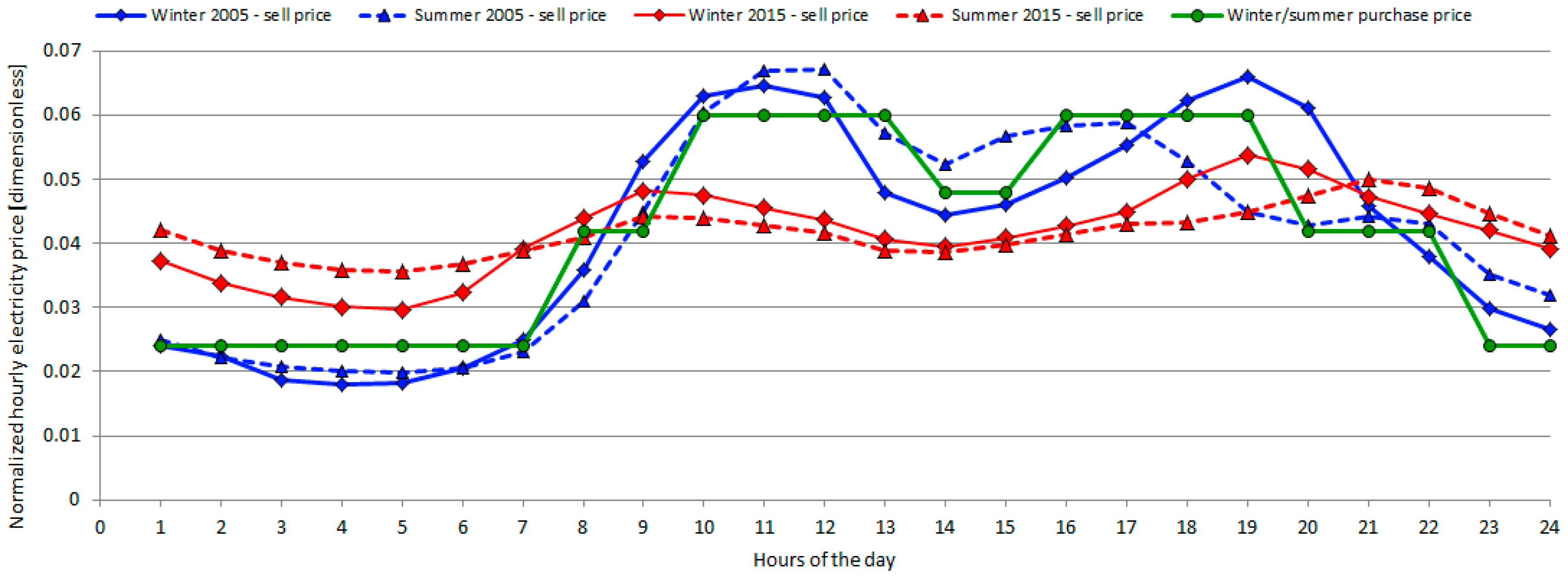
- In 2005 the national power production system essentially relied upon new generation combined cycle power plants, with obsolete steam plants often operated as “hot reserve” and inefficient gas turbines operating, for a limited time, only to supply peak loads. The penetration of renewable was moderately low, with a large prevalence of “predictable production” units like hydropower plants. This mix of technologies of course resulted in high daily fluctuations of electricity prices between peak and off-peak hours;
- -
- In 2015 the national power production system has observed a dramatic increase in the installed capacity of renewable technologies, which is now higher than 50 GW (accounting for more than 42% of the total installed capacity) and being almost comparable with the annual national peak load, which is approximately 52.5 GW. The new installed renewable capacity has a large prevalence of PhotoVoltaics (PV), more than 19 GW, whose production is obviously limited to peak hours and significantly increases in the summer period. As a consequence, during “peak hours” (i.e., during daytime hours when the national electric demand is highest), large amounts of “green” electricity are available, which have been produced with null or very low operating costs. The effect is intuitive: the daily price profiles have been significantly “smoothed”, with an evident reduction of the ratio between the price observed during peak hours (day-time) and off-peak ones (night-time).
- The average shape of the daily energy prices profiles was calculated in normalized terms, i.e., dividing the hourly prices by a cumulated daily total price, so as to have a series of 24 values (one for each hour) that summed up 1.00. The shape was calculated distinctly for the winter and the summer season, and for both the “base case” (year 2005) and the modified scenario (year 2015). The results obtained are shown in Figure 3. It may be observed that in 2005 the ratio between peak and off-peak prices assumed values in the order of 3.5, while in 2015 it is approximately equal to 1.7, thus confirming the aforementioned smoothing effect induced by the high penetration of photovoltaics;
- The normalized profiles derived for 2015 were adopted to develop a new array (with 8760 hourly energy price), but maintaining the same average seasonal electricity prices observed at 2005. In this way, the base case and the newly obtained “modified price profile” only differ for the shape of the daily profile, and not for the average price.
3.2.2. Variation in the Ratio between Electricity and Fuel Price
4. Analysis of the Influence of Uncertain Parameters on the CHCP Viability
- −
- Plant superstructure: the optimization tool offers the possibility to perform the optimization on the basis of different superstructures, including several components and distinct plant lay-out configurations. The analysis presented below were obtained for a superstructure including: (i) a natural gas-fuelled reciprocate engine; (ii) an indirectly-fired double effect absorption chiller; (iii) a non-pressurized heat storage tank, designed to store hot water at 85 °C;
- −
- Width of the temporal basis: in order to limit the computational effort, the optimizations were performed for a “standard year” consisting of 180 days and 24 h per day (i.e., 180 × 24 = 4320 h per year), extracted from the whole set of data (i.e., 8760 h per year) by a well-established procedure [29]. Such a temporal basis, much larger than any of the temporal basis adopted in the referenced works on the same topic [14,18], guarantees that the achieved results are absolutely stable and approximately coincident with those obtainable by adopting a whole set of 8760 hourly data for energy loads and prices.
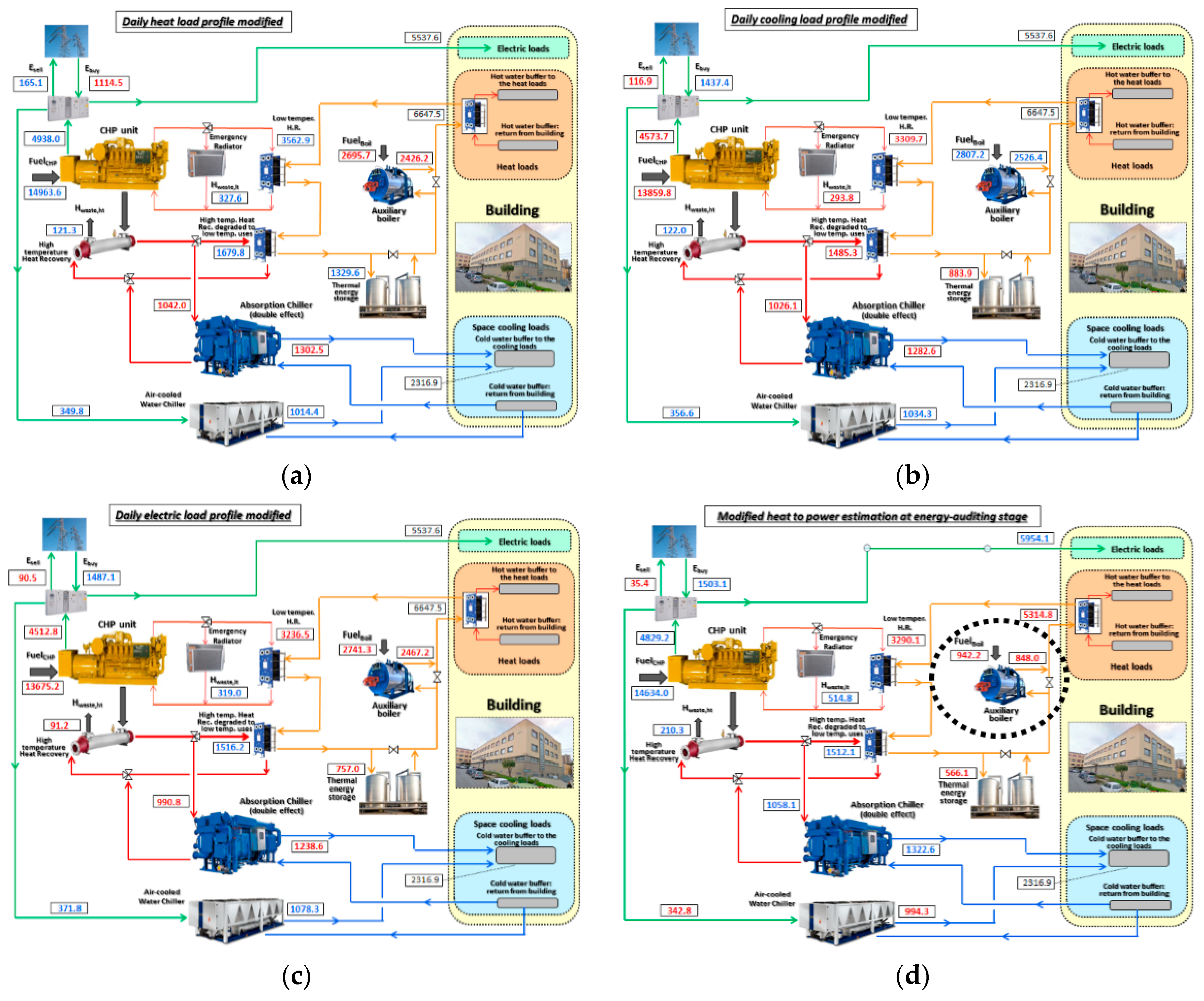
4.1. Results for the Scenarios Including a Single Type of Estimation Error
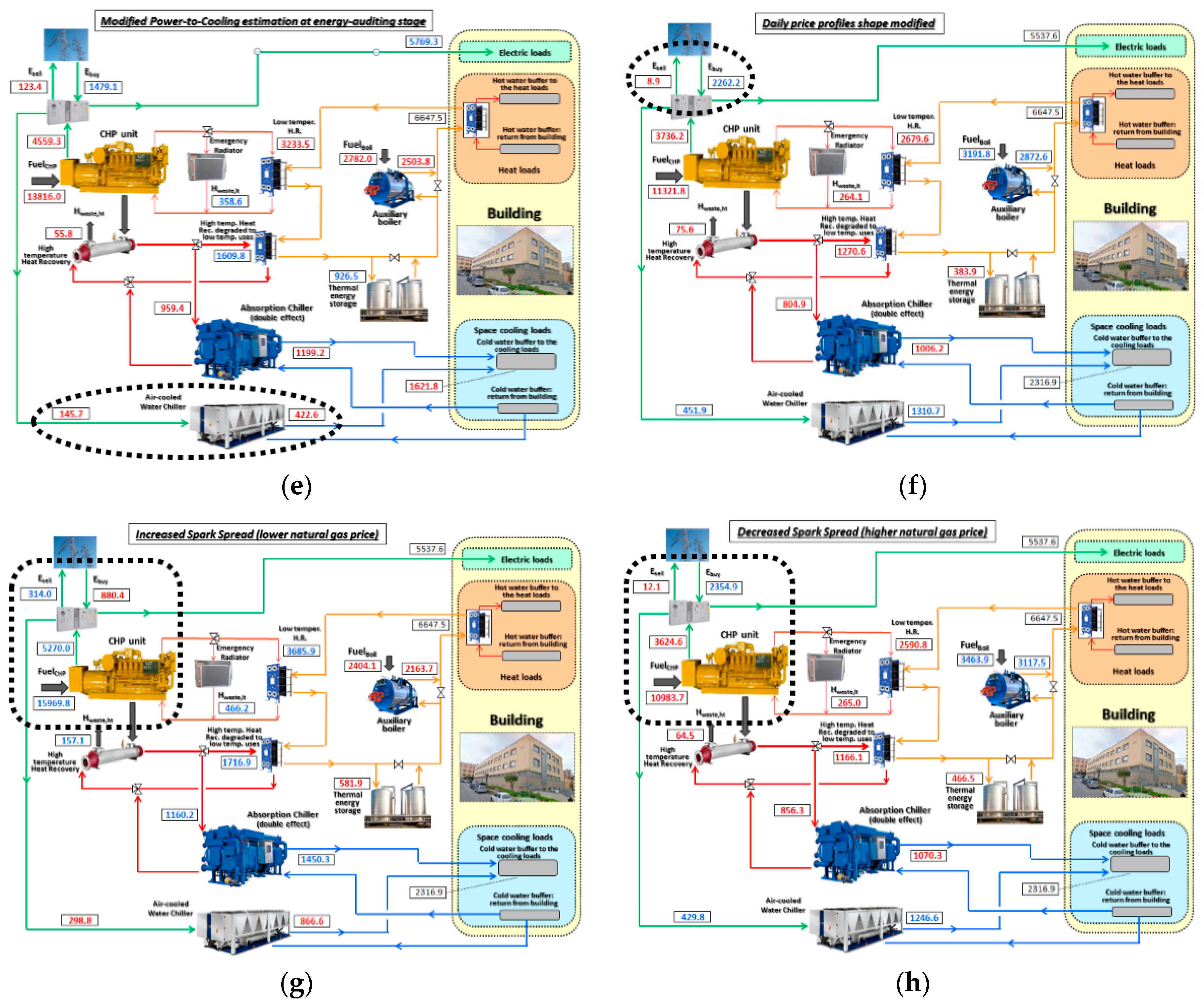
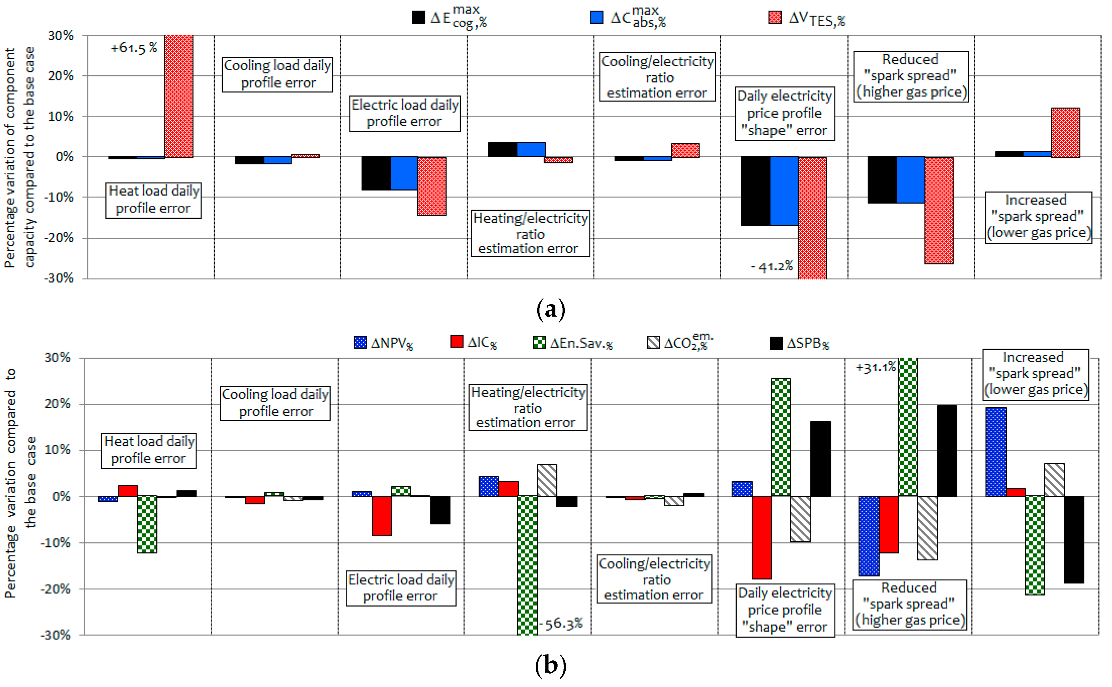
- The optimal capacity of the main plant components remains quite stable (see Figure 4a), assuming for many of the examined “estimation errors” values in the range ±10% compared to the optimal size obtained for the “base case”. Only in a few cases major deviations occur. In particular, as concerns the size of the prime mover, that is the most important component (in terms of investment cost and influence on the operational results), a significant variation in the Spark Spread can modify its optimal size; in particular, for the scenario based on a higher gas price, the reduced profitability of CHP/CHCP operation would make convenient to reduce by more than 10% the size of the engine. Similarly, the shape of the daily electricity price profile seems to be a very critical parameter, since the scenario based on a modified price profile (referring to the year 2015, see red lines in Figure 3) achieved the highest deviations in the optimal size/capacity of all the main plant components. The reason for this behaviour has been partially anticipated in Section 3.2.1: when daily price profiles are quite “flat”, and the price peaks during daytime hours are moderate, the CHP/CHCP plant no longer benefits of the building peak load occurring during daytime hours. Finally, a number of factors significantly influence the optimal size of the Thermal Energy Storage. The charging/discharging phases of TES operation, in fact, are usually optimized so as to allow the CHP unit to produce as much as possible the electricity during “high price” hours, regardless of the high or low heat load in the same hours. The heat eventually recovered and not required by the building users, is stored and supplied later, when needed. It is evident that any distortion in the heat load or in the price profiles can significantly modify the need for such a load shifting and, consequently, the optimal TES capacity;
- The Net Present Value, or the Net Total Cost, is scarcely influenced by all of the examined parameters, but the Spark Spread (see last two series of data in Figure 4b). The strong influence of SS on the viability of CHP unit is absolutely obvious, and represents a well-established principle in literature. A new information, however, emerges from an analysis of Figure 4b: the economic results achieved by the CHP/CHCP unit are negligibly influenced by eventual estimation errors concerning the daily profiles of energy loads and, to some extent, the average power to heat and power to cooling ratios of the user in the winter and summer period. Similar trends may be observed for the Simple PayBack time, SPB;
- The Energy Saving, En.Sav., whose variations are also presented in Figure 4b, is calculated by the following expression:
- -
- In the three scenarios developed by imposing modifications in the daily heat, cooling and electric load profiles, all the annual energy flows observe quite low deviations from the corresponding values observed in the base case. This result again testifies that the adoption of daily “standard” load profiles in order to distribute, on hourly basis, any consumption data eventually available at aggregate monthly or weekly basis is not a critical step in the analysis. Then, the creation of such standard load profiles does not deserve particular efforts, being not necessary to extrapolate very reliable curves;
- -
- The scenarios that assume major changes in the heating to electric and the cooling to electric loads, observe dramatic reductions in the energy supply by the backup units (respectively, the boiler in the former scenario, see Figure 6d, and the vapour compression chiller in the latter one, see Figure 6e), while the heat or cooling supply by the CHP unit and by the absorption chiller are scarcely influenced. An easy interpretation for this result may be given: as both these scenarios assume the same reference prices as the base case, it is evident that in a certain number of hours the combined power and heat/cooling production achieves relevant margins of profitability, and in such hours the optimal load level of the aforementioned units remains unmodified (regardless of the hourly heat to power or heat to cooling load ratio);
- -
- A modification in the shape of the daily electricity price profile induces a dramatic change in the energy balance with the grid. Compared to the results achieved in the base case, when the modified price profile is adopted the amount of energy sold to the grid significantly reduces and, conversely, the purchased electricity increases by a factor 1.65;
- -
- Major changes in the energy exchange with the grid are also observed for the two scenarios obtained for the higher and the lower value of the Spark Spread. Differently than in the previous case, however, the changes imposed in the CHP/CHCP profitability here induces, as a first effect, a dramatic change in the energy production by the CHP unit. The changes in the energy balance with the grid is only a secondary effect, provoked by the changes in the CHP electricity. This result is also confirmed by the much higher (lower) contribution given by the backup components, i.e., the boiler and the vapour compression chiller, for the scenario assuming a lower (higher) value of the Spark Spread.
4.2. Results for Scenarios Including Different Simultaneous Estimation Errors
- -
- The trends show a sort of linearity, in the sense that in presence of several simultaneous estimation errors, the effects induced on the optimal size of components and on the operational results are quite close to the sum of the effects induced, separately, by each effect. This is evident when comparing the first set of data in Figure 7a (case “Simultaneous error in all the daily load profiles”) with the first three sets of data in Figure 4a. Then, there is no “amplificative effect” of each possible estimation error on the effects induced by the other ones;
- -
- The effect induced by estimation error in the Spark Spread seems someway dominant compared to the effects induced by the other errors. For instance, in Figure 7d it may be observed that whatever the combination of errors related with the energy loads and the shape of daily electricity price profiles, the lower margins of profitability guaranteed in case of a lower Spark Spread imply a significant negative deviation of the Net Present Value and an increase in the Simple Payback Time, compared to the base case.
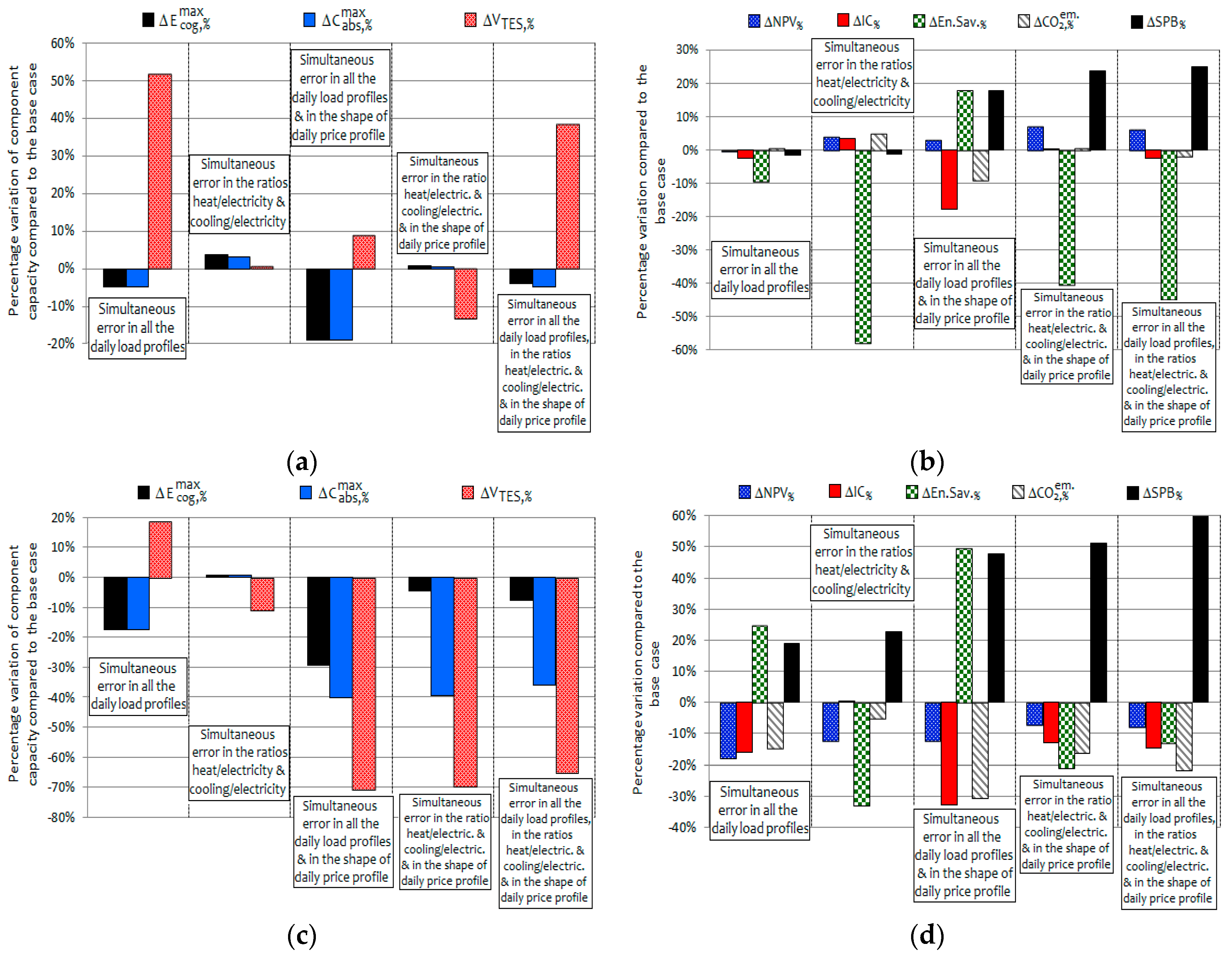
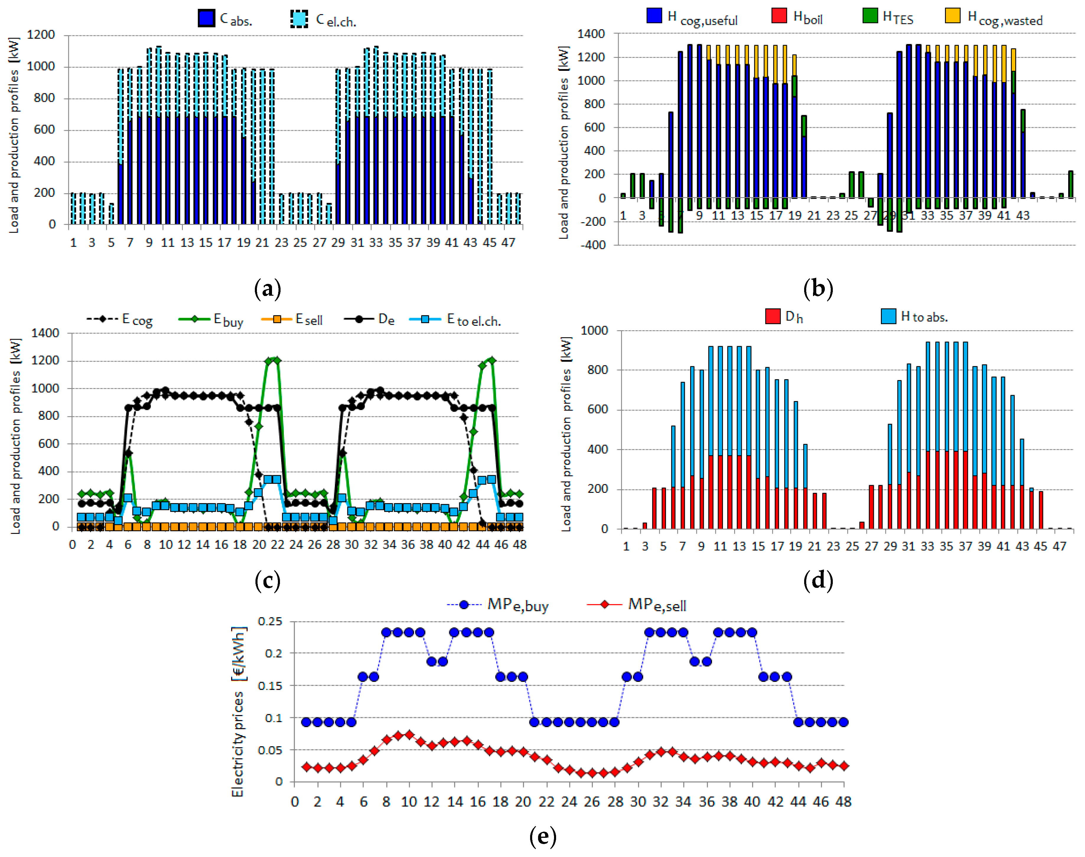
- -
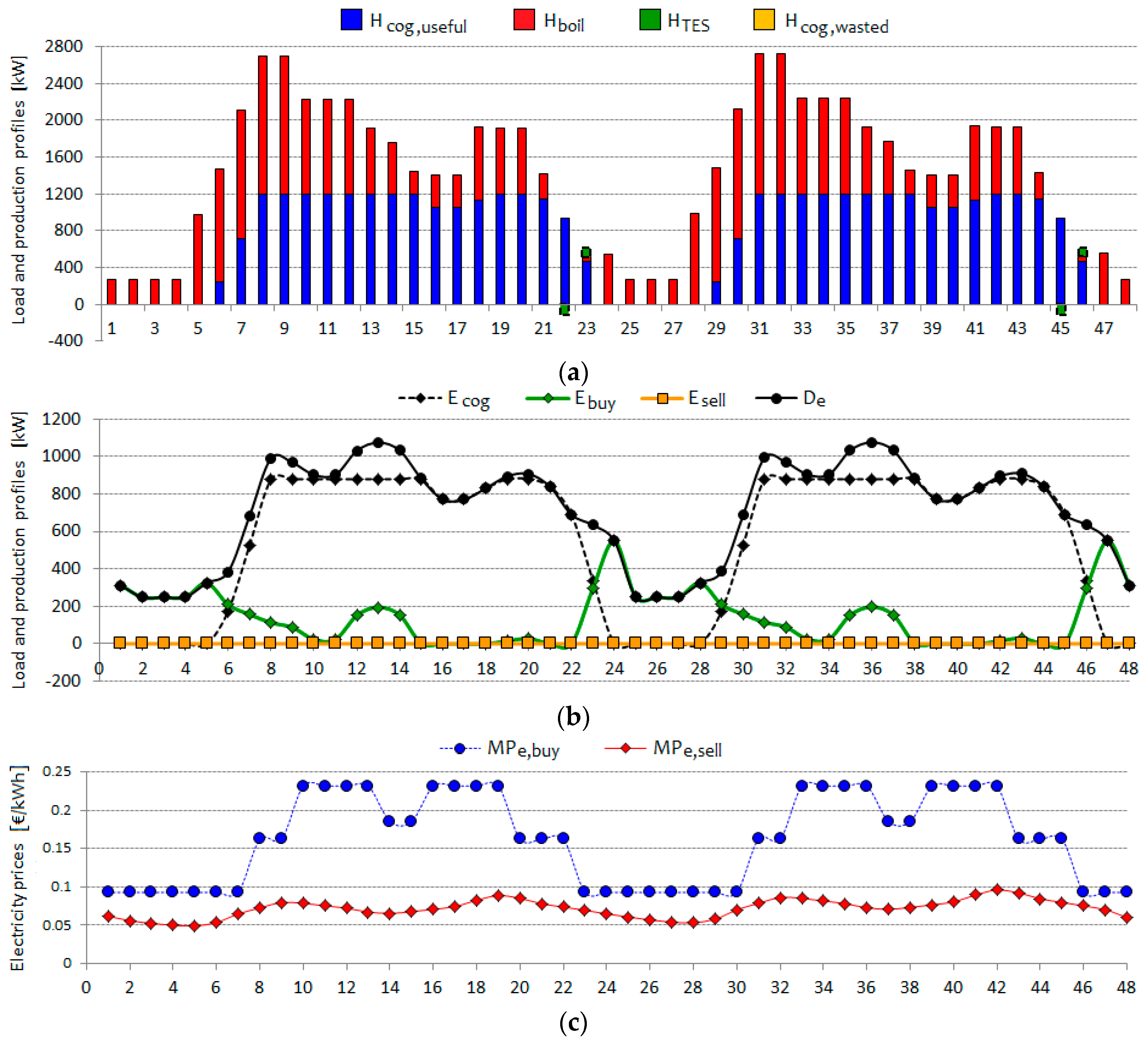
- the CHP unit operates at almost full load for most of the daytime hours, which coincide with the energy price peaks;
- -
- the heat recovery from the engine approximately covers half of the heat demand during winter days. The TES is not used and no heat is wasted. During winter days, the produced electricity is always sufficient to supply the building loads, and some surplus electricity is sold to the grid during peak hours;
- -
- during summer days, the absorption chiller supplies more than 65% of the cooling load. The boiler never operates, since some surplus heat is produced and stored, with moderate amounts being wasted through hot gases and the emergency radiator. In summer no surplus electricity is produced nor sold; conversely, when the energy prices go down during the evening, the engine is switched off and significant amounts of electricity are purchased from the grid. Finally, looking at the heat uses (see Figure 9d), more than half of the heat demand is related with “indirect heat uses”, i.e., to supply the absorption chiller.
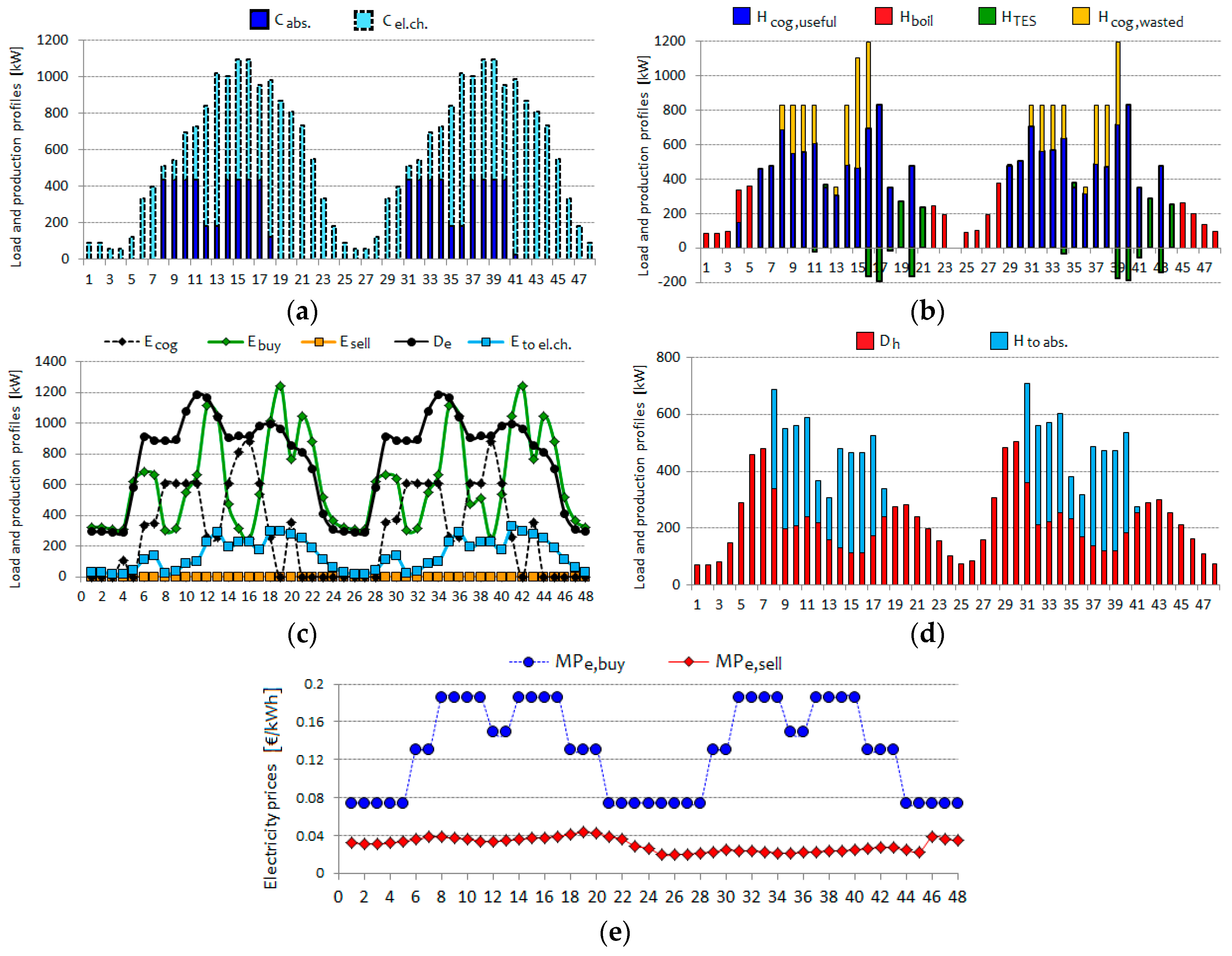
- -
- In the winter period, the optimal plant operation observes only slight changes, mainly related with the operation of the backup boiler which must now supply additional heat to follow a different daily load profile. Conversely, major modifications are observed as concerns the electricity balance: differently than in the base case, in the “modified scenario” the system never produces surplus electricity to be sold to the grid, while low amounts of energy are purchased during off-peak hours. An interpretation for this last trend is intuitive: due to the reduced price peaks during peak hours (related with the “flat” daily energy sell price profile assumed in the modified scenario), operating the CHP unit during peak hours so as to produce surplus electricity to be sold is no longer convenient. As concerns the role of the Thermal Energy Storage, in the modified scenario it provides an almost null contribute to the heat balance, exactly like in the base case. Also, the optimal operation in the modified scenario does not assume any amount of heat to be wasted, exactly as observed in the base case;
- -
- More articulate analyses are needed for the summer case, where the differences between the optimal operation obtained for the base case (see Figure 9a–e) and the modified scenario (see Figure 11a–e) are more complex. First of all, let us compare the CHP electricity production rates presented in Figure 9c and Figure 11c: it may be observed that while in the base case the CHP unit was operated at full load continuously for all the daytime hours, in the modified scenario the optimal operation of the CHP unit is much more discontinuous. Provided that the tool assumes as infeasible any prime mover operating condition with too frequent start-up/shut-down cycles, an interpretation for such an irregular operation may be given. Due to the low margins of profitability, related with the low Spark Spread and with the intrinsically lower economic convenience of combined cooling and power product in summer (compared to the heating and power production in winter), the optimal operation in the modified scenario must ensure that: (i) the energy outputs from the CHP unit are entirely used to supply a useful demand; (ii) the electricity production is self-consumed, so that each kWh of produced electricity generates an “avoided cost” MPe,buy, rather than a revenue MPe,sell (with MPe,sell much lower than MPe,buy). Also, in the modified scenario the absorption chiller supplies a much lower fraction of the cooling demand, compared to the base case.
4.3. Conceptual Achievements of the Proposed Study
- The definition of daily load profiles, in terms of curve “shape”, is not a critical phase and could consequently be paid a moderate effort when conducting the energy audit of an existing building. Indeed, eventual estimation errors concerning daily load profiles will lead to minor errors in sizing the CHP unit and the absorption chiller, with slightly more significant deviations as concerns the optimal size of the heat storage. Also the economic, energetic and environmental results are scarcely sensitive to the assumed heat, cooling and electric load profiles;
- In the analysis of energy loads for existing buildings, when data on the electricity consumption for lighting and appliances and those related with HVAC systems are grouped together (as usual in the energy bills), eventual errors occurring in the allocation of these two kinds of “direct” and “indirect” electricity uses also lead to moderate changes in the optimal CHCP solution. Only in terms of avoided CO2 emissions, eventual estimation error can lead to significant under- or over-estimation due to the different emission factors per kWh of heat, cooling and electricity;
- Erroneous prediction, over the plant life cycle, of the “shape” of daily energy price profiles may induce to rather relevant changes in the optimal size of the main plant components and in the economic and energo-environmental results. This conclusion is someway intuitive, since the economic attractiveness of combined heating, cooling and power production increases whenever most of the energy loads occur during “peak hours”, i.e., hours characterized by higher energy prices;
5. Conclusions
Author Contributions
Conflicts of Interest
Abbreviations and Symbols
| C | Cooling |
| D | Demand or load (kW) |
| DHW | Domestic Hot Water |
| E | Electricity |
| En.Sav. | Energy Saving |
| F | Fuel |
| H | Heat |
| Itot | Total investment cost |
| LHV | Low Heat Value (kJ/Nm3 and kJ/kg, respectively for gaseous and liquid fuels) |
| MP | Market Price (€/kWh or €/Nm3, respectively for electricity and gaseous fuels) |
| Nhours | Number of hours used as temporal basis for the optimization |
| NPV | Net Present Value |
| PHR | Power to Heat Ratio |
| Ref Eη | Reference efficiency for the separate production of electricity |
| SS | Spark Spread |
| STORi | Stored Thermal energy at the beginning of a generic time step “i” |
| V | Volume (m3) |
| Greek letters | |
| δ | Boolean 0–1 variable at plant synthesis level |
| η | Efficiency |
| Subscripts | |
| abs | Absorption chiller |
| boil | Backup boiler |
| cog | Related to the operation of the cogeneration unit |
| TES | Thermal Energy Storage |
| trad | Traditional plant, producing separately electricity, heat and/or cooling |
| Acronyms | |
| CHCP | Combiner Heat, Cooling and Power |
| CHP | Combined Heat and Power, also used to indicate “efficient cogeneration” according to European Directive |
| COP | Coefficient of Performance |
| FEL | Following the Electric Load |
| FTL | Following the Thermal Load |
| HVAC | Heating, Ventilating and Air-Conditioning |
| MILP | Mixed Integer Linear Programming |
| MINLP | Mixed Integer NonLinear Programming |
| PGU | Power Generation Unit |
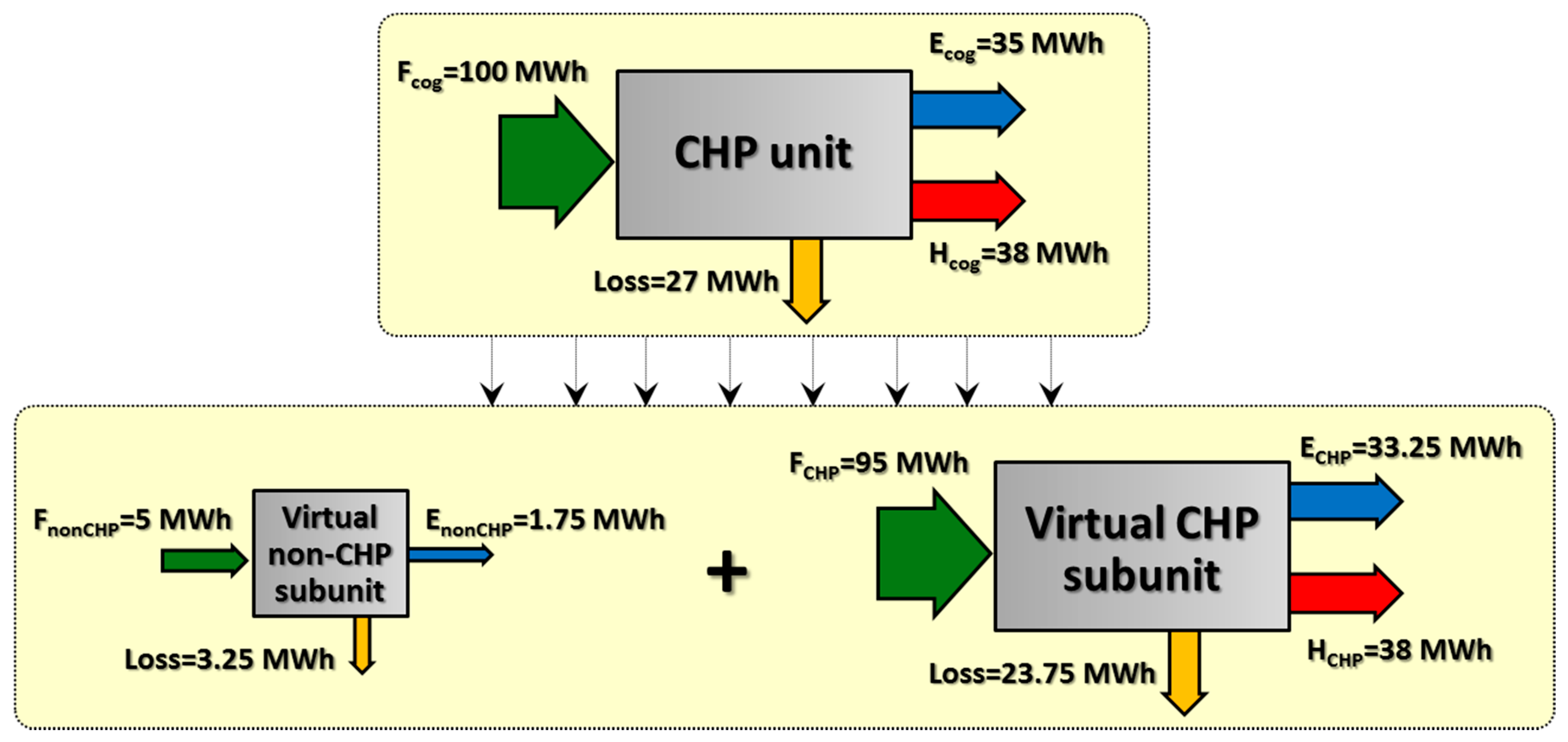
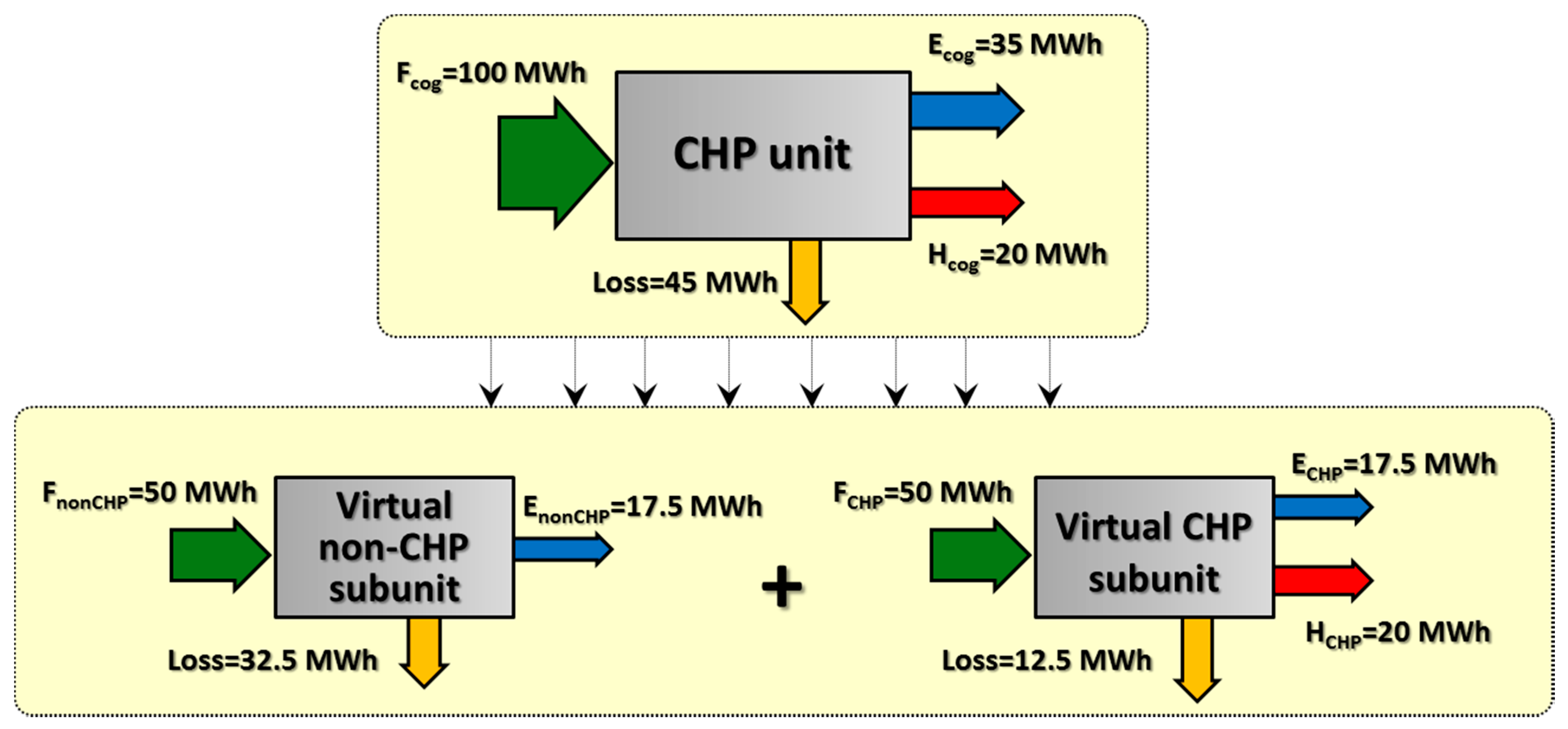
Appendix A
- -
- the plant achieving a higher efficiency is decomposed into a large CHP subunit and a very small nonCHP one;
- -
- the plant achieving a lower energy efficiency is decomposed into two CHP and nonCHP subunits with comparable “sizes”.
References
- Angrisani, G.; Canelli, M.; Roselli, C.; Sasso, M. Microcogeneration in buildings with low energy demand in load sharing application. Energy Convers. Manag. 2015, 100, 78–89. [Google Scholar] [CrossRef]
- Siler-Evans, K.; Granger Morgan, M.; Lima Azevedo, I. Distributed cogeneration for commercial buildings: Can we make the economics work? Energy Policy 2012, 42, 580–590. [Google Scholar] [CrossRef]
- Sanaye, S.; Khakpaay, N. Simultaneous use of MRM (maximum rectangle method) and optimization methods in determining nominal capacity of gas engines in CCHP (combined cooling, heating and power) systems. Energy 2014, 72, 145–158. [Google Scholar] [CrossRef]
- Cardona, E.; Piacentino, A. A methodology for sizing a trigeneration plant in Mediterranean areas. Appl. Therm. Eng. 2003, 23, 1665–1680. [Google Scholar] [CrossRef]
- Wang, J.J.; Bai, H.; Jing, Y.Y.; Zhang, J.L. Economic Analysis and Optimization Design of a Solar Combined Cooling Heating and Power System in Different Operation Strategies. In Proceedings of the 7th IEEE Conference on Industrial Electronics and Applications (ICIEA), Singapore, 18–20 July 2012; pp. 108–112.
- Mauser, I.; Müller, J.; Allerding, F.; Schmeck, H. Adaptive building energy management with multiple commodities and flexible evolutionary optimization. Renew. Energy 2016, 87, 911–921. [Google Scholar] [CrossRef]
- Anvari, S.; Taghavifar, H.; Khoshbakhti Saray, R.; Khalilarya, S.; Jafarmada, S. Implementation of ANN on CCHP system to predict trigeneration performance with consideration of various operative factors. Energy Convers. Manag. 2015, 101, 503–514. [Google Scholar] [CrossRef]
- Rong, A.; Lahdelma, R. An efficient linear programming model and optimization algorithm for trigeneration. Appl. Energy 2005, 82, 40–63. [Google Scholar] [CrossRef]
- Andiappan, V.; Ng, K.S.D. Synthesis of tri-generation systems: Technology selection, sizing and redundancy allocation based on operational strategy. Comput. Chem. Eng. 2016, 91, 380–391. [Google Scholar] [CrossRef]
- Arcuri, P.; Beraldi, P.; Florio, G.; Fragiacomo, P. Optimal design of a small size trigeneration plant in civil users: A MINLP (Mixed Integer Non Linear Programming Model). Energy 2015, 80, 628–641. [Google Scholar] [CrossRef]
- Morari, M. Flexibility and resiliency of process systems. Comput. Chem. Eng. 1983, 7, 423–438. [Google Scholar] [CrossRef]
- Larsson, T.; Wene, C.O. Developing strategies for robust energy systems. I: Methodology. Int. J. Energy Res. 1993, 17, 503–513. [Google Scholar] [CrossRef]
- Lai, S.M.; Hui, C.W. Feasibility and flexibility for a trigeneration system. Energy 2009, 34, 1693–1704. [Google Scholar] [CrossRef]
- Lai, S.M.; Hui, C.W. Integration of trigeneration system and thermal storage under demand uncertainties. Appl. Energy 2010, 87, 2868–2880. [Google Scholar] [CrossRef]
- Gamou, S.; Yokoyama, R.; Ito, K. Optimal unit sizing of cogeneration systems in consideration of uncertain energy demands as continuous random variables. Energy Convers. Manag. 2002, 43, 1349–1361. [Google Scholar] [CrossRef]
- Gamou, S.; Yokoyama, R.; Ito, K. Optimal sizing of cogeneration systems under the toleration for shortage of energy supply. Int. J. Energy Res. 2000, 24, 61–75. [Google Scholar] [CrossRef]
- Hu, M.; Cho, H. A probability constrained multi-objective optimization model for CCHP system operation decision support. Appl. Energy 2014, 116, 230–242. [Google Scholar] [CrossRef]
- Ersoz, I.; Colak, U. Combined cooling, heat and power planning under uncertainty. Energy 2016, 109, 1016–1025. [Google Scholar] [CrossRef]
- Li, C.Z.; Shi, Y.M.; Huang, X.H. Sensitivity analysis of energy demands on performance of CCHP system. Energy Convers. Manag. 2008, 49, 3491–3497. [Google Scholar] [CrossRef]
- Li, C.Z.; Shi, Y.M.; Liu, S.; Zheng, Z.L.; Liu, Y.C. Uncertain programming of building cooling heating and power (BCHP) system based on Monte-Carlo method. Energy Build. 2010, 42, 1369–1375. [Google Scholar] [CrossRef]
- Smith, A.; Luck, R.; Mago, P.J. Analysis of a combined cooling, heating and power system model under different operating strategies with input and model data uncertainty. Energy Build. 2010, 42, 2231–2240. [Google Scholar] [CrossRef]
- Akbari, K.; Nasiri, M.M.; Jolai, F.; Ghaderi, S.F. Optimal investment and unit sixing of distributed Energy systems under uncertainty: A robust optimization approach. Energy Build. 2014, 85, 275–286. [Google Scholar] [CrossRef]
- Wang, L.; Singh, C. Stochastic combined heat and power dispatch based on multi-objective particle swarm optimization. Int. J. Electr. Power 2008, 30, 226–234. [Google Scholar] [CrossRef]
- Carvalho, M.; Lozano, M.A.; Ramos, J.; Serra, L.M. Synthesis of trigeneration systems: Sensitivity analyses and resilience. Sci. World J. 2013, 2013, 604752. [Google Scholar] [CrossRef] [PubMed]
- Carpaneto, E.; Chicco, G.; Mancarella, P.; Russo, A. Cogeneration planning under uncertainty. Part I: Multiple time frame approach. Appl. Energy 2011, 88, 1059–1067. [Google Scholar] [CrossRef]
- Carpaneto, E.; Chicco, G.; Mancarella, P.; Russo, A. Cogeneration planning under uncertainty. Part II: Decision theory-based assessment of planning alternatives. Appl. Energy 2011, 88, 1075–1083. [Google Scholar] [CrossRef]
- Ortiga, J.; Bruno, J.C.; Coronas, A. Selection of typical days for the characterisation of energy demand in cogeneration and trigeneration optimisation models for buildings. Energy Convers. Manag. 2011, 52, 1934–1942. [Google Scholar] [CrossRef]
- Piacentino, A.; Barbaro, C. A comprehensive tool for efficient design and operation of polygeneration-based energy μgrids serving a cluster of buildings. Part II: Analysis of the applicative potential. Appl. Energy 2013, 111, 1222–1238. [Google Scholar] [CrossRef]
- Piacentino, A.; Barbaro, C.; Cardona, F.; Gallea, R.; Cardona, E. A comprehensive tool for efficient design and operation of polygeneration-based energy μgrids serving a cluster of buildings. Part I: Description of the method. Appl. Energy 2013, 111, 1204–1221. [Google Scholar] [CrossRef]
- LINDO API 8.0 User Manual; LINDO System, Inc.: Chicago, IL, USA, 2013.
- Cardona, E.; Piacentino, A. DABASI—WWW Promotion of Energy Savings by CHCP Plants, Database and Evaluation. Final Report; Project Financed within the EU SAVE Programme, Contract No. 4.1031/Z/02-060; Project Consortium: Bruxelles, Belgium, 2005. [Google Scholar]
- Environmental Protection Agency e Combined Heat and Power Partnership Program, Report “Technology Characterization: Reciprocating Engines”. Available online: http://www.epa.gov/chp/documents/catalog_chptech_reciprocating_engines.pdf (accessed on 10 February 2014).
- Directive 2004/8/EC of the European Parliament and of the Council of 11 February 2004 on the promotion of cogeneration based on a useful heat demand in the internal energy market and amending Directive 92/42/EEC. Off. J. Eur. Union 2004, 52, 50–60.
- Cardona, E.; Culotta, S. CHOSE—Energy Saving by Combined Heat, Cooling and Power Plants in the Hotel Sector. Final Report; Project Financed within the SAVE II Programme, Contract No. XVII/4.1031/Z/98-036; Project Consortium: Bruxelles, Belgium, 2001. [Google Scholar]
- Gestore dei Mercati Energetici. Available online: http://www.mercatoelettrico.org/It/Download/DatiStorici.aspx (accessed on 27 September 2016).
- Angrisani, G.; Akisawa, A.; Marrasso, E.; Roselli, C.; Sasso, M. Performance assessment of cogeneration and trigeneration systems for small scale applications. Energy Convers. Manag. 2016, 125, 194–208. [Google Scholar] [CrossRef]
- Kavvadias, K.C. Energy price spread as a driving force for combined generation investments: A view on Europe. Energy 2016, 115, 1632–1639. [Google Scholar] [CrossRef]
- Smith, A.D.; Fumo, N.; Mago, P.J. Spark spread e a screening parameter for combined heating and power systems. Appl. Energy 2011, 88, 1494–1499. [Google Scholar] [CrossRef]
- Chicco, G.; Mancarella, P. Assessment of the greenhouse gas emissions from cogeneration and trigeneration systems. Part I: Models and indicators. Energy 2008, 33, 410–417. [Google Scholar] [CrossRef]
- European Commission. Commission Decision establishing harmonized efficiency reference values for separate production of electricity and heat in application of Directive 2004/8/EC. Off. J. Eur. Union 2007, 32, 183–188. [Google Scholar]


© 2016 by the authors; licensee MDPI, Basel, Switzerland. This article is an open access article distributed under the terms and conditions of the Creative Commons Attribution (CC-BY) license (http://creativecommons.org/licenses/by/4.0/).
Share and Cite
Piacentino, A.; Gallea, R.; Catrini, P.; Cardona, F.; Panno, D. On the Reliability of Optimization Results for Trigeneration Systems in Buildings, in the Presence of Price Uncertainties and Erroneous Load Estimation. Energies 2016, 9, 1049. https://doi.org/10.3390/en9121049
Piacentino A, Gallea R, Catrini P, Cardona F, Panno D. On the Reliability of Optimization Results for Trigeneration Systems in Buildings, in the Presence of Price Uncertainties and Erroneous Load Estimation. Energies. 2016; 9(12):1049. https://doi.org/10.3390/en9121049
Chicago/Turabian StylePiacentino, Antonio, Roberto Gallea, Pietro Catrini, Fabio Cardona, and Domenico Panno. 2016. "On the Reliability of Optimization Results for Trigeneration Systems in Buildings, in the Presence of Price Uncertainties and Erroneous Load Estimation" Energies 9, no. 12: 1049. https://doi.org/10.3390/en9121049