
Research and Application of a Hybrid Forecasting Model Based on Data Decomposition for Electrical Load Forecasting


Abstract
:1. Introduction
- Improve the social and economic benefits. The electrical power sector is supposed to ensure a good social benefit through providing safe and reliable electricity and improving the economic benefits considering the cost problems. Thus, the electrical load forecasting is beneficial for electrical power system to achieve the economic rationality of power dispatching.
- Ensure the reliability of electricity supply. Whether the power generation or supply, equipment needs periodical overhauls to ensure the safety and reliability of electricity. However, when to overhaul or replace the equipment should be based on accurate electrical load forecasting results.
- Plan for electrical power construction. The construction of electrical power production sites cannot stay unchanged, and should be adjusted and perfected, to satisfy the demands of a constantly changing future with the progress of society and development of the economy.
- Long-term electrical load forecasting. This means a time interval above five years and is usually conducted during the planning and building stage of the electrical system, which considers the characteristics of the electrical system and the development tendencies of the national economy and society;
- Middle-term electrical load forecasting. It is mainly applied in the operation stage of the electrical power system, for direction of the scientific dispatch of power, arrangement of overhauling and so on;
- Short-term electrical load forecasting. It plays a pivotal role in the whole electrical system and is the most important part, for it is the basis of long- and middle-term electrical load forecasting. Besides, it can ensure the stable and safe operation of the electrical power system based on the forecasting data.
- (1)
- The time series data have the characteristics of continuity, periodicity, trend and randomness, and considerable work has been done to select suitable models and the optimize the model parameters; however, few studies focus on building forecasting models based on the characteristics of the time series data. Therefore, the initial contribution of this paper is to decompose the time series data. Based on the traditional additive model, the layer-upon-layer decomposition and reconstitution method is applied to improve the forecasting accuracy. Then according to the data features after decomposition, suitable models could be found to perform the forecasting. Through effective decomposition of the data and selection of reasonable model, the forecasting quality and accuracy could be improved to a great degree.
- (2)
- This paper uses the generalized regression neural network (GRNN) to improve the forecasting performance. The data after decomposition have noises, so the empirical mode decomposition (EMD) is applied to reduce the noise in the data. Then the genetic algorithm (GA) is utilized to optimize the GRNN to conduct the forecasting to enhance the forecasting accuracy of the single model.
- (3)
- The practical application of the proposed hybrid model in this paper is to forecast the short-term electrical load in New South Wales of Australia, and compare it with the single models and models without decomposition. The forecasting results demonstrate that the proposed model has a strong non-linear fitting ability and good forecasting quality for electrical load time series. Both the simulation results and the forecasting process could fully show that the hybrid model based on the data decomposition has the features of small errors and fast speed. The algorithm applied in the electrical power system is not only applicable, but also effective.
2. Methods
2.1. Additive and Multiplicative Model of Time Series
2.2. Moving Average Model
2.3. Periodic Adjustment Model
2.4. Empirical Mode Decomposition
| Algorithm 1: Pseudo code of Empirical Mode Decomposition |
| Input: —a sequence of sample data. Output: —a sequence of denoising data. |
| Parameters: |
| —represent a random number in the algorithm with the value between 0.2 and 0.3. |
| T—a parameter describing the length of the original electrical load time series data. |
| 1: /*Initialize residue ; Extract local maxima and minima of .*/ 2: FOR EACH (j = j + 1) DO 3: FOR EACH () DO 4: WHILE (Stopping Criterion ) DO 5: Calculate the upper envelope Ui(t) and Li(t) via cubic spline interpolation. 6: /* Mean envelope */; hi(t) = ri−1(t) − mi(t)/* ith component */ 7: /*Let hi,j(t) = hi(t), with mi,j(t) being the mean envelope of hi,j(t)*/ 8: END WHILE 9: Calculate 10: /*Let the jth IMF be IMFi(t) = hi,j(t); Update the residue ri(t) = ri−1(t) − IMFi(t)*/ 11: END DO 12: END DO 13: Return /* The noise reduction process is finished */ |
2.5. Generalized Regression Neural Network (GRNN)
3. The Proposed Hybrid Model
3.1. Genetic Algorithm
| Algorithm 2: Pseudo Code of the genetic algorithm |
| Input: —a sequence of training data —a sequence of verifying data Output: fitness_value xb—the value with the best fitness value in the population of populations Parameters: Genmax—the maximum number of iterations; n—the number of individuals Fi—the fitness function of the individual i; xi—the population i g—the current iteration number of GA; d—the number of dimension 1: /*Initialize the population of n individuals which are xi\(i = 1, 2, ..., n) randomly.*/ 2: /*Initialize the parameters of GA: Initial probabilities of crossover pc and mutation pm.*/ 3: FOR EACH (i: 1 ≤ i ≤ n) DO 4: Evaluate the corresponding fitness function Fi 5: END FOR 6: WHILE (g < Genmax) DO FOR EACH (I = 1:n) DO 7: IF (pc > rand) THEN 8: /*Conduct the crossover operation*/ and 9: END IF 10: IF (pm > rand) THEN 11: /*Conduct the Mutate operation*/ 12: END IF END FOR 13: FOR EACH (i: 1 ≤ i ≤ n) DO 14: Evaluate the corresponding fitness function Fi 15: END FOR 16: /*Update the best nest xp of the d generation in the genetic algorithm.*/ 17: FOR EACH (i: 1 ≤ i ≤ n) DO IF (Fp< Fb) THEN 18: /* The global best solution can be obtained to replace the local optimal xb←xp*/ 19: END IF END FOR END WHILE 20: RETURN xb/* The optimal solution in the global space has been obtained.*/ |
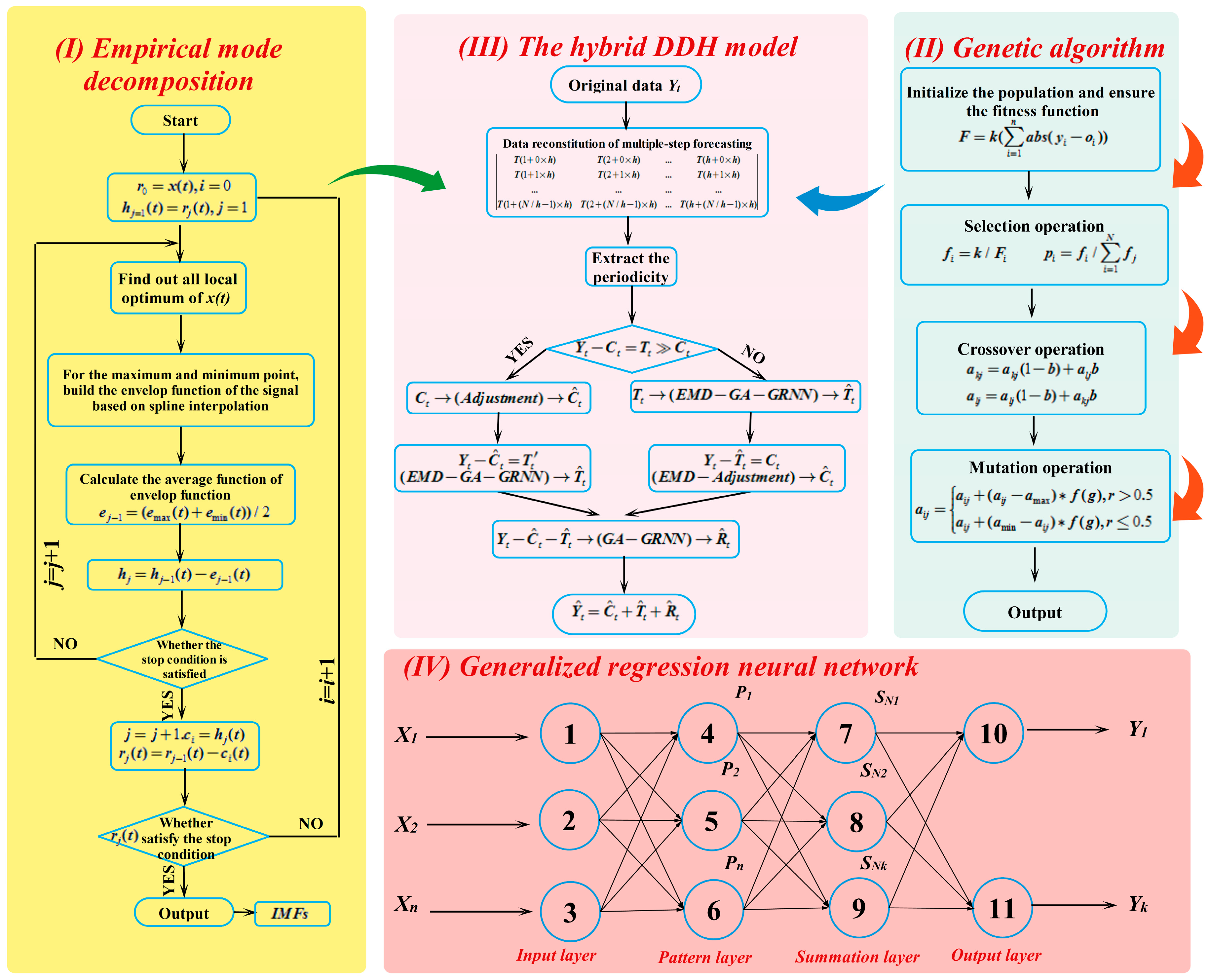
3.2. Data Decomposition Hybrid (DDH) Model
3.3. The EMD-GA-GRNN Forecasting Model
| Algorithm 3: Pseudo code of the hybrid model of EMD-GA-GRNN |
| Input: —a sequence of training data —a sequence of verifying data Output: —forecasting electrical load from GRNN Fitness function: /*The objective fitness function*/ Parameters: Genmax—the maximum number of iterations; n—the number of individuals Fi—the fitness function of individual i; xi—the total population i G—the current iteration number; d—the number of dimension 1: /* Process original electrical load time series data with the noise reduction method EMD */ 2: /*Initialize the population of n individuals xi (i = 1, 2, ..., n) randomly.*/ 3: /*Initialize the original parameters: Initial probabilities of crossover pc and mutation pm.*/ 4: FOR EACH (i: 1 ≤ i ≤ n) DO 5: Evaluate the corresponding fitness function Fi 6: END FOR 7: WHILE (g < Genmax) DO 8: FOR EACH (i = 1:n) DO IF (pc > rand) THEN 9: Conduct the crossover operation of GA to optimize the smoothing factor of GRNN 10: END IF 11: IF (pm > rand) THEN 12: Conduct the mutate operation of GA to optimize the smoothing factor of GRNN 13: END IF END FOR 14: FOR EACH (i: 1 ≤ i ≤ n) DO 15: Evaluate the corresponding fitness function Fi 16: END FOR 17: /*Update best nest xp of the d generation to replace the former local optimal solution.*/ 18: FOR EACH (i: 1 ≤ i ≤ n) DO IF (Fp < Fb) THEN xb←xp; 19: END IF END FOR END WHILE 20: RETURN xb/* Set the weight and threshold of the GRNN according to xb.*/ 21: Use xt to train the GRNN and update the weight and threshold of the GRNN and input the historical data into GRNN to obtain the forecasting value . |
4. Experiments
4.1. Model Evaluation
- (1)
- Selection of influencing factors when constructing mathematical models. In truth, the time series is affected by various factors, and it is difficult to master all of them. Therefore, errors between forecast values and actual values cannot be avoided.
- (2)
- Improper algorithms. For forecasting, we just build a relatively appropriate model, so if the algorithms are chosen wrongly, the errors would become larger.
- (3)
- Inaccurate or incomplete data. The forecasting should be based on the historical data, so inaccurate or incomplete data can result in forecasting errors.
4.2. Experimental Setup
- (1)
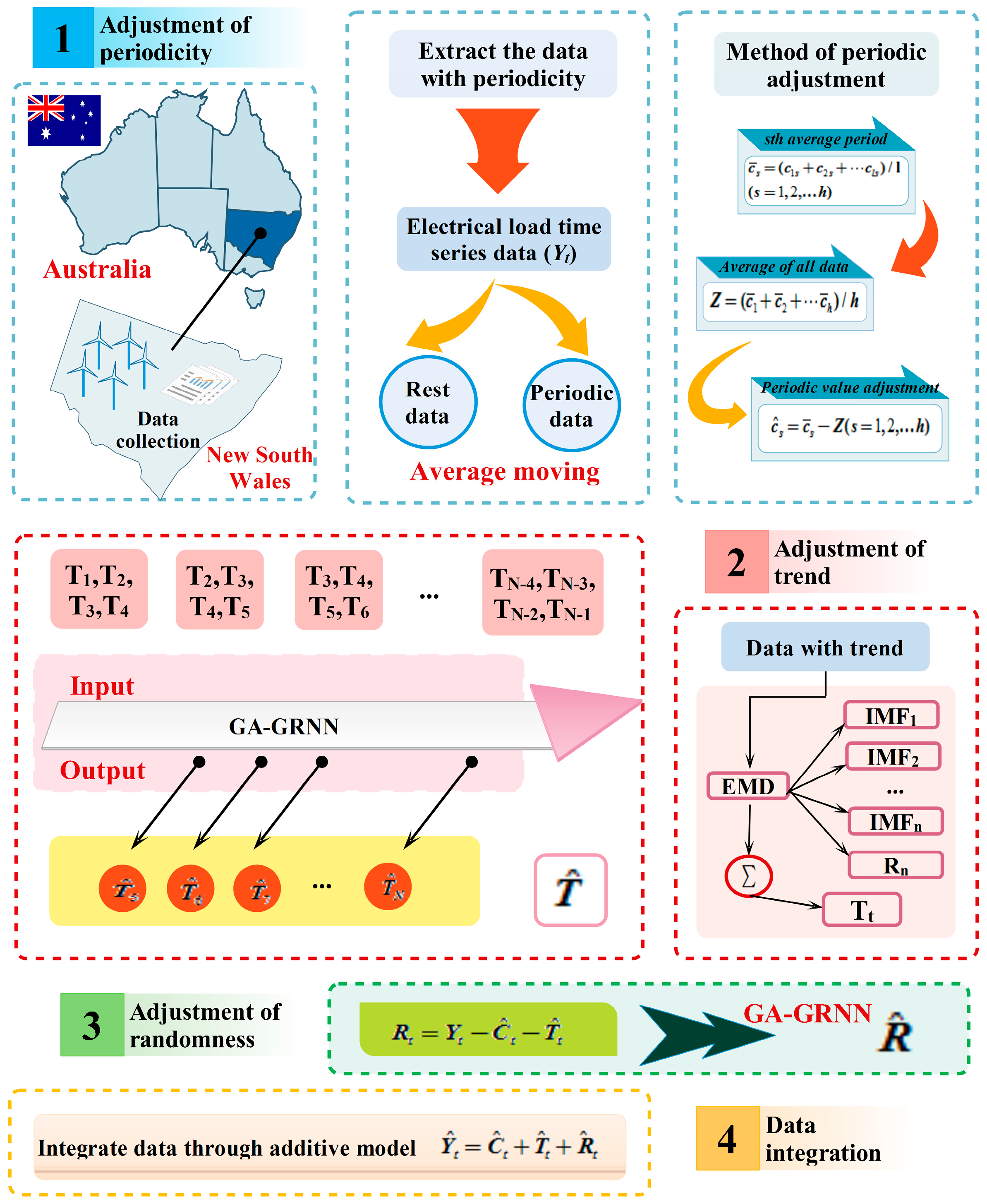
- The original electrical load time series data has an obvious trend and periodicity. Initially, the moving average method is conducted to extract the periodicity . For the periodicity , conduct the periodic adjustment and obtain .
- (2)
- Subtract the periodicity of the original time series data, and get the original trend (). For the original data without periodicity, EMD needs to be initially applied to eliminate the noises and improve the forecasting accuracy. Then the genetic algorithm could be used to optimize GRNN to obtain the forecasting trend item .
- (3)
- Finally, the randomness can be obtained through , then the GRNN optimized by the genetic algorithms is utilized to forecast the randomness and the forecasting value is obtained. The trend tends to be steady; therefore, there is no need to eliminate noises.
- (4)
- The final forecasting is performed by the additive model of time series .
4.3. Empirical Results
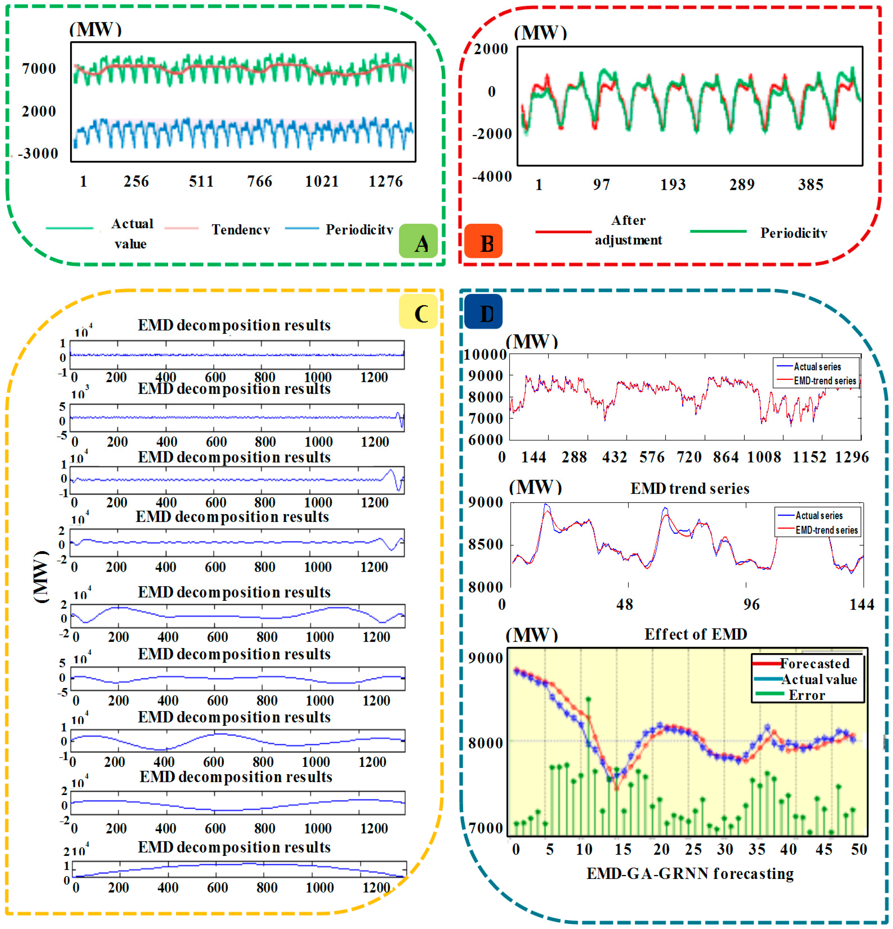
- (1)
- Figure 3A shows the results after decomposition by moving average, from which it can be seen that the original electrical load data contains a certain periodicity, and the variation of the period is roughly equal, so the additive model is more suitable. The length of the period h = 48 can be ensured based on the data distribution. Thus the moving average method is used to decompose the electrical load data into two parts, which are periodicity and trend. Besides, from the decomposed results, it can be known that the level of trend is nearly ten times the periodicity. This is because that the moving average method can demonstrate the large trend of the development, eliminating the fluctuation factors such as season. Therefore, the periodic adjustment should be conducted through extracting the periodicity.
- (2)
- Figure 3B is the electrical load data after periodic adjustment, from which is can be known that the electrical load data after the periodic adjustment have periodic sequence and basis trend characteristics.
- (3)
- Figure 3C demonstrates the output results of trend data after EMD. It shows that nine components are obtained, including IMF1, IMF2, …, IMF8 and Rn, after EMD data decomposition. The high-frequency data in highest component is removed, and the rest data are regarded as the new trend time series data.
- (4)
- Figure 3D clearly reveals the trend data after EMD decomposition by removing the high frequency component, and it can be obviously seen that the data denoised by EMD are smoother than the original data.
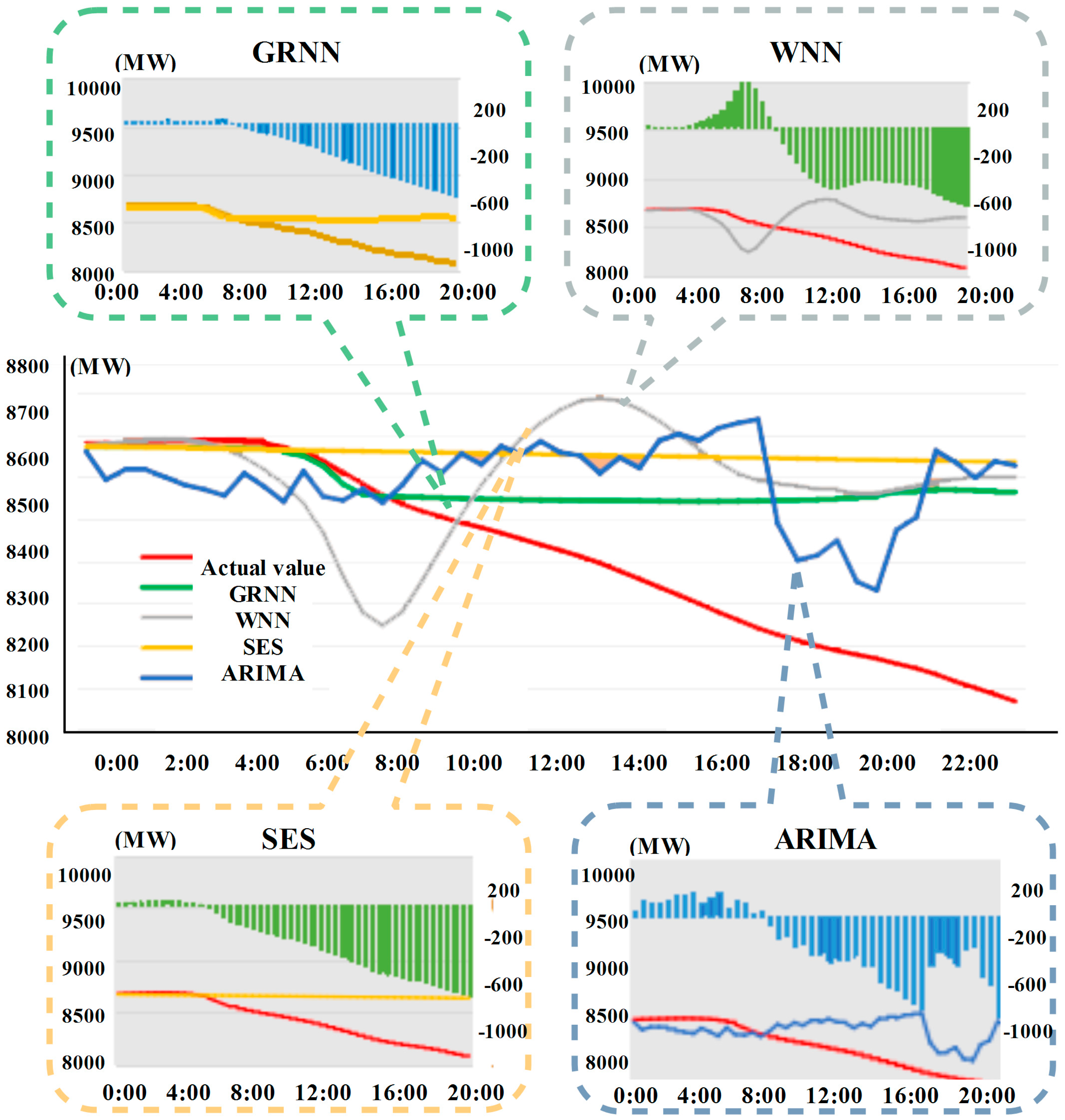
- (1)
- The speed to forecast the nonlinear time series data by using WNN is fast, with a better ability of generalization and a higher accuracy; however, the stability is weak.
- (2)
- The advantages of SES are the simple calculation, strong adaptability and stable forecasting results, but the ability to address nonlinear time series data is weak.
- (3)
- ARIMA performs well with a relatively higher accuracy when forecasting the electrical load data. However, as time goes by, the forecasting errors would gradually become larger and larger, which is only suitable for short-term forecasting.
- (4)
- On the whole, compared with other methods, GRNN can obtain a better and more stable forecasting result, as it deals with the non-linear data well and can fit and forecast the electrical load data well.
4.4. Comparative Analysis
- (1)
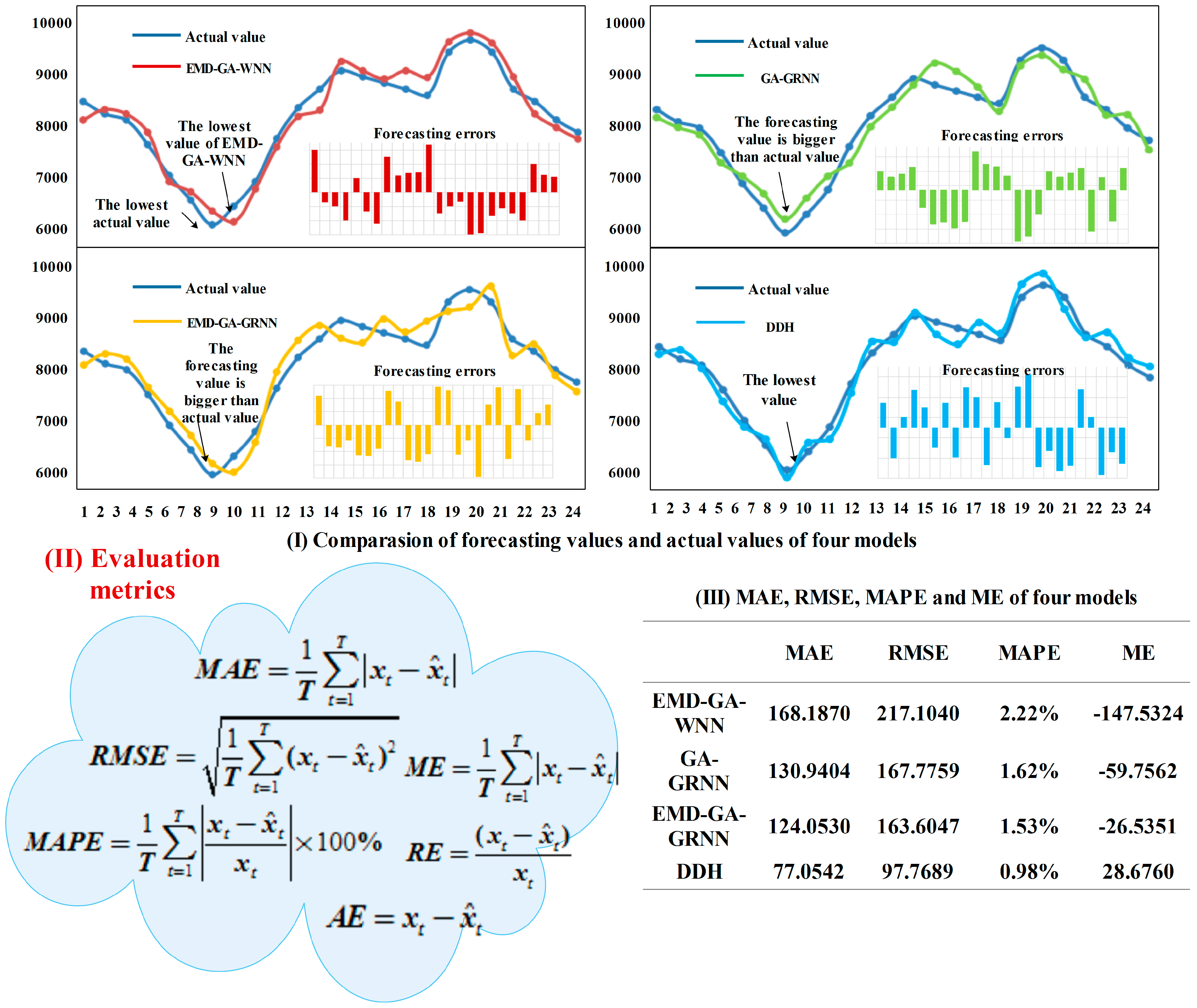
- From Figure 7, it can be seen that EMD-GA-WNN does not perform well when forecasting the electrical load data, and the relative errors of some parts even exceed 5%. This may be caused by the weak forecasting stability of WNN, and although GA can optimize its parameters, the effect to improve its stability is weak.
- (2)
- As for GA-GRNN and EMD-GA-GRNN, MAPEs are all within 5%, which indicates that the two forecasting models have better performance. In detail, the forecasting effect of EMD-GA-GRNN is much better than that of GA-GRNN, proving the function of EMD in improving the forecasting accuracy.
- (3)
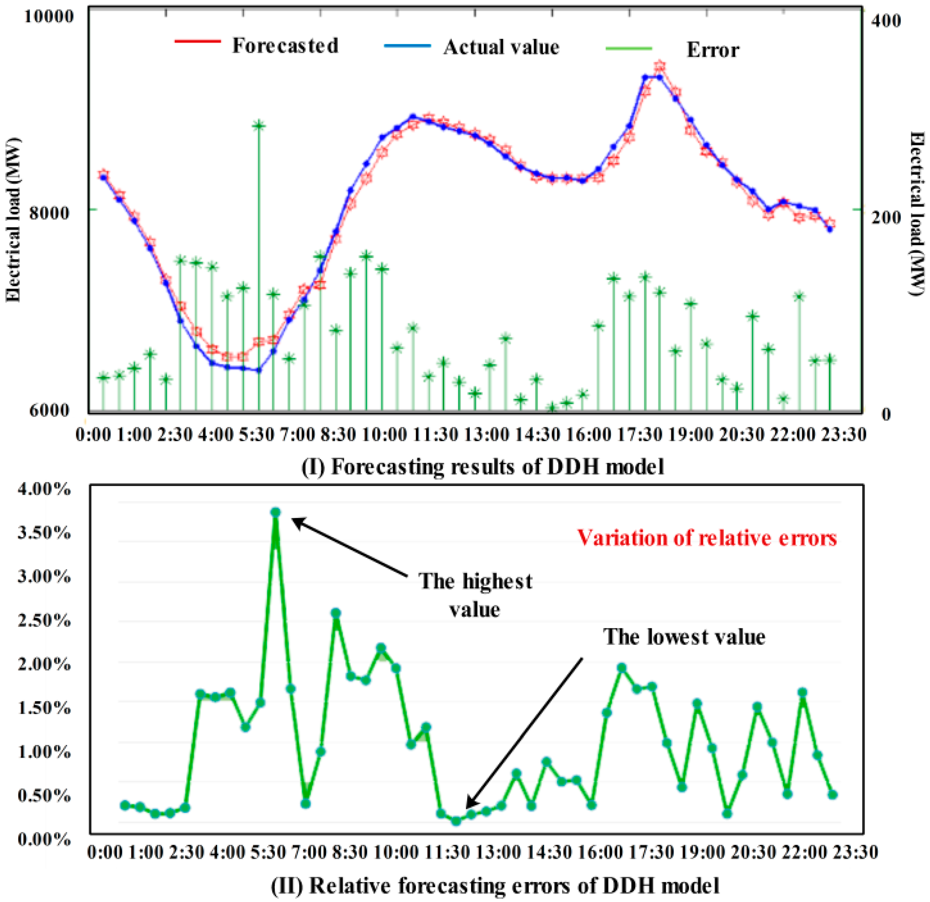
- The DDH model based on the data decomposition put forward in this paper can control the MAPE at 4%; thus, it can be known that it has a very strong fitting ability for non-linear data and forecasting ability for the electrical load time series. Both the simulation results and the forecasting process demonstrate that the proposed model can have a good performance when forecasting the non-linear time series data with periodicity, trend and randomness.
- (4)
- From the evaluation metrics in Figure 7, it can be known that the forecasting ability of GRNN is better than WNN, which is because that GRNN can deal well with the data such as electrical load time series; therefore, this paper also establishes the model based on GRNN. The proposed forecasting model EMD-GA-GRNN and EMD-GA-GRNN based on WNN and GRNN can improve the forecasting accuracy well. However, in comparison, GRNN is more suitable for the nonlinear time series data, and MAPEs of EMD-GA-WNN and EMD-GA-GRNN are 2.22% and 1.53%, respectively. Certainly, EMD can reduce the forecasting errors in some degree. Besides, MAPE decreases from 1.62% of GA-GRNN to 1.53% of EMD-GA-GRNN. However, DDH model can reduce MAPE within 1%.
4.5. Further Experiments
- (1)
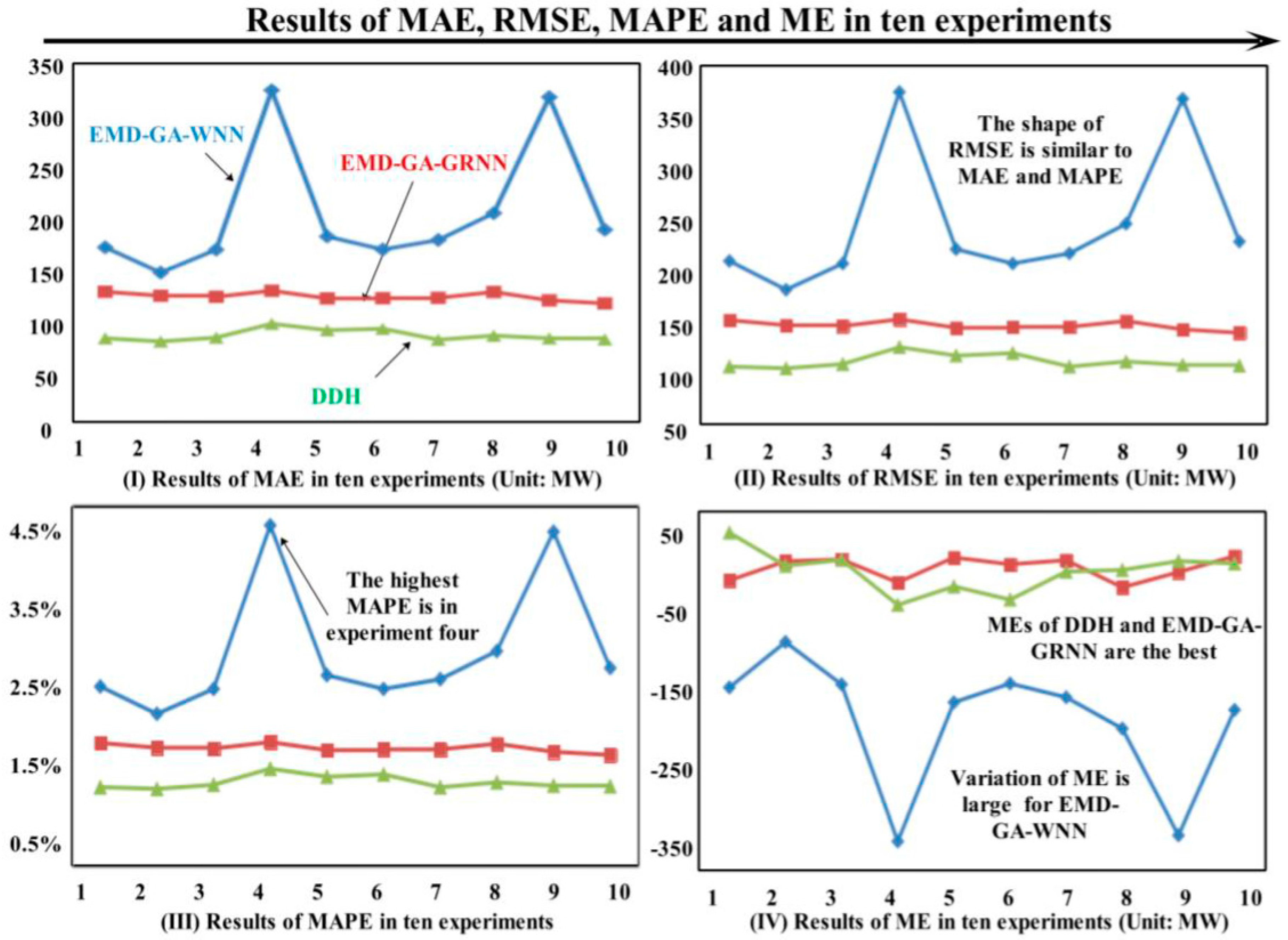
- As for the weekly analysis, it can be seen that the average MAPE of DDH in one week is 1.01%, which is lower than EMD-GA-WNN and EMD-GA-GRNN. About other indexes, including MAE, RMSE and ME, DDH all obtain the best forecasting results. When comparing the working days with weekends, the proposed hybrid model can both have a high forecasting accuracy, which proves the effectiveness of the model.
- (2)
- Table 5 shows the forecasting results of days in different seasons. Based on the comparison, it can be concluded that DDH is superior to the other two models with the values of MAPE 0.96%, 1.18%, 1.18% and 1.13% in spring, summer, autumn and winter, respectively. The results can validate that the proposed hybrid DDH model has a high degree of robustness and forecasting accuracy.
4.6. Discussion on Model Features
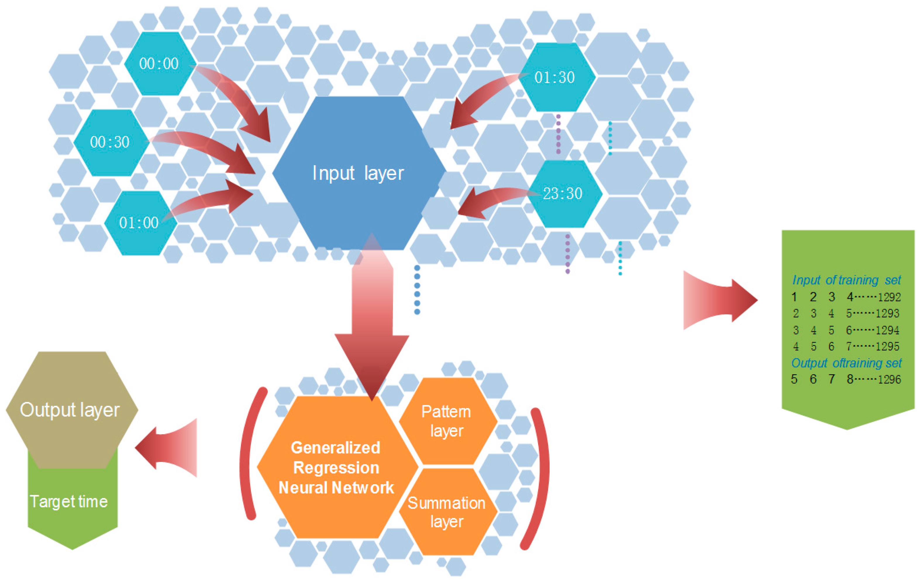
- It has a relatively low requirement for the sample size during the model building process, which can reduce the computing complexity;
- The human error is small. Compared with the back propagation neural network (BPNN), GRNN is different. During the training process, the historical samples will directly control the learning process without adjusting the connection weight of neurons. What is more, parameters like learning rate, training time and the type of transfer function, need to be adjusted. Accordingly, there is only one parameter in GRNN that needs to be set artificially, which is the smoothing factor;
- Strong self-learning ability and perfect nonlinear mapping ability. GRNN belongs to a branch of RBF neural networks with strong nonlinear mapping function. To apply GRNN in electrical load forecasting can better reflect the nonlinear mapping relationship;
- Fast learning rate. GRNN uses BP algorithm to modify the connection weight of the relative network, and applies the Gaussian function to realize the internal approximation function, which can help arrive at an efficient learning rate. The above features of GRNN play a pivotal role in performing the electrical load forecasting when the original data are fluctuating and non-linear.
- Self-adaptability. When solving problems, GA deals with the chromosome individuals through coding. During the process of evolution, GA will search the optimal individuals based on the fitness function. If the fitness value of chromosome is large, it indicates a stronger adaptability. It obeys the rules of survival of the fittest; meanwhile, it can keep the best state in a changing environment;
- Population search. The conventional methods usually search for single points, which is easily trapped into a local optimum if a multimodal distribution exists in the search space. However, GA can search from multiple starting points and evaluate several individuals at the same time, which makes it achieve a better global searching;
- Need for a small amount of information. GA only uses the fitness function to evaluate the individuals without referring to other information. It has a small dependence or limitation conditions to the problems, so it has a wider applicability;
- Heuristic random search. GA highlights the probability transformation instead of the certain transformation rule;
- Parallelism. On the one hand, it can search multiple individuals in the solution space; on the other hand, multiple computers can be applied to perform the evolution calculation to choose the best individuals until the computation ends. The above advantages make GA widely used in many fields, such as function optimization, production dispatching, data mining, forecasting for electrical load and so on.
5. Conclusions
Acknowledgments
Author Contributions
Conflicts of Interest
Abbreviations
| ANNs | Artificial neural networks |
| SVM | Support vector machine |
| EA | Evolution algorithms |
| ARIMA | Auto regressive integrated moving average |
| SOM | Self-organizing map |
| GRNN | Generalized regression neural network |
| EMD | Empirical mode decomposition |
| IMF | Intrinsic mode function |
| WNN | Wavelet neural network |
| SES | Secondary exponential smoothing |
| ANFIS | Adaptive network-based fuzzy inference system |
| RBFNN | Radial basis function neural network |
| HS-ARTMAP | Hyper-spherical ARTMAP network |
| RBF | Radial basis function |
| GA | Genetic algorithm |
| DDH | Data Decomposition Hybrid Model |
| MAE | Mean absolute error |
| RMSE | Root mean square error |
| MAPE | Mean absolute percentage error |
| ME | Mean error |
| AE | Absolute error |
| RE | Relative error |
| BPNN | Back propagation neural network |
| diff-SARIMA | Difference seasonal autoregressive integrated moving average |
| ART | Adaptive resonance theory |
| WT | Wavelet transform |
References
- Yang, Y.; Chen, Y.H.; Wang, Y.C.; Li, C.H.; Li, L. Modelling a combined method based on ANFIS and neural network improved by DE algorithm: A case study for short-term electricity demand forecasting. Appl. Soft Comput. 2015, 49, 663–675. [Google Scholar] [CrossRef]
- Li, S.; Goel, L.; Wang, P. An ensemble approach for short-term load forecasting by extreme learning machine. Appl. Energy 2016, 170, 22–29. [Google Scholar] [CrossRef]
- Takeda, H.; Tamura, Y.; Sato, S. Using the ensemble Kalman filter for electricity load forecasting and analysis. Energy 2016, 104, 184–198. [Google Scholar] [CrossRef]
- Xiao, L.Y.; Wang, J.Z.; Hou, R.; Wu, J. A combined model based on data pre-analysis and weight coefficients optimization for electrical load forecasting. Energy 2015, 82, 524–549. [Google Scholar] [CrossRef]
- Ren, Y.; Suganthan, P.N.; Srikanth, N.; Amaratunga, G. Random vector functional link network for short-term electricity load demand forecasting. Inf. Sci. 2016, 1, 1078–1093. [Google Scholar] [CrossRef]
- Xiao, L.Y.; Shao, W.; Liang, T.L.; Wang, C. A combined model based on multiple seasonal patterns and modified firefly algorithm for electrical load forecasting. Appl. Energy 2016, 167, 135–153. [Google Scholar] [CrossRef]
- Xiao, L.Y.; Shao, W.; Wang, C.; Zhang, K.Q.; Lu, H.Y. Research and application of a hybrid model based on multi-objective optimization for electrical load forecasting. Appl. Energy 2016, 180, 213–233. [Google Scholar] [CrossRef]
- Jiang, P.; Ma, X.J. A hybrid forecasting approach applied in the electrical power system based on data preprocessing, optimization and artificial intelligence algorithms. Appl. Math. Model. 2016, 40, 10631–10649. [Google Scholar] [CrossRef]
- Azadeh, A.; Ghaderi, S.F.; Sohrabkhani, S. A simulated-based neural network algorithm for forecasting electrical energy consumption in Iran. Energy Policy 2008, 36, 37–44. [Google Scholar] [CrossRef]
- Chang, P.C.; Fan, C.Y.; Lin, J.J. Monthly electricity demand forecasting based on a weighted evolving fuzzy neural network approach. Electr. Power Syst. Res. 2011, 33, 17–27. [Google Scholar] [CrossRef]
- Wang, J.Z.; Chi, D.Z.; Wu, J.; Lu, H.Y. Chaotic time serious method combined with particle swarm optimization and trend adjustment for electricity demand forecasting. Expert Syst. Appl. 2011, 38, 19–29. [Google Scholar] [CrossRef]
- Ghanbari, A.; Kazami, S.M.; Mehmanpazir, F.; Nakhostin, M.M. A cooperative ant colony optimization-genetic algorithm approach for construction of energy demand forecasting knowledge-based expert systems. Knowl. Based Syst. 2013, 39, 194–206. [Google Scholar] [CrossRef]
- Zhao, H.R.; Guo, S. An optimized grey model for annual power load forecasting. Energy 2016, 107, 272–286. [Google Scholar] [CrossRef]
- Zeng, B.; Li, C. Forecasting the natural gas demand in China using a self-adapting intelligent grey model. Energy 2016, 112, 810–825. [Google Scholar] [CrossRef]
- Kavaklioglu, K. Modeling and prediction of Turkeys electricity consumption using Support Vector Regression. Appl. Energy 2011, 88, 68–75. [Google Scholar] [CrossRef]
- Wang, J.Z.; Zhu, W.J.; Zhang, W.Y.; Sun, D.H. A trend fixed on firstly and seasonal adjustment model combined with the SVR for short-term forecasting of electricity demand. Energy Policy 2009, 37, 1–9. [Google Scholar] [CrossRef]
- Kucukali, S.; Baris, K. Turkeys shorts-term gross annual electricity demand forecast by fuzzy logic approach. Energy Policy 2010, 38, 38–45. [Google Scholar] [CrossRef]
- Nguyen, H.T.; Nabney, I.T. Short-term electricity demand and gas price forecasts using wavelet transforms and adaptive models. Energy 2010, 35, 13–21. [Google Scholar] [CrossRef]
- Park, D.C.; Sharkawi, M.A.; Marks, R.J. Electric load forecasting using a neural network. IEEE Trans. Power Syst. 1991, 6, 442–449. [Google Scholar] [CrossRef]
- Wang, J.Z.; Liu, F.; Song, Y.L.; Zhao, J. A novel model: Dynamic choice artificial neural network (DCANN) for an electricity price forecasting system. Appl. Soft Comput. 2016, 48, 281–297. [Google Scholar] [CrossRef]
- Yu, F.; Xu, X.Z. A short-term load forecasting model of natural gas based on optimized genetic algorithm and improved BP neural network. Appl. Energy 2014, 134, 102–113. [Google Scholar] [CrossRef]
- Hernandez, L.; Baladron, C.; Aguiar, J.M. Short-term load forecasting for microgrids based on artificial neural networks. Energies 2013, 6, 1385–1408. [Google Scholar] [CrossRef]
- Pandian, S.C.; Duraiswamy, K.D.; Rajan, C.C.; Kanagaraj, N. Fuzzy approach for short term load forecasting. Electr. Power Syst. Res. 2006, 76, 541–548. [Google Scholar] [CrossRef]
- Pai, P.F. Hybrid ellipsoidal fuzzy systems in forecasting regional electricity loads. Energy Convers. Manag. 2006, 47, 2283–2289. [Google Scholar] [CrossRef]
- Liu, L.W.; Zong, H.J.; Zhao, E.D.; Chen, C.X.; Wang, J.Z. Can China realize its carbon emission reduction goal in 2020: From the perspective of thermal power development. Appl. Energy 2014, 124, 199–212. [Google Scholar] [CrossRef]
- Xiao, L.; Wang, J.Z.; Dong, Y.; Wu, J. Combined forecasting models for wind energy forecasting: A case stud in China. Renew. Sustain. Energy Rev. 2015, 44, 271–288. [Google Scholar] [CrossRef]
- Wang, J.J.; Wang, J.Z.; Li, Y.N.; Zhu, S.L.; Zhao, J. Techniques of applying wavelet de-noising into a combined model for short-term load forecasting. Int. J. Electr. Power 2014, 62, 816–824. [Google Scholar] [CrossRef]
- Azimi, R.; Ghofrani, M.; Ghayekhloo, M. A hybrid wind power forecasting model based on data mining and wavelets analysis. Energy Convers. Manag. 2016, 127, 208–225. [Google Scholar] [CrossRef]
- Khashei, M.; Bijari, M. An artificial neural network model for time series forecasting. Expert Syst. 2010, 37, 479–489. [Google Scholar] [CrossRef]
- Shukur, O.B.; Lee, M.H. Daily wind speed forecasting though hybrid KF-ANN model based on ARIMA. Renew. Energy 2015, 76, 637–647. [Google Scholar] [CrossRef]
- Niu, D.; Shi, H.; Wu, D.D. Short-term load forecasting using bayesian neural networks learned by hybrid Monte Carlo algorithm. Appl. Soft Comput. 2012, 12, 1822–1827. [Google Scholar] [CrossRef]
- Lu, C.J.; Wang, Y.W. Combining independent component analysis and growing hierarchical self-organizing maps with support vector regression in product demand forecasting. Int. J. Prod. Econ. 2010, 128, 603–613. [Google Scholar] [CrossRef]
- Okumus, I.; Dinler, A. Current status of wind energy forecasting and a hybrid method for hourly predictions. Energy Convers. Manag. 2016, 123, 362–371. [Google Scholar] [CrossRef]
- Che, J.; Wang, J. Short-term electricity prices forecasting based on support vector regression and auto-regressive integrated moving average modeling. Energy Convers. Manag. 2010, 51, 1911–1917. [Google Scholar] [CrossRef]
- Meng, A.B.; Ge, J.F.; Yin, H.; Chen, S.Z. Wind speed forecasting based on wavelet packet decomposition and artificial neural networks trained by crisscross optimization algorithm. Energy Convers. Manag. 2016, 114, 75–88. [Google Scholar] [CrossRef]
- Elvira, L.N. Annual Electrical Peak Load Forecasting Methods with Measures of Prediction Error 2002. Ph.D. Thesis, Arizona State University, Tempe, AZ, USA, 2002. [Google Scholar]
- Wang, J.Z.; Ma, X.L.; Wu, J.; Dong, Y. Optimization models based on GM (1,1) and seasonal fluctuation for electricity demand forecasting. Int. J. Electr. Power 2012, 43, 109–117. [Google Scholar] [CrossRef]
- Guo, Z.H.; Wu, J.; Lu, H.Y.; Wang, J.Z. A case study on a hybrid wind speed forecasting method using BP neural network. Knowl. Based Syst. 2011, 2, 1048–1056. [Google Scholar] [CrossRef]
- Peng, L.L.; Fan, G.F.; Huang, M.L.; Hong, W.C. Hybridizing DEMD and quantum PSO with SVR in electric load forecasting. Energies 2016, 9. [Google Scholar] [CrossRef]
- Fan, G.F.; Peng, L.L.; Hong, W.C.; Sun, F. Electric load forecasting by the SVR model with differential empirical mode decomposition and auto regression. Neurocomputing 2016, 173, 958–970. [Google Scholar] [CrossRef]
- Liu, H.; Tian, H.Q.; Liang, X.F.; Li, Y.F. New wind speed forecasting approaches using fast ensemble empirical model decomposition, genetic algorithm, mind evolutionary algorithm and artificial neural networks. Renew. Energy 2015, 83, 1066–1075. [Google Scholar] [CrossRef]
- Niu, D.X.; Cao, S.H.; Zhao, L.; Zhang, W.W. Methods for Electrical Load Forecasting and Application; China Electric Power Press: Beijing, China, 1998. [Google Scholar]
- Liu, L.; Wang, Q.R.; Wang, J.Z.; Liu, M. A rolling grey model optimized by particle swarm optimization in economic prediction. Comput. Intell. 2014, 32, 391–419. [Google Scholar] [CrossRef]
- Yuan, C.; Wang, J.Z.; Tang, Y.; Yang, Y.C. An efficient approach for electrical load forecasting using distributed ART (adaptive resonance theory) & HS-ARTMAP (Hyper-spherical ARTMAP network) neural network. Energy 2011, 36, 1340–1350. [Google Scholar]
- Hooshmand, R.A.; Amooshahi, H.; Parastegari, M. A hybrid intelligent algorithm based short-term load forecasting approach. Int. J. Electr. Power 2013, 45, 313–324. [Google Scholar] [CrossRef]


| Name of Metrics | Equation | No. | Name of Metrics | Equation | No. |
|---|---|---|---|---|---|
| MAE | (35) | ME | (38) | ||
| RMSE | (36) | AE | (39) | ||
| MAPE | (37) | RE | (40) |
| Time | Actual Value | Forecasting Output of the Model | Time | Actual Value | Forecasting Output of the Model | ||||||
|---|---|---|---|---|---|---|---|---|---|---|---|
| EMD-GA-WNN | GA-GRNN | EMD-GA-GRNN | DDH | EMD-GA-WNN | GA-GRNN | EMD-GA-GRNN | DDH | ||||
| 0:00 | 8314.34 | 8316.79 | 8485.70 | 8448.82 | 8297.61 | 12:00 | 8731.01 | 8911.29 | 8740.80 | 8749.89 | 8719.90 |
| 0:30 | 8097.56 | 8120.24 | 8324.54 | 8277.18 | 8082.89 | 12:30 | 8649.94 | 8869.53 | 8629.02 | 8653.62 | 8667.12 |
| 1:00 | 7881.03 | 7928.45 | 8120.26 | 8077.17 | 7873.46 | 13:00 | 8520.88 | 8820.83 | 8534.06 | 8544.21 | 8572.19 |
| 1:30 | 7613.53 | 7687.64 | 7880.49 | 7856.92 | 7621.62 | 13:30 | 8419.95 | 8746.33 | 8436.37 | 8418.62 | 8403.67 |
| 2:00 | 7265.94 | 7330.03 | 7586.18 | 7558.97 | 7253.44 | 14:00 | 8359.06 | 8668.88 | 8332.43 | 8324.83 | 8296.61 |
| 2:30 | 6884.16 | 7067.63 | 7116.65 | 7134.47 | 6993.73 | 14:30 | 8304.55 | 8570.31 | 8261.18 | 8263.58 | 8263.13 |
| 3:00 | 6638.55 | 6870.98 | 6725.93 | 6750.43 | 6741.38 | 15:00 | 8312.49 | 8529.19 | 8219.80 | 8205.82 | 8269.39 |
| 3:30 | 6464.02 | 6743.91 | 6519.60 | 6508.65 | 6567.98 | 15:30 | 8285.25 | 8513.52 | 8219.06 | 8196.43 | 8268.39 |
| 4:00 | 6421.67 | 6707.56 | 6392.63 | 6404.61 | 6497.16 | 16:00 | 8401.56 | 8545.67 | 8210.85 | 8185.83 | 8287.56 |
| 4:30 | 6412.23 | 6724.73 | 6419.99 | 6451.49 | 6507.20 | 16:30 | 8616.59 | 8660.40 | 8297.24 | 8257.93 | 8451.27 |
| 5:00 | 6394.72 | 6873.82 | 6536.38 | 6556.23 | 6641.75 | 17:00 | 8829.22 | 8806.80 | 8600.25 | 8503.72 | 8683.46 |
| 5:30 | 6582.09 | 7033.42 | 6598.89 | 6605.74 | 6691.06 | 17:30 | 9308.85 | 9216.90 | 9000.54 | 8890.66 | 9152.10 |
| 6:00 | 6899.25 | 7399.88 | 6802.04 | 6814.45 | 6914.60 | 18:00 | 9307.55 | 9429.90 | 9249.77 | 9200.67 | 9398.89 |
| 6:30 | 7093.06 | 7642.45 | 7200.95 | 7193.05 | 7155.01 | 18:30 | 9106.91 | 9271.13 | 9328.58 | 9330.35 | 9145.80 |
| 7:00 | 7395.69 | 7715.40 | 7589.45 | 7524.90 | 7203.21 | 19:00 | 8893.08 | 8987.73 | 9292.04 | 9240.84 | 8762.06 |
| 7:30 | 7783.28 | 7973.56 | 7850.94 | 7754.65 | 7642.06 | 19:30 | 8641.32 | 8747.35 | 9042.83 | 8970.91 | 8562.08 |
| 8:00 | 8193.10 | 8145.44 | 8135.61 | 8026.69 | 8048.81 | 20:00 | 8437.27 | 8565.72 | 8596.66 | 8541.77 | 8445.35 |
| 8:30 | 8454.25 | 8325.99 | 8475.43 | 8493.17 | 8270.93 | 20:30 | 8297.38 | 8389.37 | 8407.47 | 8394.00 | 8249.05 |
| 9:00 | 8710.86 | 8616.62 | 8718.43 | 8606.26 | 8544.31 | 21:00 | 8174.13 | 8189.12 | 8278.29 | 8260.20 | 8057.12 |
| 9:30 | 8806.93 | 8824.25 | 8975.41 | 8860.02 | 8722.24 | 21:30 | 8004.14 | 7998.97 | 8129.02 | 8116.55 | 7925.10 |
| 10:00 | 8920.64 | 8984.50 | 8994.28 | 8924.99 | 8815.63 | 22:00 | 8077.99 | 8098.08 | 7964.69 | 7949.84 | 8050.27 |
| 10:30 | 8872.57 | 9023.17 | 9034.39 | 8910.56 | 8863.76 | 22:30 | 8033.84 | 7965.71 | 7977.29 | 7939.60 | 7904.37 |
| 11:00 | 8816.19 | 8981.31 | 8953.15 | 8840.24 | 8815.61 | 23:00 | 7989.55 | 7951.66 | 8016.42 | 7970.00 | 7923.18 |
| 11:30 | 8777.05 | 8946.75 | 8844.91 | 8810.79 | 8769.22 | 23:30 | 7803.73 | 7841.56 | 8020.16 | 7972.34 | 7829.81 |
| No. | EMD-GA-WNN | EMD-GA-GRNN | DDH | |||||||||
|---|---|---|---|---|---|---|---|---|---|---|---|---|
| MAE | RMSE | MAPE | ME | MAE | RMSE | MAPE | ME | MAE | RMSE | MAPE | ME | |
| 1 | 168.9702 | 218.9832 | 0.0223 | −150.3171 | 124.0530 | 163.6047 | 0.0153 | −26.5351 | 77.0542 | 97.7687 | 0.0098 | 28.6760 |
| 2 | 143.4750 | 187.9665 | 0.0189 | −97.7305 | 120.0837 | 160.1870 | 0.0147 | −4.4056 | 73.8617 | 90.7383 | 0.0096 | −9.6550 |
| 3 | 166.6531 | 215.6456 | 0.0220 | −146.7813 | 119.0237 | 161.9871 | 0.0146 | −2.3599 | 77.7576 | 96.1427 | 0.0101 | −2.7978 |
| 4 | 327.7693 | 366.7733 | 0.0423 | −327.7693 | 125.1301 | 160.2820 | 0.0154 | −28.9499 | 91.7547 | 110.8149 | 0.0121 | −54.7912 |
| 5 | 179.9683 | 231.0331 | 0.0237 | −167.4704 | 117.3492 | 158.6897 | 0.0144 | −0.0239 | 85.2639 | 101.5193 | 0.0111 | −33.4767 |
| 6 | 166.7894 | 215.3270 | 0.0220 | −145.6936 | 117.6313 | 157.8023 | 0.0145 | −7.9405 | 86.7251 | 105.4555 | 0.0114 | −48.7363 |
| 7 | 176.4214 | 228.1589 | 0.0232 | −161.6078 | 117.9699 | 158.3187 | 0.0145 | −3.1824 | 75.6047 | 90.9116 | 0.0098 | −16.3685 |
| 8 | 203.5435 | 250.7716 | 0.0267 | −197.7634 | 123.8518 | 163.8211 | 0.0152 | −34.5862 | 79.7625 | 96.8084 | 0.0104 | −14.4799 |
| 9 | 320.8268 | 358.9548 | 0.0415 | −320.8268 | 115.4209 | 157.6318 | 0.0142 | −16.9704 | 77.0379 | 94.9811 | 0.0100 | −4.2135 |
| 10 | 186.7493 | 239.4212 | 0.0246 | −176.1809 | 112.3399 | 155.0562 | 0.0138 | 1.6029 | 75.9955 | 93.4155 | 0.0099 | −6.9212 |
| Mean | 204.1166 | 251.3035 | 0.0267 | −189.2141 | 119.2854 | 159.7381 | 0.0147 | −12.3351 | 80.0818 | 97.8556 | 0.0104 | −16.2764 |
| Monday | Tuesday | Wednesday | Thursday | Friday | Saturday | Sunday | Week | |
|---|---|---|---|---|---|---|---|---|
| EMD-GA-WNN | ||||||||
| MAE | 117.6839 | 129.4867 | 142.1135 | 279.4283 | 225.6017 | 118.0649 | 206.1598 | 174.0770 |
| RMSE | 288.4620 | 237.0900 | 218.0418 | 211.3369 | 202.1987 | 245.0624 | 289.4222 | 241.6591 |
| MAPE | 0.0249 | 0.0286 | 0.0273 | 0.0263 | 0.0275 | 0.0219 | 0.0226 | 0.0256 |
| ME | −129.1364 | −18.7732 | −130.2645 | −88.3712 | −32.1989 | −60.3024 | −115.4213 | −82.0668 |
| EMD-GA-GRNN | ||||||||
| MAE | 117.6850 | 126.4213 | 110.0889 | 112.1325 | 129.0178 | 157.3144 | 138.0976 | 127.2511 |
| RMSE | 141.7699 | 168.3712 | 155.2626 | 148.0987 | 161.5546 | 132.1019 | 168.3174 | 153.6395 |
| MAPE | 0.0144 | 0.0137 | 0.0149 | 0.0155 | 0.0158 | 0.0159 | 0.0142 | 0.0149 |
| ME | −98.6273 | −87.0125 | −110.2455 | −136.4188 | −65.231 | −21.0987 | −33.4685 | −78.8718 |
| DDH | ||||||||
| MAE | 76.4219 | 88.1348 | 76.1653 | 79.0187 | 84.315 | 69.1083 | 70.4245 | 77.6555 |
| RMSE | 97.6681 | 102.4269 | 99.8349 | 105.1917 | 112.3416 | 108.1947 | 98.1032 | 103.3944 |
| MAPE | 0.0101 | 0.0094 | 0.0112 | 0.0095 | 0.0098 | 0.0106 | 0.0103 | 0.0101 |
| ME | −13.0719 | −2.0715 | −4.3728 | 18.1605 | 12.1004 | −34.5671 | −10.0628 | −4.8407 |
| Evaluation Index | EMD-GA-WNN | EMD-GA-GRNN | DDH | Evaluation Index | EMD-GA-WNN | EMD-GA-GRNN | DDH |
|---|---|---|---|---|---|---|---|
| Spring | Summer | ||||||
| MAE | 119.4287 | 117.0216 | 76.0138 | MAE | 137.0345 | 108.417 | 60.1837 |
| RMSE | 292.0655 | 140.3726 | 97.0138 | RMSE | 213.0418 | 156.1783 | 94.1296 |
| MAPE | 0.0231 | 0.0158 | 0.0096 | MAPE | 0.0274 | 0.0162 | 0.0118 |
| ME | −112.0659 | −78.4257 | −16.1076 | ME | −97.3125 | −52.1035 | −20.0244 |
| Autumn | Winter | ||||||
| MAE | 125.0638 | 100.0246 | 78.1025 | MAE | 112.0605 | 100.4629 | 73.1068 |
| RMSE | 213.1294 | 148.7329 | 89.4237 | RMSE | 200.0217 | 158.0376 | 971136 |
| MAPE | 0.0219 | 0.0143 | 0.0118 | MAPE | 0.0212 | 0.0158 | 0.0113 |
| ME | −101.0137 | −25.4269 | −11.0036 | ME | −94.1346 | −36.0599 | −11.0217 |
| Model | Period | MAPE (%) | Ref. |
|---|---|---|---|
| Combined model based on BPNN, ANFIS and diff-SARIMA | Data from May to June 2011 | 1.654 | [1] |
| Combined model based on BPNN, RBFNN,GRNN and GA-BPNN | Data from February 2006 to February 2009 | 1.236 | [4] |
| HS-ARTMAP network | Data in the head days in January from 1999 to 2009 | 1.900 | [44] |
| Hybrid model based on WT, ANN and ANFIS | Data from 12 July to 31 July 2004 | 1.603 | [45] |
| The proposed DDH | Data from April to June 2011 | 1.010 | / |
| Model | Nonlinear Mapping Ability | Set parameters Artificially | Generalization | Robustness | Fault Tolerance | Structural Interpretability | Convergence Ability | Sample Size |
|---|---|---|---|---|---|---|---|---|
| Grey model | Middle | Middle | Weak | Weak | Weak | Good interpretability for internal structure | ---- | Large |
| Regression model | Weak | Large | Middle | Weak | Weak | Good interpretability for internal structure | ---- | Large |
| Back Propagation (BP) model | Strong | Large | Middle | Middle | Weak | No structural interpretability | Weak | Large |
| GRNN model | Strong | Only smoothing factor parameter | Strong | Strong | Strong | No structural interpretability | Strong | Low requirement |
© 2016 by the authors; licensee MDPI, Basel, Switzerland. This article is an open access article distributed under the terms and conditions of the Creative Commons Attribution (CC-BY) license (http://creativecommons.org/licenses/by/4.0/).
Share and Cite
Dong, Y.; Ma, X.; Ma, C.; Wang, J. Research and Application of a Hybrid Forecasting Model Based on Data Decomposition for Electrical Load Forecasting. Energies 2016, 9, 1050. https://doi.org/10.3390/en9121050
Dong Y, Ma X, Ma C, Wang J. Research and Application of a Hybrid Forecasting Model Based on Data Decomposition for Electrical Load Forecasting. Energies. 2016; 9(12):1050. https://doi.org/10.3390/en9121050
Chicago/Turabian StyleDong, Yuqi, Xuejiao Ma, Chenchen Ma, and Jianzhou Wang. 2016. "Research and Application of a Hybrid Forecasting Model Based on Data Decomposition for Electrical Load Forecasting" Energies 9, no. 12: 1050. https://doi.org/10.3390/en9121050
APA StyleDong, Y., Ma, X., Ma, C., & Wang, J. (2016). Research and Application of a Hybrid Forecasting Model Based on Data Decomposition for Electrical Load Forecasting. Energies, 9(12), 1050. https://doi.org/10.3390/en9121050