
Mitigation of the Impact of High Plug-in Electric Vehicle Penetration on Residential Distribution Grid Using Smart Charging Strategies

Abstract
:1. Introduction
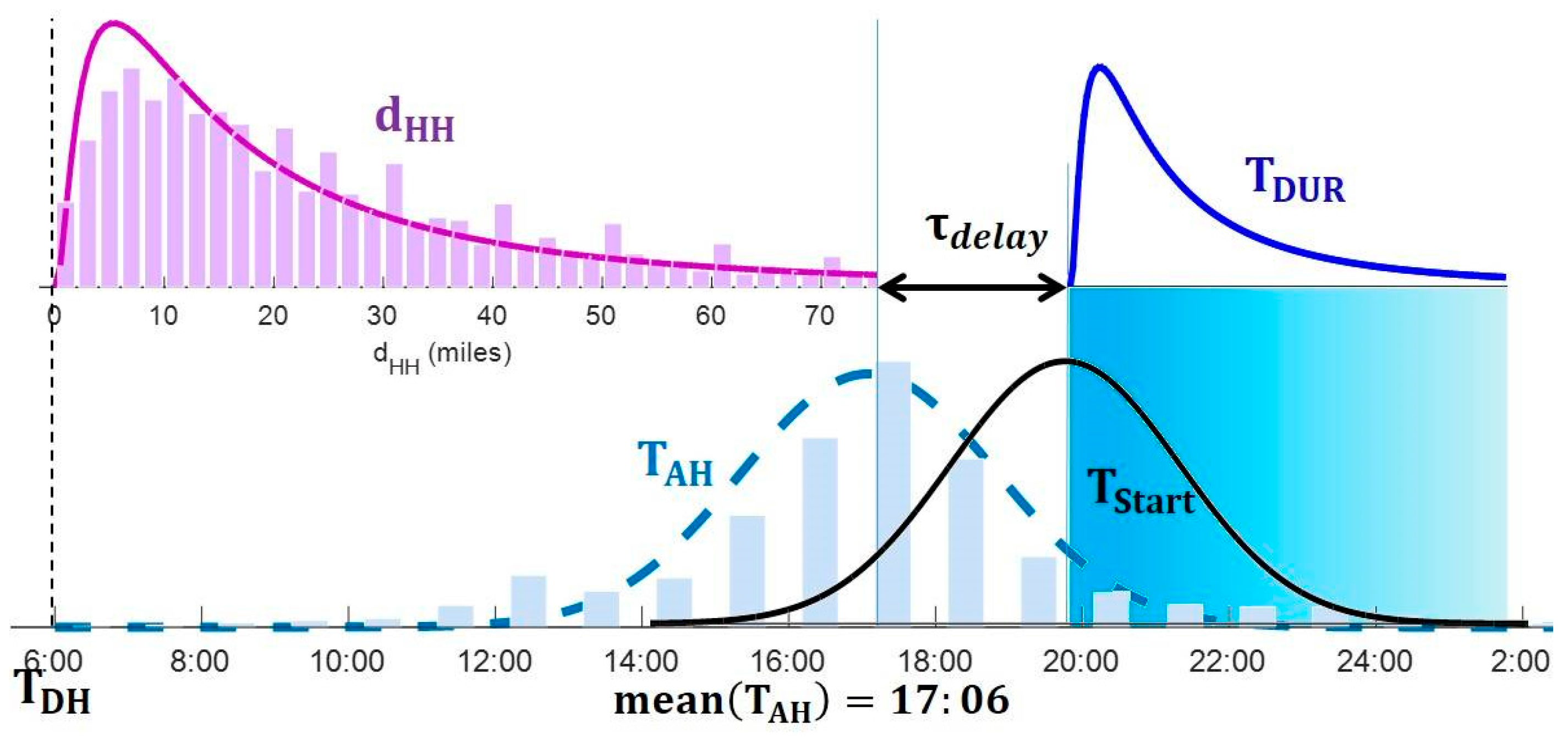
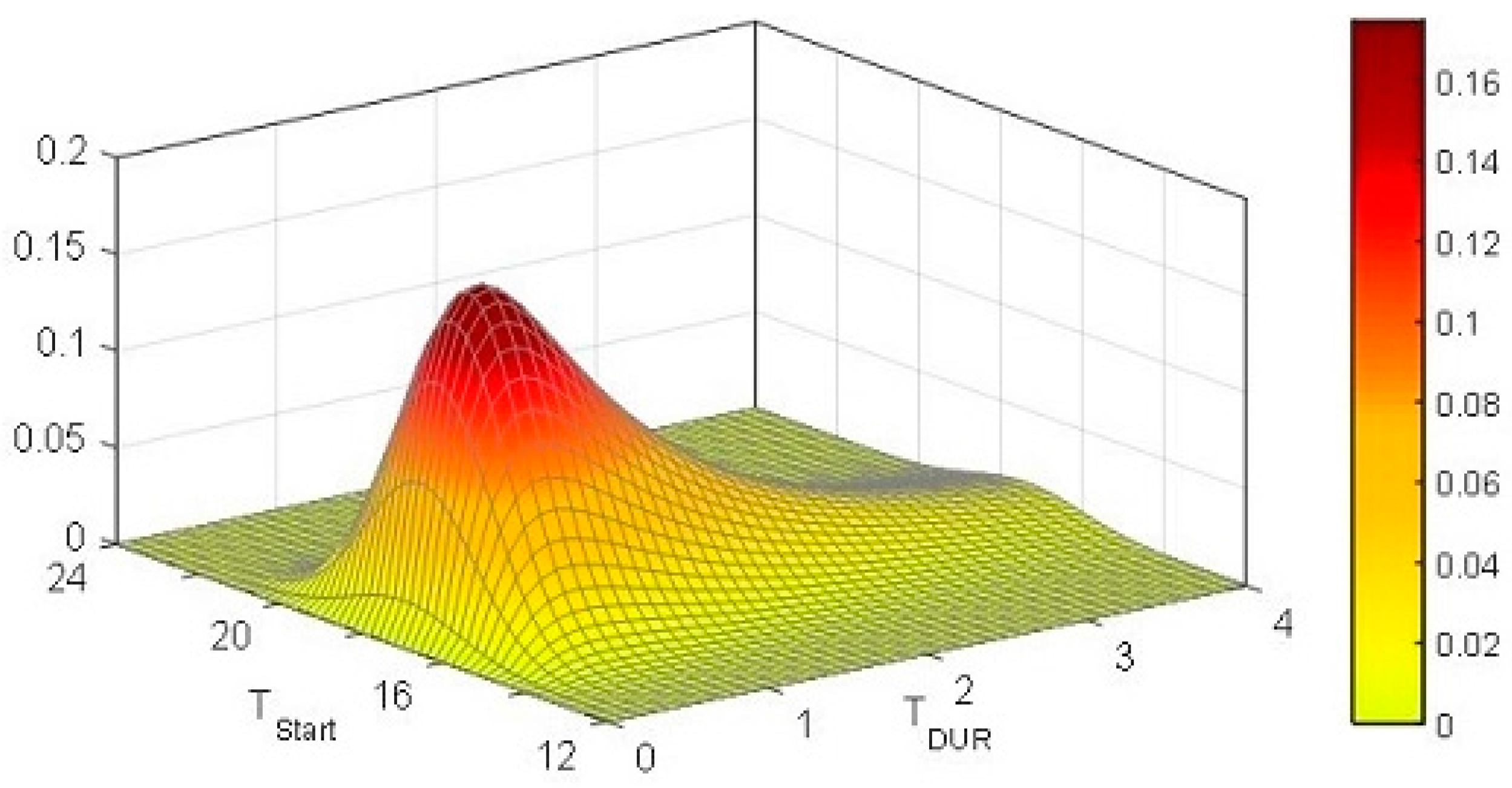
2. Stochastic Modeling of Plug-in Electric Vehicle Fleet Charging
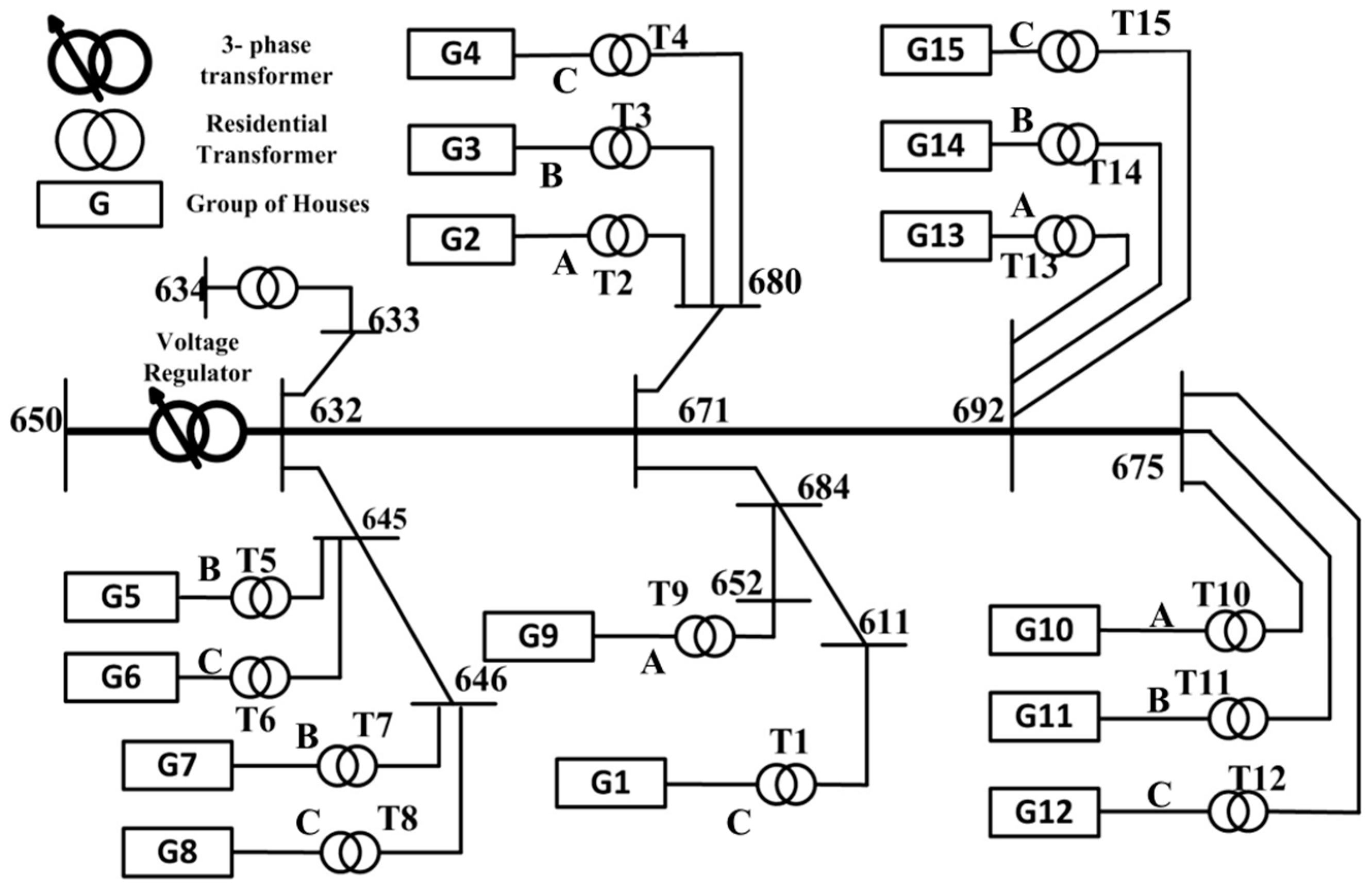
3. Residential Distribution Grid for Impact Study
3.1. Residential Baseline Load Modeling
3.2. Power Demand at Transformer
4. Impact of Plug-in Electric Vehicle Charging on Residential Distribution Grid
4.1. Load Surge
4.2. Voltage Deviation
4.3. Impact on Local Transformer Aging
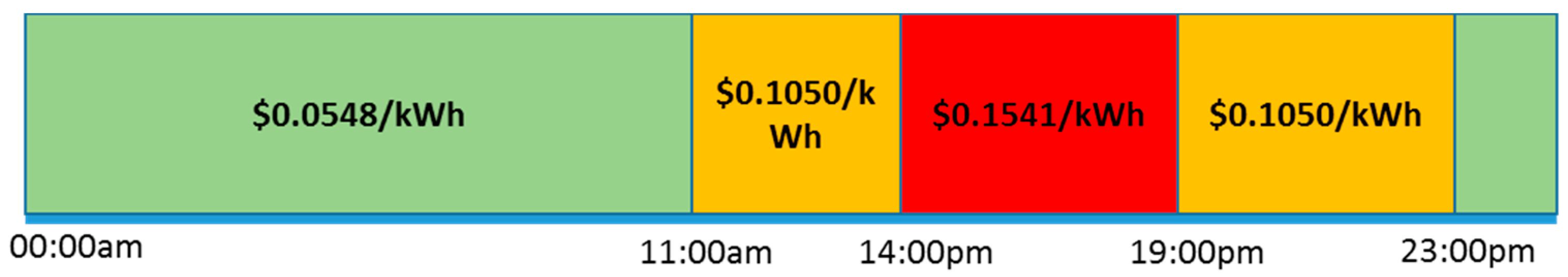
5. Managed Plug-in Electric Vehicle Charging with Smart Charging Strategies
6. Simulation Results
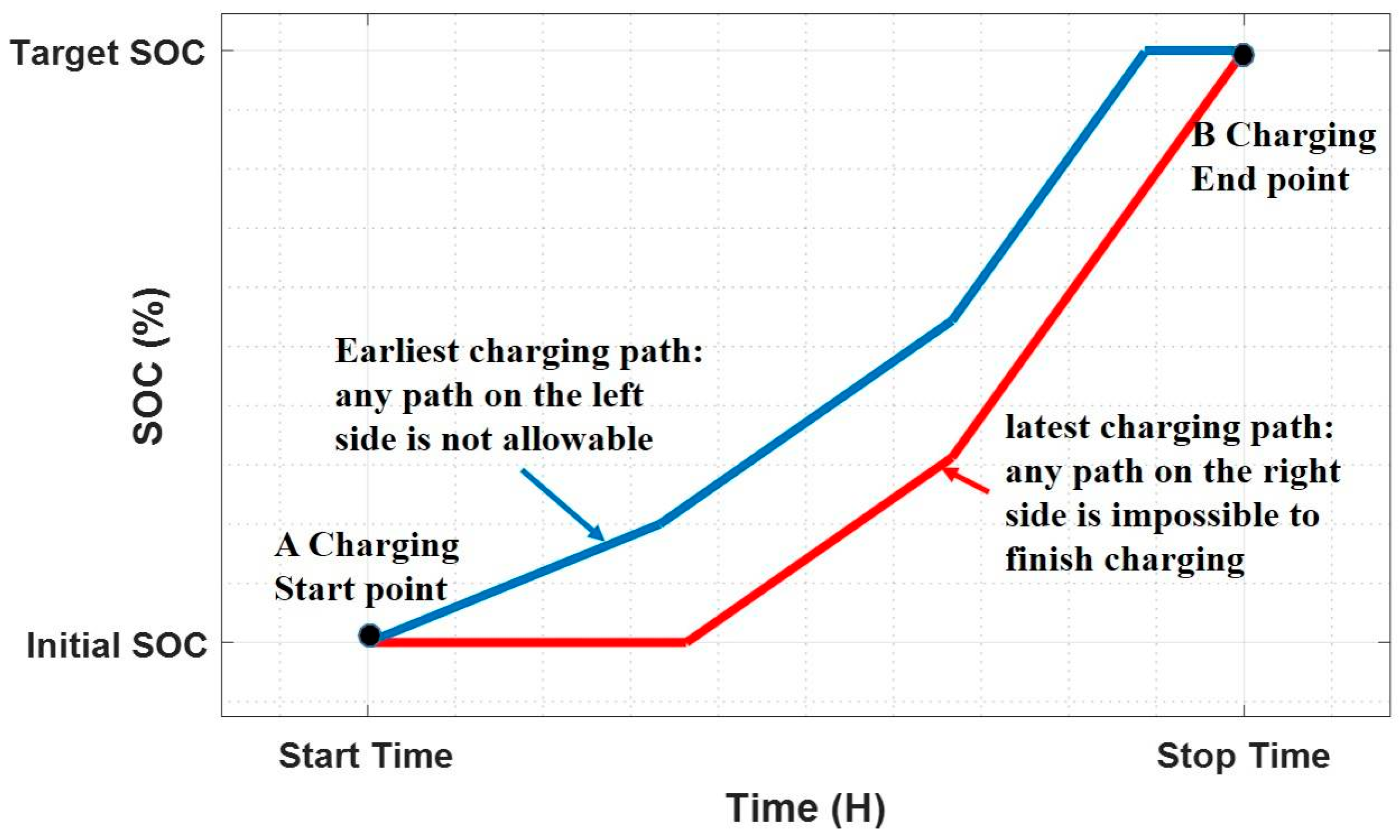
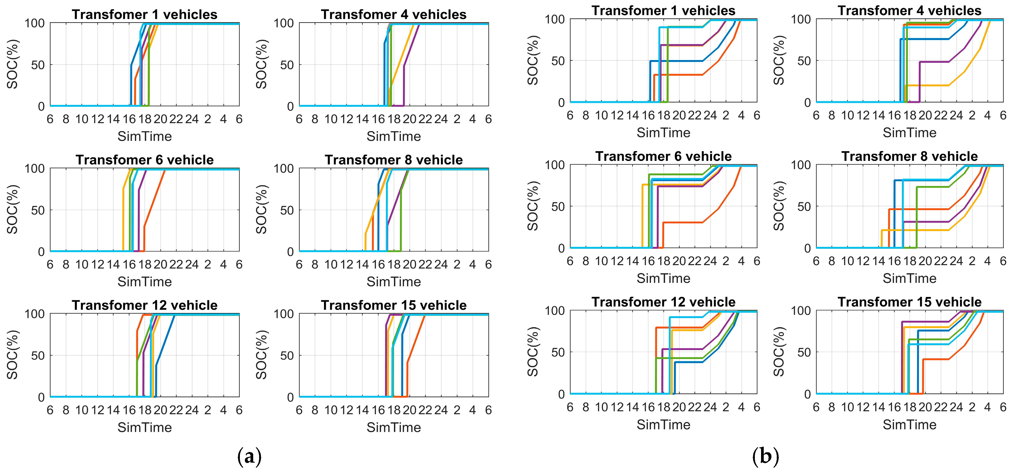
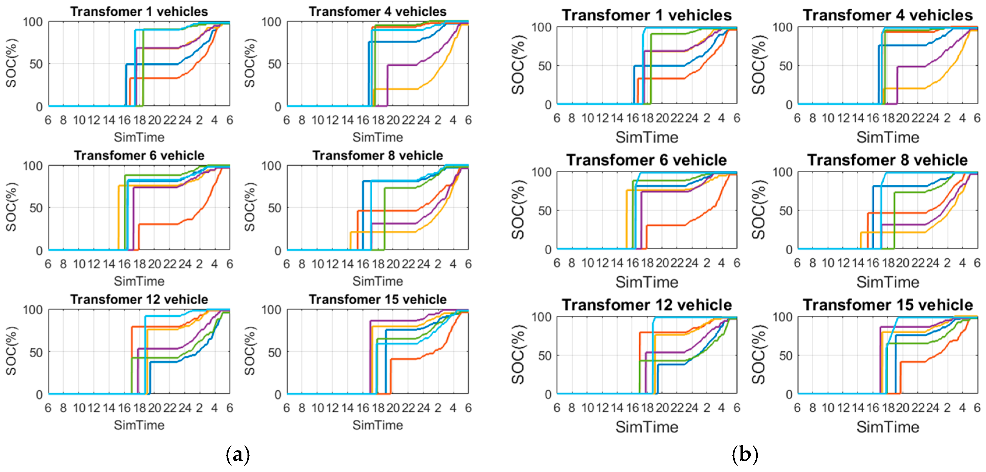
6.1. Charging Path
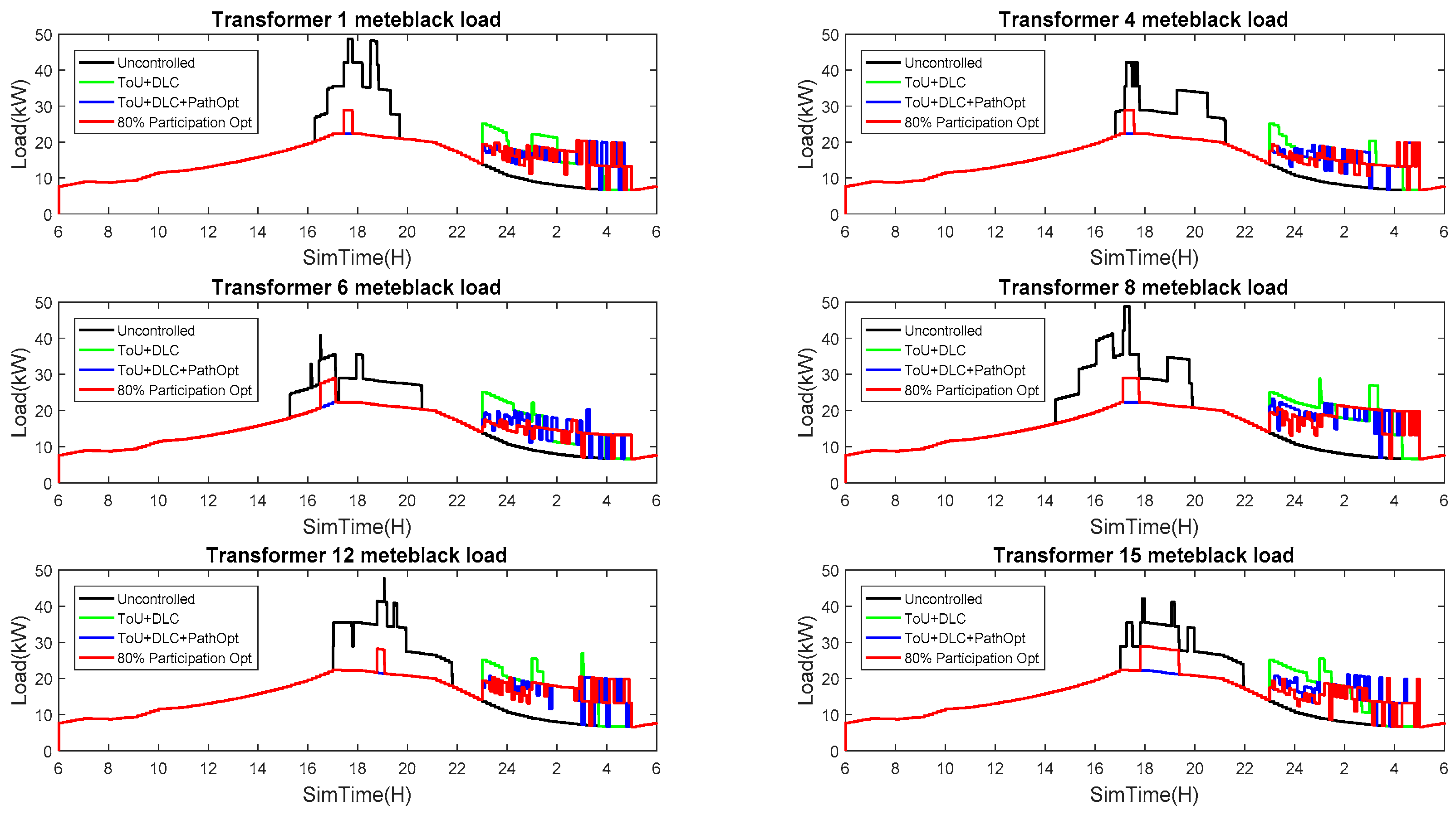
6.2. Load Surge
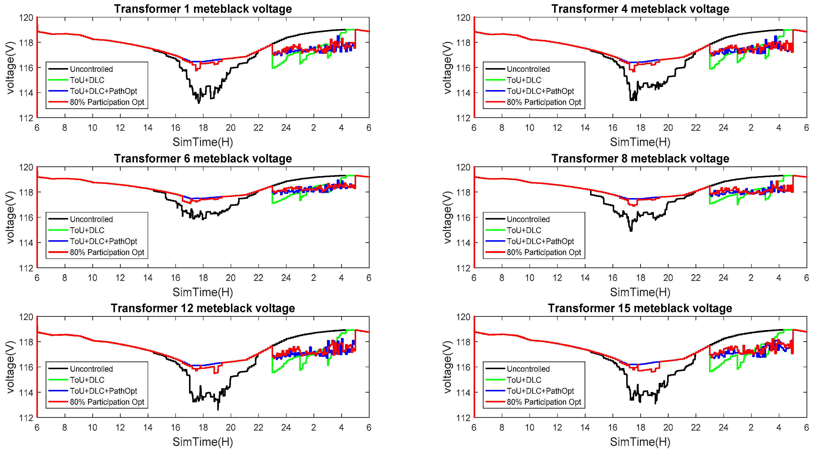
6.3. Voltage Deviation
6.4. Transformer Insulation Aging
6.5. Seasonal Effect
7. Conclusions
Author Contributions
Conflicts of Interest
Appendix A

| Transformer Parameters | Value |
|---|---|
| Winding hottest-spot temperature over top-oil temperature at rated load, | 50 °C |
| Top oil temperature rise over ambient temperature at rated load, | 30 °C |
| Ratio of load loss at rated load to no-load loss, R | 2 |
| Rated load loss | 0.006 (p.u) |
| Weight of the tank | 60 (lb) |
| Weight of core and coil | 50 (lb) |
| Volume of oil | 8.7 (gallon) |
| Winding time constant, | 0.5 (h) |
| exponent, n | 0.8 ONAN |
| exponent, m | 0.8 ONAN |
| Grid Impact | Transformer | January | February | March | April | May | June | July | August | September | October | November | December |
|---|---|---|---|---|---|---|---|---|---|---|---|---|---|
| Load Surge | 1 | 36.5798 | 35.62 | 34.33 | 37.82 | 42.11 | 47.94 | 48.69 | 48.63 | 47.39 | 40.43 | 36.09 | 36.86 |
| 4 | 28.0463 | 27.23 | 26.23 | 31.18 | 35.51 | 41.38 | 42.11 | 42.03 | 40.8 | 33.68 | 27.79 | 28.47 | |
| 6 | 25.6855 | 25.27 | 24.67 | 29.73 | 34.16 | 40.04 | 40.77 | 40.64 | 39.45 | 32.59 | 25.43 | 25.87 | |
| 8 | 33.8089 | 33.12 | 32.27 | 37.62 | 42.1 | 47.98 | 48.71 | 48.62 | 47.4 | 40.28 | 33.58 | 34.18 | |
| 12 | 37.1278 | 36.16 | 34.79 | 37.79 | 41.45 | 47.04 | 47.74 | 47.65 | 46.42 | 40.6 | 36.53 | 37.3 | |
| 15 | 30.5278 | 29.56 | 28.31 | 31.26 | 35.52 | 41.31 | 42.09 | 42.04 | 40.78 | 34 | 29.93 | 30.7 | |
| Minimum line voltage | 1 | 115.6 | 115.8 | 115.2 | 115.8 | 114.4 | 113.3 | 113.2 | 113.2 | 113.4 | 114.7 | 115.7 | 115.6 |
| 4 | 115.9 | 116.1 | 115.4 | 116.1 | 114.6 | 113.5 | 113.4 | 113.4 | 113.6 | 114.9 | 116 | 115.9 | |
| 6 | 117.5 | 117.6 | 117.2 | 117.6 | 116.7 | 115.9 | 115.8 | 115.8 | 116 | 116.9 | 117.5 | 117.4 | |
| 8 | 116.9 | 117 | 116.4 | 117 | 115.8 | 115 | 114.9 | 114.9 | 115.1 | 116 | 116.9 | 116.8 | |
| 12 | 114.7 | 114.9 | 114.6 | 114.9 | 113.9 | 112.7 | 112.6 | 112.6 | 112.9 | 114 | 114.8 | 114.7 | |
| 15 | 115.2 | 115.3 | 115 | 115.3 | 114.3 | 113.2 | 113.1 | 113.1 | 113.4 | 114.5 | 115.3 | 115.1 | |
| Transformer aging—insulation loss of life (%) | 1 | 2.39 × 10⁻⁴ | 1.02 × 10⁻⁴ | 3.95 × 10⁻⁴ | 2.56 × 10⁻³ | 1.48 × 10⁻² | 2.60 × 10⁻¹ | 6.97 × 10⁻¹ | 4.49 × 10⁻¹ | 2.23 × 10⁻¹ | 5.10 × 10⁻³ | 4.54 × 10⁻⁴ | 1.96 × 10⁻⁴ |
| 4 | 2.35 × 10⁻⁵ | 1.09 × 10⁻⁵ | 4.36 × 10⁻⁵ | 2.36 × 10⁻⁴ | 1.10 × 10⁻³ | 2.05 × 10⁻² | 6.56 × 10⁻² | 3.97 × 10⁻² | 1.85 × 10⁻² | 3.79 × 10⁻⁴ | 3.87 × 10⁻⁵ | 1.66 × 10⁻⁵ | |
| 6 | 6.58 × 10⁻⁶ | 2.84 × 10⁻⁶ | 1.76 × 10⁻⁵ | 1.01 × 10⁻⁴ | 5.03 × 10⁻⁴ | 9.87 × 10⁻³ | 3.24 × 10⁻² | 1.90 × 10⁻² | 9.00 × 10⁻³ | 1.62 × 10⁻⁴ | 1.56 × 10⁻⁵ | 4.59 × 10⁻⁶ | |
| 8 | 6.40 × 10⁻⁵ | 2.97 × 10⁻⁵ | 1.69 × 10⁻⁴ | 1.34 × 10⁻³ | 7.70 × 10⁻³ | 1.34 × 10⁻¹ | 3.77 × 10⁻¹ | 2.40 × 10⁻¹ | 1.22 × 10⁻¹ | 2.50 × 10⁻³ | 1.66 × 10⁻⁴ | 4.37 × 10⁻⁵ | |
| 12 | 9.53 × 10⁻⁵ | 3.97 × 10⁻⁵ | 1.37 × 10⁻⁴ | 7.21 × 10⁻⁴ | 3.90 × 10⁻³ | 6.93 × 10⁻² | 2.07 × 10⁻¹ | 1.31 × 10⁻¹ | 6.24 × 10⁻² | 1.40 × 10⁻³ | 4.69 × 10⁻⁵ | 7.43 × 10⁻⁵ | |
| 15 | 3.22 × 10⁻⁵ | 1.33 × 10⁻⁵ | 5.43 × 10⁻⁵ | 2.86 × 10⁻⁴ | 1.50 × 10⁻³ | 2.84 × 10⁻² | 8.87 × 10⁻² | 5.42 × 10⁻² | 2.53 × 10⁻² | 5.10 × 10⁻⁴ | 5.45 × 10⁻⁵ | 2.47 × 10⁻⁵ |
| Grid Impact | Transformer | January | February | March | April | May | June | July | August | September | October | November | December |
|---|---|---|---|---|---|---|---|---|---|---|---|---|---|
| Load Surge | 1 | 18.67 | 18.71 | 18.39 | 17.81 | 19.99 | 23.31 | 25.14 | 24.34 | 22.29 | 18.94 | 18.16 | 18.52 |
| 4 | 18.67 | 18.71 | 18.39 | 17.81 | 19.99 | 23.31 | 25.14 | 23.34 | 22.29 | 18.94 | 18.16 | 18.52 | |
| 6 | 18.67 | 18.71 | 18.39 | 17.81 | 19.99 | 23.31 | 25.14 | 23.34 | 22.29 | 18.94 | 18.16 | 18.52 | |
| 8 | 23.68 | 23.74 | 23.35 | 23.05 | 24.3 | 26.62 | 28.79 | 28.07 | 27.09 | 23.99 | 23.3 | 23.62 | |
| 12 | 22.84 | 22.91 | 22.75 | 22.5 | 22.98 | 24.85 | 26.95 | 26.45 | 25.58 | 23.04 | 22.41 | 22.79 | |
| 15 | 20.28 | 20.44 | 20.25 | 19.75 | 21 | 23.31 | 25.49 | 24.77 | 23.79 | 20.69 | 20 | 20.32 | |
| Minimum line voltage | 1 | 117.1 | 117 | 117.1 | 117.2 | 116.8 | 116.3 | 116 | 116.1 | 116.3 | 117 | 117.1 | 117.1 |
| 4 | 117 | 117 | 117 | 117.1 | 116.8 | 116.2 | 115.9 | 116 | 116.3 | 117 | 117.1 | 117 | |
| 6 | 117.9 | 117.9 | 117.9 | 118 | 117.7 | 117.3 | 117.1 | 117.2 | 117.4 | 117.9 | 118 | 117.9 | |
| 8 | 117.6 | 117.6 | 117.7 | 117.7 | 117.6 | 117.3 | 117 | 117.1 | 117.2 | 117.6 | 117.7 | 117.6 | |
| 12 | 116.7 | 116.7 | 116.7 | 116.8 | 116.5 | 115.9 | 115.6 | 115.7 | 116.1 | 116.7 | 116.8 | 116.7 | |
| 15 | 116.9 | 116.7 | 116.8 | 116.9 | 116.6 | 116 | 115.7 | 115.8 | 116.1 | 116.6 | 116.8 | 116.8 | |
| Transformer Aging—insulation loss of life (%) | 1 | 2.51 × 10⁻⁶ | 1.06 × 10⁻⁶ | 3.81 × 10⁻⁶ | 1.25 × 10⁻⁵ | 2.66 × 10⁻⁵ | 4.08 × 10⁻⁴ | 1.80 × 10⁻³ | 9.30 × 10⁻⁴ | 4.28 × 10⁻⁴ | 1.33 × 10⁻⁵ | 3.45 × 10⁻⁶ | 2.07 × 10⁻⁶ |
| 4 | 1.54 × 10⁻⁶ | 6.40 × 10⁻⁷ | 3.81 × 10⁻⁶ | 1.02 × 10⁻⁵ | 2.44 × 10⁻⁵ | 3.88 × 10⁻⁴ | 1.70 × 10⁻³ | 8.55 × 10⁻⁴ | 3.94 × 10⁻⁴ | 1.08 × 10⁻⁵ | 3.45 × 10⁻⁶ | 1.22 × 10⁻⁶ | |
| 6 | 2.18 × 10⁻⁶ | 9.22 × 10⁻⁷ | 4.70 × 10⁻⁶ | 1.17 × 10⁻⁵ | 2.62 × 10⁻⁵ | 4.07 × 10⁻⁴ | 1.80 × 10⁻³ | 9.20 × 10⁻⁴ | 4.23 × 10⁻⁴ | 1.25 × 10⁻⁵ | 3.20 × 10⁻⁶ | 1.74 × 10⁻⁶ | |
| 8 | 4.63 × 10⁻⁶ | 1.98 × 10⁻⁶ | 8.33 × 10⁻⁶ | 1.72 × 10⁻⁵ | 3.04 × 10⁻⁵ | 4.33 × 10⁻⁴ | 2.10 × 10⁻³ | 1.00 × 10⁻³ | 4.79 × 10⁻⁴ | 1.80 × 10⁻⁵ | 3.85 × 10⁻⁶ | 4.15 × 10⁻⁶ | |
| 12 | 2.98 × 10⁻⁶ | 1.26 × 10⁻⁶ | 5.97 × 10⁻⁶ | 1.35 × 10⁻⁵ | 2.74 × 10⁻⁵ | 4.13 × 10⁻⁴ | 1.90 × 10⁻³ | 9.56 × 10⁻⁴ | 4.40 × 10⁻⁴ | 1.44 × 10⁻⁵ | 3.85 × 10⁻⁶ | 2.53 × 10⁻⁶ | |
| 15 | 2.93 × 10⁻⁶ | 1.24 × 10⁻⁶ | 5.86 × 10⁻⁶ | 1.33 × 10⁻⁵ | 2.76 × 10⁻⁵ | 4.18 × 10⁻⁴ | 1.90 × 10⁻³ | 9.68 × 10⁻⁴ | 4.45 × 10⁻⁴ | 1.44 × 10⁻⁵ | 3.82 × 10⁻⁶ | 2.42E-06 |
| Grid Impact | Transformer | January | February | March | April | May | June | July | August | September | October | November | December |
|---|---|---|---|---|---|---|---|---|---|---|---|---|---|
| Load Surge | 1 | 16.77 | 16.64 | 16.13 | 16.13 | 17.01 | 21.59 | 22.32 | 22.24 | 21 | 16.42 | 15.74 | 16.19 |
| 4 | 16.22 | 16.29 | 16.13 | 15.9 | 16.29 | 21.59 | 22.32 | 22.24 | 21 | 16.42 | 15.78 | 16.18 | |
| 6 | 16.21 | 16.3 | 16.12 | 15.89 | 16.12 | 21.59 | 22.32 | 22.24 | 21 | 16.42 | 15.74 | 16.18 | |
| 8 | 16.46 | 19.68 | 16.12 | 16.13 | 22.57 | 24.42 | 22.32 | 22.24 | 21 | 19.96 | 19.25 | 20.32 | |
| 12 | 16.27 | 16.3 | 16.12 | 16.03 | 16.2 | 21.59 | 22.32 | 22.24 | 21 | 16.5 | 16.4 | 16.27 | |
| 15 | 16.23 | 16.29 | 16.26 | 16.13 | 16.3 | 21.59 | 22.32 | 22.24 | 21 | 16.5 | 15.74 | 16.27 | |
| Minimum line voltage | 1 | 117.5 | 117.6 | 117.5 | 117.7 | 117.5 | 116.6 | 116.5 | 116.5 | 116.7 | 117.7 | 117.8 | 117.7 |
| 4 | 117.5 | 117.6 | 117.5 | 117.7 | 117.5 | 116.5 | 116.4 | 116.4 | 116.6 | 117.7 | 117.9 | 117.7 | |
| 6 | 118.3 | 118.3 | 118.4 | 118.3 | 118.3 | 117.6 | 117.5 | 117.5 | 117.6 | 118.3 | 118.5 | 118.4 | |
| 8 | 118.2 | 118.2 | 118.3 | 118 | 118 | 117.6 | 117.5 | 117.5 | 117.6 | 118 | 118.4 | 118.2 | |
| 12 | 117.2 | 117.3 | 117.3 | 117.5 | 117.3 | 116.3 | 116.1 | 116.1 | 116.4 | 117.4 | 117.6 | 117.5 | |
| 15 | 117.3 | 117.4 | 117.4 | 117.6 | 117.3 | 116.3 | 116.2 | 116.2 | 116.4 | 117.5 | 117.7 | 117.6 | |
| Transformer Aging—insulation loss of life (%) | 1 | 1.42 × 10⁻⁶ | 5.93 × 10⁻⁷ | 3.81 × 10⁻⁶ | 9.78 × 10⁻⁶ | 2.37 × 10⁻⁵ | 3.76 × 10⁻⁴ | 1.60 × 10⁻³ | 8.26 × 10⁻⁴ | 3.81 × 10⁻⁴ | 1.04 × 10⁻⁵ | 2.51 × 10⁻⁶ | 1.25 × 10⁻⁶ |
| 4 | 1.21 × 10⁻⁶ | 4.93 × 10⁻⁷ | 3.81 × 10⁻⁶ | 9.36 × 10⁻⁶ | 2.32 × 10⁻⁵ | 3.73 × 10⁻⁴ | 1.60 × 10⁻³ | 8.08 × 10⁻⁴ | 3.73 × 10⁻⁴ | 9.78 × 10⁻⁶ | 2.31 × 10⁻⁶ | 9.90 × 10⁻⁷ | |
| 6 | 1.15 × 10⁻⁶ | 4.90 × 10⁻⁷ | 4.70 × 10⁻⁶ | 9.14 × 10⁻⁶ | 2.32 × 10⁻⁵ | 3.73 × 10⁻⁴ | 1.60 × 10⁻³ | 8.06 × 10⁻⁴ | 3.75 × 10⁻⁴ | 9.91 × 10⁻⁶ | 2.31 × 10⁻⁶ | 9.26 × 10⁻⁷ | |
| 8 | 2.72 × 10⁻⁶ | 1.14 × 10⁻⁶ | 8.33 × 10⁻⁶ | 1.37 × 10⁻⁵ | 2.59 × 10⁻⁵ | 3.91 × 10⁻⁴ | 1.80 × 10⁻³ | 8.91 × 10⁻⁴ | 4.05 × 10⁻⁴ | 1.33 × 10⁻⁵ | 3.59 × 10⁻⁶ | 2.65 × 10⁻⁶ | |
| 12 | 1.65 × 10⁻⁶ | 6.61 × 10⁻⁷ | 5.97 × 10⁻⁶ | 1.04 × 10⁻⁵ | 2.41 × 10⁻⁵ | 3.78 × 10⁻⁴ | 1.60 × 10⁻³ | 8.38 × 10⁻⁴ | 3.92 × 10⁻⁴ | 1.09 × 10⁻⁵ | 2.72 × 10⁻⁶ | 1.43 × 10⁻⁶ | |
| 15 | 1.35 × 10⁻⁶ | 5.51 × 10⁻⁷ | 5.86 × 10⁻⁶ | 9.68 × 10⁻⁶ | 2.37 × 10⁻⁵ | 3.75 × 10⁻⁴ | 1.60 × 10⁻³ | 8.27 × 10⁻⁴ | 3.84 × 10⁻⁴ | 1.03 × 10⁻⁵ | 2.48 × 10⁻⁶ | 1.21 × 10⁻⁶ |
| Grid Impact | Transformer | January | February | March | April | May | June | July | August | September | October | November | December |
|---|---|---|---|---|---|---|---|---|---|---|---|---|---|
| Load Surge | 1 | 16.24 | 16.31 | 16.14 | 17.98 | 22.31 | 28.13 | 28.91 | 28.83 | 27.6 | 20.71 | 15.74 | 16.44 |
| 4 | 16.22 | 16.29 | 16.13 | 17.9 | 22.31 | 28.16 | 28.91 | 28.83 | 27.6 | 20.56 | 15.78 | 16.18 | |
| 6 | 16.22 | 16.3 | 12.96 | 17.65 | 22.3 | 28.19 | 28.92 | 28.82 | 27.61 | 20.41 | 15.74 | 13.49 | |
| 8 | 16.77 | 17.04 | 16.34 | 17.65 | 22.31 | 28.19 | 28.92 | 28.83 | 27.61 | 20.71 | 22.34 | 22.78 | |
| 12 | 16.38 | 16.42 | 16.19 | 17.96 | 21.88 | 27.52 | 28.26 | 28.18 | 26.94 | 20.81 | 16.73 | 17.5 | |
| 15 | 17.23 | 16.51 | 14.55 | 18.15 | 22.31 | 28.13 | 28.89 | 28.83 | 27.59 | 20.82 | 16.64 | 17.5 | |
| Minimum line voltage | 1 | 117.5 | 117.8 | 117.5 | 117.6 | 116.9 | 115.9 | 115.7 | 115.8 | 116 | 117.1 | 117.8 | 117.7 |
| 4 | 117.5 | 117.6 | 117.5 | 117.5 | 116.8 | 115.8 | 115.7 | 115.7 | 115.9 | 117.1 | 117.7 | 117.7 | |
| 6 | 118.3 | 118.3 | 118.4 | 118.5 | 117.9 | 117.2 | 117.1 | 117.1 | 117.3 | 118.1 | 118.5 | 118.6 | |
| 8 | 118.3 | 118.3 | 118.3 | 118.2 | 117.7 | 117 | 116.9 | 116.9 | 117.1 | 117.9 | 118.1 | 118 | |
| 12 | 117.3 | 117.4 | 117.3 | 117.4 | 116.7 | 115.6 | 115.5 | 115.5 | 115.8 | 116.9 | 117.6 | 117.5 | |
| 15 | 117.3 | 117.5 | 117.4 | 117.4 | 116.8 | 115.7 | 115.6 | 115.6 | 115.9 | 117 | 117.7 | 117.5 | |
| Transformer Aging—insulation loss of life (%) | 1 | 1.49 × 10⁻⁶ | 5.88 × 10⁻⁷ | 3.81 × 10⁻⁶ | 1.11 × 10⁻⁵ | 3.03 × 10⁻⁵ | 5.09 × 10⁻⁴ | 2.10 × 10⁻³ | 1.10 × 10⁻³ | 4.99 × 10⁻⁴ | 1.21 × 10⁻⁵ | 2.66 × 10⁻⁶ | 1.23 × 10⁻⁶ |
| 4 | 1.27 × 10⁻⁶ | 4.93 × 10⁻⁷ | 3.81 × 10⁻⁶ | 1.06 × 10⁻⁵ | 3.01 × 10⁻⁵ | 5.08 × 10⁻⁴ | 2.00 × 10⁻³ | 1.10 × 10⁻³ | 4.94 × 10⁻⁴ | 1.17 × 10⁻⁵ | 2.49 × 10⁻⁶ | 1.00 × 10⁻⁶ | |
| 6 | 1.13 × 10⁻⁶ | 4.84 × 10⁻⁷ | 4.70 × 10⁻⁶ | 1.14 × 10⁻⁵ | 3.45 × 10⁻⁵ | 5.85 × 10⁻⁴ | 2.30 × 10⁻³ | 1.20 × 10⁻³ | 5.70 × 10⁻⁴ | 1.29 × 10⁻⁵ | 2.56 × 10⁻⁶ | 8.62 × 10⁻⁷ | |
| 8 | 2.43 × 10⁻⁶ | 9.97 × 10⁻⁷ | 8.33 × 10⁻⁶ | 1.52 × 10⁻⁵ | 4.05 × 10⁻⁵ | 4.05 × 10⁻⁵ | 2.80 × 10⁻³ | 1.50 × 10⁻³ | 6.74 × 10⁻⁴ | 1.67 × 10⁻⁵ | 3.81 × 10⁻⁶ | 2.31 × 10⁻⁶ | |
| 12 | 1.80 × 10⁻⁶ | 6.71 × 10⁻⁷ | 5.97 × 10⁻⁶ | 1.12 × 10⁻⁵ | 2.82 × 10⁻⁵ | 6.93 × 10⁻⁴ | 1.90 × 10⁻³ | 1.00 × 10⁻³ | 4.61 × 10⁻⁴ | 1.20 × 10⁻⁵ | 2.88 × 10⁻⁶ | 1.49 × 10⁻⁶ | |
| 15 | 2.00 × 10⁻⁶ | 8.17 × 10⁻⁷ | 5.86 × 10⁻⁶ | 1.87 × 10⁻⁵ | 7.17 × 10⁻⁵ | 1.37 × 10⁻³ | 5.00 × 10⁻³ | 2.80 × 10⁻³ | 1.30 × 10⁻³ | 2.51 × 10⁻⁵ | 4.06 × 10⁻⁶ | 1.56 × 10⁻⁶ |
References
- United States Environmental Protection Agency (EPA), National Highway Traffic Safety Administration (NHTSA). 2017 and Later Model Year Light-Duty Vehicle Greenhouse Gas Emissions and Corporate Average Fuel Economy Standards. 2011. Available online: https://www.gpo.gov/fdsys/search/pagedetails.action?collectionCode=FR&browsePath=2011%2F12%2F12-01%5C%2F5%2FEnvironmental+Protection+Agency&granuleId=2011-30358&packageId=FR-2011-12-01&fromBrowse=true (accessed on 30 November 2016). [Google Scholar]
- U.S. Department of State. United States Climate Action Report (2014 CAR). Available online: http://www.state.gov/e/oes/rls/rpts/car6/index.htm (accessed on 30 November 2016).
- U.S. Environmental Protection Agency. Inventory of U.S. Greenhouse Gas Emissions and Sinks. 2015. Available online: http://www.epa.gov/climatechange/emissions/usinventoryreport.html (accessed on 30 November 2016). [Google Scholar]
- Liu, R.; Dow, L.; Liu, E. A survey of PEV impacts on electric utilities. In Proceedings of the 2011 IEEE PES Innovative Smart Grid Technologies (ISGT), Anaheim, CA, USA, 17–19 January 2011; pp. 1–8.
- Bosovic, A.; Music, M.; Sadovic, S. Analysis of the impacts of plug-in electric vehicle charging on the part of a real medium voltage distribution network. In Proceedings of the 2014 IEEE PES Innovative Smart Grid Technologies Conference Europe (ISGT-Europe), Istanbul, Turkey, 12–15 October 2014; pp. 1–7.
- Calderaro, V.; Galdi, V.; Graber, G.; Massa, G.; Piccolo, A. Plug-in EV charging impact on grid based on vehicles usage data. In Proceedings of the 2014 IEEE International Electric Vehicle Conference (IEVC), Florence, Italy, 17–19 December 2014; pp. 1–7.
- Qian, K.; Zhou, C.; Allan, M.; Yuan, Y. Modeling of Load Demand Due to EV Battery Charging in Distribution Systems. IEEE Trans. Power Syst. 2011, 26, 802–810. [Google Scholar] [CrossRef]
- Rautiainen, A.; Repo, S.; Järventausta, P.; Mutanen, A.; Vuorilehto, K.; Jalkanen, K. Statistical Charging Load Modeling of PHEVs in Electricity Distribution Networks Using National Travel Survey Data. IEEE Trans. Smart Grid 2012, 3, 1650–1659. [Google Scholar] [CrossRef]
- Argade, S.; Aravinthan, V.; Jewell, W. Probabilistic modeling of EV charging and its impact on distribution transformer loss of life. In Proceedings of the 2012 IEEE International Electric Vehicle Conference (IEVC), Greenville, SC, USA, 4–8 March 2012; pp. 1–8.
- Hilshey, A.D.; Rezaei, P.; Hines, P.D.H.; Frolik, J. Electric vehicle charging: Transformer impacts and smart, decentralized solutions. In Proceedings of the 2012 IEEE Power and Energy Society General Meeting, San Diego, CA, USA, 22–26 July 2012; pp. 1–8.
- Meyer, D.; Choi, J.; Wang, J. Increasing EV public charging with distributed generation in the electric grid. In Proceedings of the 2015 IEEE Transportation Electrification Conference and Expo (ITEC), Dearborn, MI, USA, 14–17 June 2015; pp. 1–6.
- Vehicle-Grid Integration: A Vision for Zero-Emission Transportation Interconnected throughout California’s Electricity System. 2013. Available online: http://docs.cpuc.ca.gov/PublishedDocs/Published/G000/M080/K775/80775679.pdf (accessed on 30 November 2016).
- Scholer, R.A.; McGlynn, H. Smart Charging Standards for Plug-In Electric Vehicles. In Proceedings of the SAE 2014 World Congress & Exhibition, Detroit, MI, USA, 8–10 April 2014.
- Kersting, W.H. Distribution System Modeling and Analysis, 2nd ed.; CRC Press: Boca Raton, FL, USA, 2002. [Google Scholar]
- American National Standards Institute (ANSI). American National Standard For Electric Power Systems and Equipment—Voltage Ratings (60 Hertz); ANSI C84.1-2011; National Electrical Manufacturers Association: Rosslyn, VA, USA, 2011. [Google Scholar]
- GridLAB-D. Available online: http://www.gridlabd.org/ (accessed on 30 November 2016).
- Florida Public Service Commission. Report on Electric Vehicle Charging. Tallahassee, FL, USA. 2012. Available online: http://www.freshfromflorida.com/content/download/11426/144852/Electric_Vehicle_Charging_Report.pdf (accessed on 30 November 2016).
- National Highway Traffic Safety Administration (NHTSA). National Household Travel Survey. Available online: http://nhts.ornl.gov/index.shtml (accessed on 30 November 2016).
- CEl-Bayeh, L.Z.; Mougharbel, I.; Saad, M.; Chandra, A.; Lefebvre, S.; Asber, D. A detailed review on the parameters to be considered for an accurate estimation on the Plug-in Electric Vehicle’s final State of Charge. In Proceedings of the 2016 3rd International Conference on Renewable Energies for Developing Countries (REDEC), Beirut, Lebanon, 13–15 July 2016; pp. 1–6.
- SAE World Congress. J1772-SAE Electric Vehicle and Plug in Hybrid Electric Vehicle Conductive Charge Coupler. 2010. Available online: http://standards.sae.org/wip/j1772/ (accessed on 30 November 2016).
- IEEE Power & Energy Socierty (PES). IEEE 13 Node Test Feeder. Available online: http://ewh.ieee.org/soc/pes/dsacom/testfeeders/index.html (accessed on 30 November 2016).
- Kersting, W.H. Radial distribution test feeders. In Proceedings of the IEEE Power Engineering Society Winter Meeting, Columbus, OH, USA, 28 January–1 February 2001.
- Office of Energy Efficiency & Renewable Energy (EERE). Commercial and Residential Hourly Load Profiles for all TMY3 Locations in the United States. Available online: http://en.openei.org/doe-opendata/dataset/commercial-and-residential-hourly-load-profiles-for-all-tmy3-locations-in-the-united-states (accessed on 30 November 2016).
- C57.91-2011—IEEE Guide for Loading Mineral-Oil-Immersed Transformers and Step-Voltage Regulators. 2012. Available online: http://ieeexplore.ieee.org/servlet/opac?punumber=6166925 (accessed on 30 November 2016).
- Gönen, T. Electric Power Distribution System Engineering, 3rd ed.; CRC Press: Boca Raton, FL, USA, 2008. [Google Scholar]
- GridLAB-D: Power Flow User Guide. Available online: http://gridlabd.me.uvic.ca/wiki/index.php/Power_Flow_User_Guide (accessed on 30 November 2016).


| Month | Average Load (kW) | Temperature High (F) | Temperature Low (F) |
|---|---|---|---|
| January | 0.97 | 67 | 46 |
| February | 0.95 | 71 | 49 |
| March | 0.86 | 77 | 53 |
| April | 1.05 | 85 | 60 |
| May | 1.39 | 95 | 69 |
| June | 1.99 | 104 | 78 |
| July | 2.25 | 106 | 83 |
| August | 2.17 | 104 | 83 |
| September | 2.01 | 100 | 77 |
| October | 1.33 | 89 | 65 |
| November | 0.88 | 76 | 53 |
| December | 0.96 | 65 | 45 |
| Loss of Life in One Day | T1 1 (10−3) | T4 (10−3) | T6 (10−3) | T8 (10−3) | T12 (10−3) | T15 (10−3) |
|---|---|---|---|---|---|---|
| Uncontrolled charging | 700 | 66 | 32 | 377 | 207 | 89 |
| ToU + DLC charging | 1.80 | 1.70 | 1.80 | 2.10 | 1.90 | 1.90 |
| ToU + DLC + optimal control charging | 1.60 | 1.60 | 1.60 | 1.80 | 1.60 | 1.60 |
| 80% participation rate of optimal control charging (20% uncontrolled charging) | 2.10 | 2.00 | 2.30 | 2.80 | 1.90 | 5.00 |
© 2016 by the authors; licensee MDPI, Basel, Switzerland. This article is an open access article distributed under the terms and conditions of the Creative Commons Attribution (CC-BY) license (http://creativecommons.org/licenses/by/4.0/).
Share and Cite
Cao, C.; Wang, L.; Chen, B. Mitigation of the Impact of High Plug-in Electric Vehicle Penetration on Residential Distribution Grid Using Smart Charging Strategies. Energies 2016, 9, 1024. https://doi.org/10.3390/en9121024
Cao C, Wang L, Chen B. Mitigation of the Impact of High Plug-in Electric Vehicle Penetration on Residential Distribution Grid Using Smart Charging Strategies. Energies. 2016; 9(12):1024. https://doi.org/10.3390/en9121024
Chicago/Turabian StyleCao, Chong, Luting Wang, and Bo Chen. 2016. "Mitigation of the Impact of High Plug-in Electric Vehicle Penetration on Residential Distribution Grid Using Smart Charging Strategies" Energies 9, no. 12: 1024. https://doi.org/10.3390/en9121024
APA StyleCao, C., Wang, L., & Chen, B. (2016). Mitigation of the Impact of High Plug-in Electric Vehicle Penetration on Residential Distribution Grid Using Smart Charging Strategies. Energies, 9(12), 1024. https://doi.org/10.3390/en9121024