Article

Analytical Modeling of Static Eccentricities in Axial Flux Permanent-Magnet Machines with Concentrated Windings

1
Engineering Research Center for Motion Control of Ministry of Education, Southeast University, Nanjing 210096, China
2
Department of Electrical Energy, Systems and Automation, Ghent University, Ghent B-9000, Belgium
*
Author to whom correspondence should be addressed.
Energies 2016, 9(11), 892; https://doi.org/10.3390/en9110892
Submission received: 7 July 2016 / Revised: 23 October 2016 / Accepted: 24 October 2016 / Published: 29 October 2016
(This article belongs to the Collection Electric and Hybrid Vehicles Collection)

Abstract

:
The aim of this paper is to calculate the static eccentricity (SE) of a double rotor axial flux permanent magnet (AFPM) machine by using a general analytical model. The flux density in the air gap under healthy conditions is calculated firstly, where the axial and circumferential magnetic flux densities are obtained using a coupled solution of Maxwell’s equations and Schwarz-Christoffel (SC) mapping. The magnetic flux densities under SE conditions are calculated afterwards using a novel bilinear mapping. Some important electromagnetic parameters, e.g., back electromotive force (EMF), cogging torque and electromagnetic (EM) torque, are calculated for both SE and healthy conditions, and compared with the finite element (FE) model. As for the double rotor AFPM, SE does not contribute much effect on the back EMF and EM torque, while the cogging torque is increased. At each calculated section, FE models were built to validate the analytical model. The results show that the analytical predictions agree well with the FE results. Finally, the results of analytical model are verified via experimental results.

1. Introduction

Axial flux permanent magnet machines (AFPMMs) have a number of distinct advantages over radial flux permanent magnet machines (RFPMMs). Axial flux permanent magnet (AFPM) can be designed to have a higher power-to-weight ratio, resulting in a need for less core material and reduced complexity to adjust the air gap [1]. Moreover, because of the disc shaped rotor and stator structure, an AFPM is smaller in size than its RFPMMs counterparts. This particular structural characteristic makes it easy to address the space limitation in some applications such as electric vehicles (EV) [2], hybrid electric vehicles (HEV) [3], wind turbos [4] and flywheel storage systems [5], etc.
However, due to the smaller contact surface between the rotor and the shaft, it is more difficult to design a rotor-shaft mechanical joint with a high mechanical integrity [6], which makes AFPMMs more susceptible to imperfect assembly issues such as static eccentricities (SEs), dynamic angular misalignment [7] and static/dynamic eccentricity misalignment [8]. Under angular eccentric conditions, the rotor is inclined and the air gap is asymmetric. If the rotor shaft assembly is sufficiently rigid, which means that the level of static eccentricity (SE) does not change during periodic operation, the axial force becomes unbalanced causing vibrations and unbalanced magnetic forces (UMFs). This leads to deterioration of both the machine’s performance and lifetime. The UMFs can also act on the stator core, exposing the stator windings to unnecessary and potentially harmful vibrations and in the most extreme case, causing the stator and the rotor to scrape [9]. It is therefore important to estimate SE by measuring some suitable machine quantities.
Various techniques could be used for modeling AFPMMs under SE conditions, e.g., an analytical model [10], finite element (FE) model [11], magnetic equivalent circuit (MEC) [12] or a combination of these methods. The 3D-FE model can precisely model the influence of eccentricity owing to the accurate computation of air gap region, but it is time consuming, thus, some references have proposed alternative methods to reduce the computation time. The quasi-3D method, which is widely adopted by AFPM designers, still takes a large amount of computation time for SEs [13]. Another alternative approach is the field reconstruction (FR) method [14,15]. The FR method is a mixed analytical-FE method and partly depends on the FE model. Although, it is much faster than the 3D-FE model, it still takes a lot of time for modeling the different SE geometries. The analytical approach, due to its fast and acceptable results, is regarded as an efficient and favorable method compared to the other methods mentioned above.
Analytical solutions are categorized in different groups. One group is based on the MEC [12]. The MEC is not accurate enough for some qualities like cogging torque and forces because of the nodes limit. In addition, the model needs to be rearranged at each simulation step due to the requirement of alignment between stator and rotor reluctances. Moreover, it is more complex when dealing with the non-uniform air gap. Other possible analytical solutions are appearing in the literature [16], but the methods used in both papers ignored the circumferential flux density when modeling SE conditions. The Conformal Mapping (CM) method has so far not been used for accurate magnetic field analysis for AFPMSMs. In [17], Zarko used this method to calculate the relative permeability of the air gap considering the slotting effect, but one of the main assumptions is that the motors have an infinite slot opening which implies the shape of slot is ignored. Following this paper, Zarko improved this method in [18] to handle this problem, but the computational complexity increases as well.
To overcome the aforementioned problems, this paper adopts an accurate and improved CM method combined with the Schwarz-Christoffel (SC) method for the no-load and on-load conditions under SEs. This method depends on the Matlab SC Toolbox instead of the FE model [19].
This paper is organized as follows: in Section 2, a description of double rotor prototype AFPM with concentrated coil is provided. Section 3 introduces the electromagnetic calculations and SC transformation used in this paper. SE and its effects on magnetic field are also described in this section. Afterward, the models of both the healthy condition and the static eccentric magnetic distribution are introduced in Section 4. In Section 5, the simulation results, e.g., the back electromotive force (EMF), cogging torque and EM torque, are compared and validated through the simulations done by the FE model developed by the commercial software JMAG (https://www.jmag-international.com/). In Section 6, the experimental results verify the accuracy of this method, which is followed by a brief summary and conclusion of the current study.

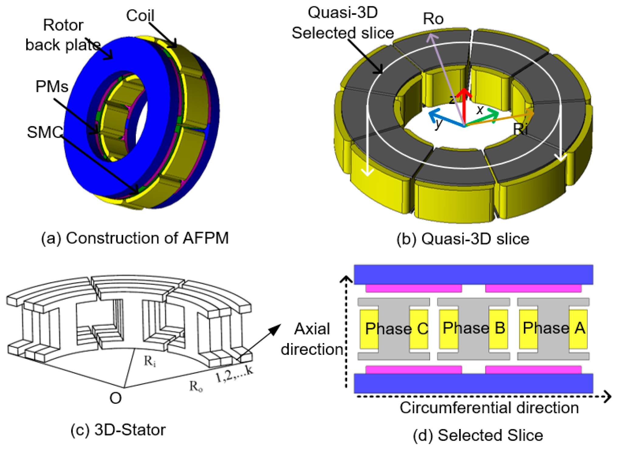
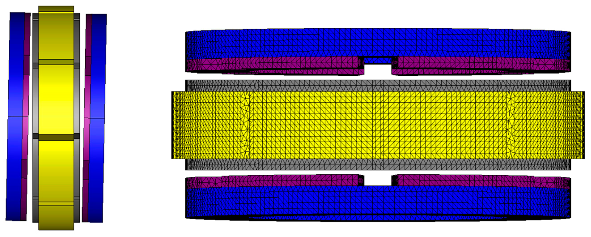
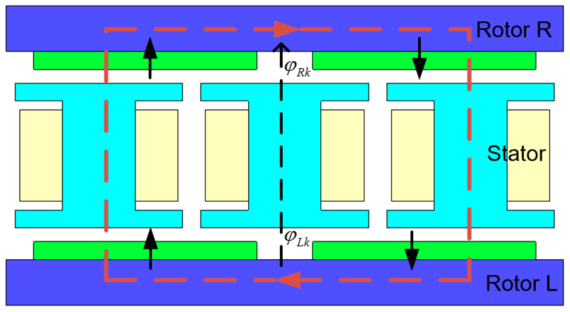
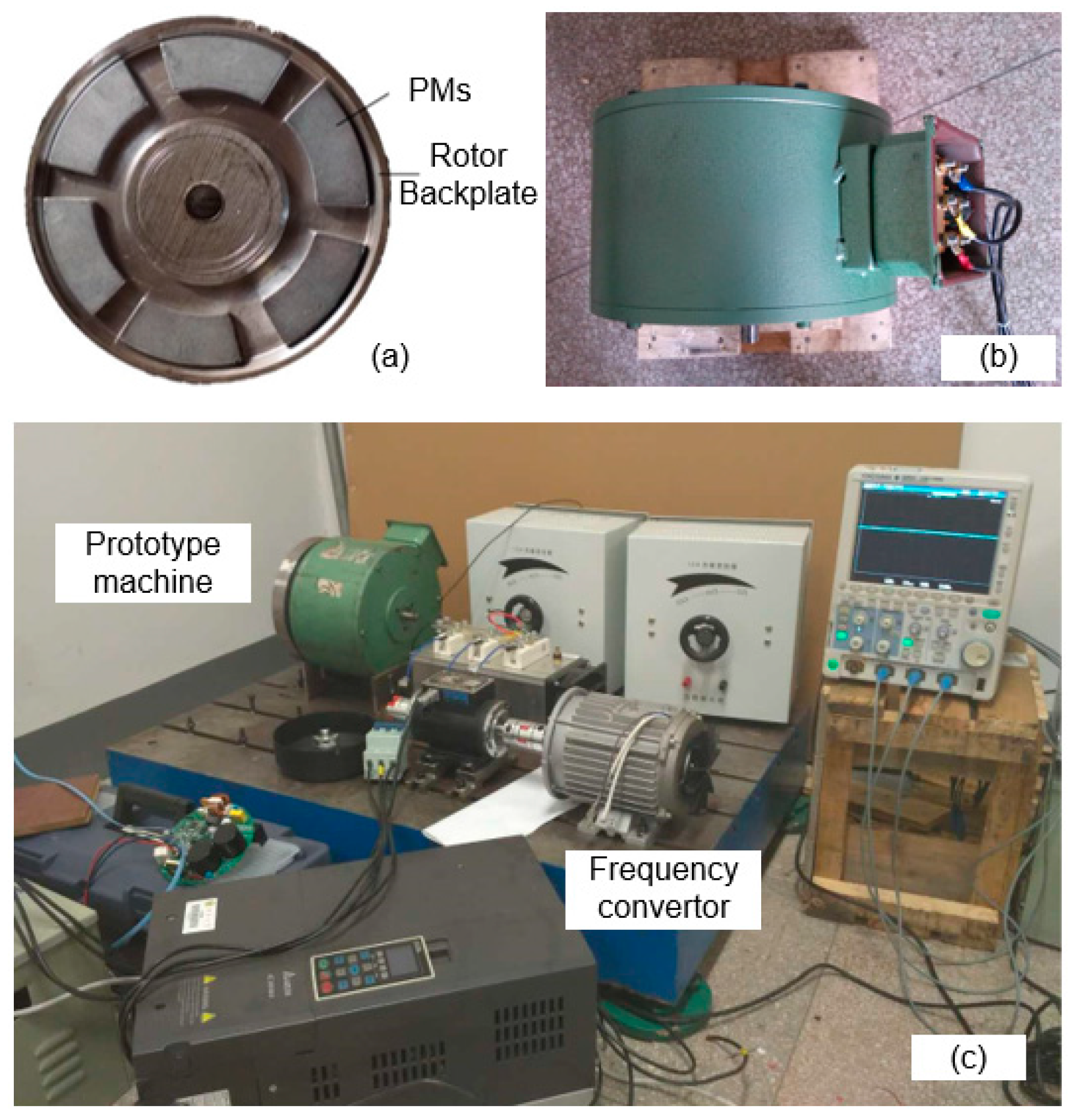
2. Description of the Prototype Axial Flux Permanent Magnet Machine

Figure 1a shows the construction of the test machine used in this paper. The AFPM machine consists of two rotors and one segmented stator. Soft magnetic composite (SMC) is used for the stator core and axially magnetized NdFeB permanent magnets (PMs) are mounted on the surface of each rotor, which is made of #45 steel, the SMC modules are fastened by resin and holders. Three phase concentrated windings are distributed on each stator segment to avoid overlapping. This machine topology benefits from advantages including short end windings with high winding fill factor, small stator iron loss under high-speed operation and a convenient manufacturing and assembly process, plus reduced stator weight due to the absence of the stator yoke. The dimensions and specifications of the investigated machine are shown in Table 1.

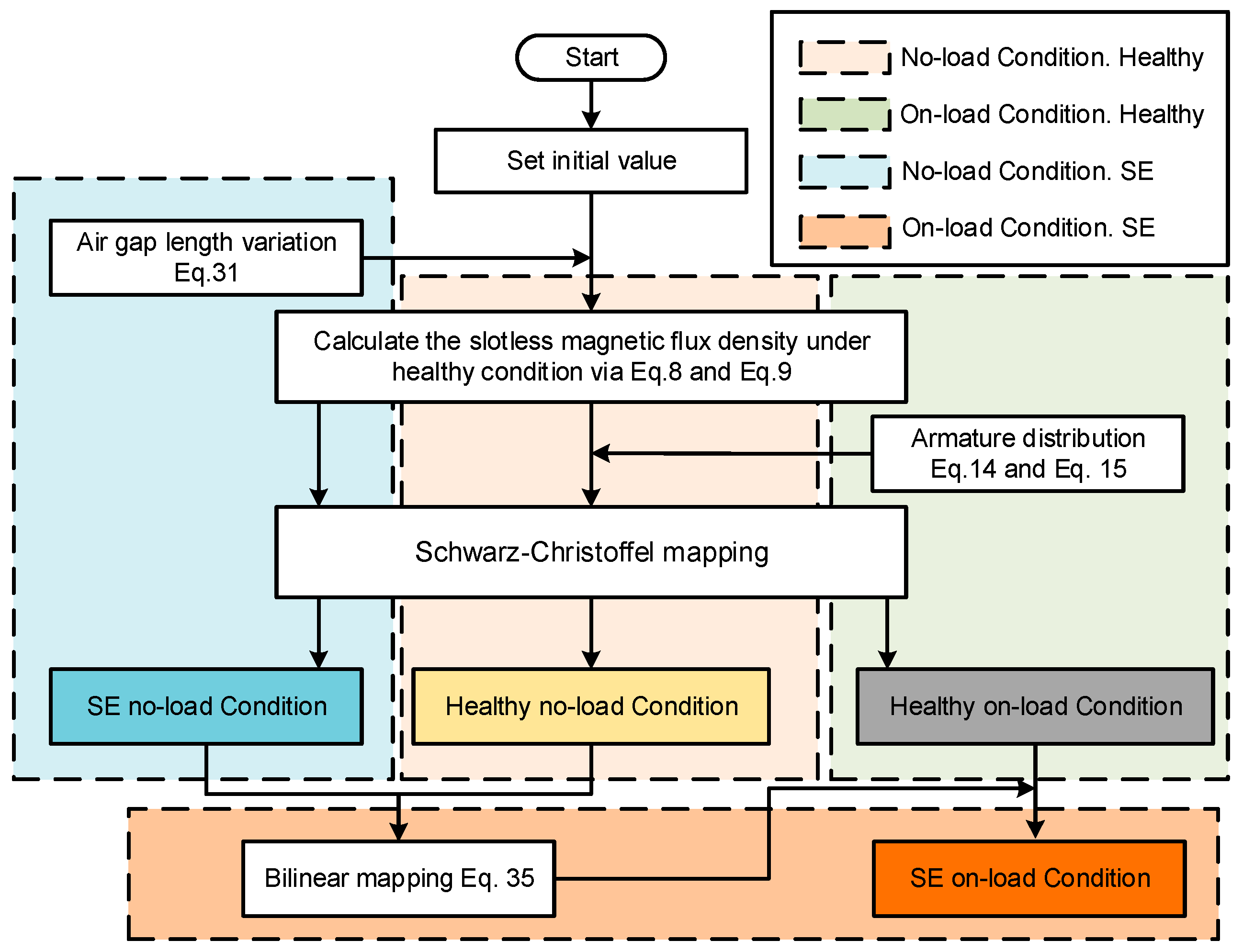
3. Calculation of the Magnetic Field

In this paper, the Quasi-3D-method is adopted in the analytical model. The machine is divided into a certain number of layers. Thus, an axial machine could be considered as a combination of several individual linear machines, which allows separate analysis of each plane. One 2D model developed in 2D polar coordinates is shown in Figure 1d and the average radius of a particular ith layer is given by:
R a v e , i = R i + R o R i 2 n s ( 2 i 1 )
where ns is the number of slices.
To improve the accuracy of the results, six slices are considered to calculate the healthy and fault conditions in this paper. The processes of quasi 3D method and two poles of a 2D model in Cartesian coordinates are illustrated in Figure 1b–d.
As for the magnetic flux calculation of air gap, the same approach in [20] is used to calculate the magnetic induction in the air gap caused by the magnets and the armature current. Moreover, to take the slot effect into account, the SC mapping [21] is adopted.
By applying Maxwell’s equations on selected slice and by summing the air gap flux caused by the armature current and magnets, the flux distribution can be obtained. The following assumptions are made during calculations in order to reduce the complexity of the computations:
(1)
The magnetic material has a uniform magnetization and the relative recoil permeability μr is constant and has a value close to unity such as in NdFeB materials.
(2)
For the computation of armature reaction field, the magnet regions are regarded as free space.
(3)
Magnetic saturation is absent and the rotor iron cores have infinite magnetic permeability.
(4)
Eddy current effects are neglected, which avoids the need for the complex eddy current field formulation.

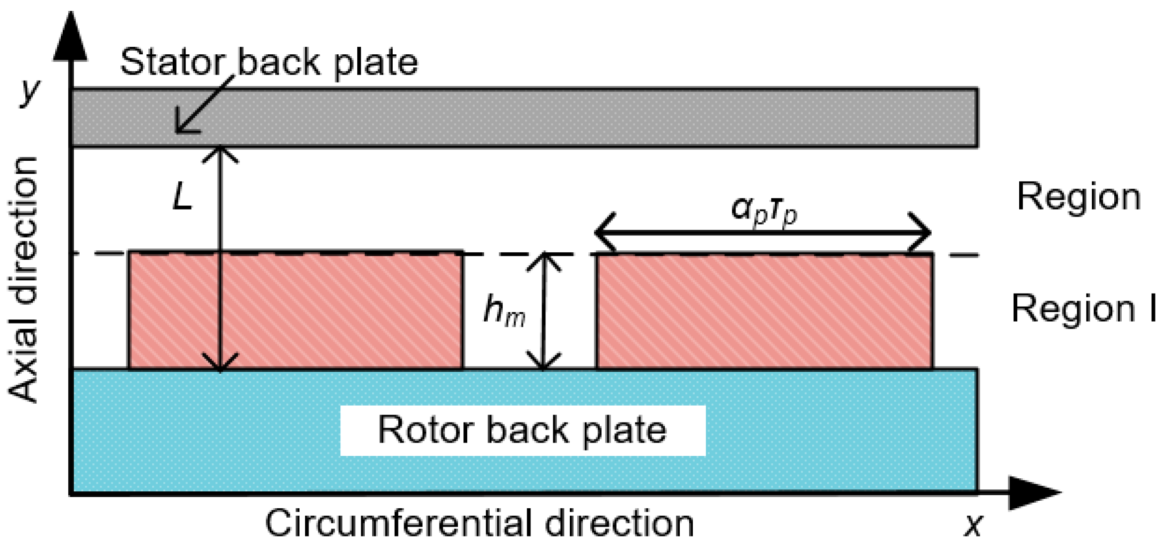
3.1. Model of Permanent Magnets (PMs)

For NdFeB, the magnetic induction in the PMs is written as:
B = B r + μ r e c H = μ 0 M r + μ r e c H
where μrec = μ0 μr is the recoil permeability.
As shown in Figure 2, the magnetization vector is assumed to be along the axial direction and may be described by Fourier series containing only cosine terms:
M y ( x ) = n = 1 , 3 , 5... M n cos ( n π x τ p )
where τp is pole pitch in circumferential direction and αp is the ratio of magnet pole arc to pole pitch, hm is axial thickness of magnets, L is the axial distance between rotor and back plates and Mn is shown as follows:
M n = 4 B r n π μ 0 sin ( n π α p 2 )
For a PM machine with linear demagnetization characteristic, the scalar magnetic potentials ( φ ) in both the air space and the PMs are governed by Laplace’s equation when the rectangular coordinate system is adopted [21].
2 φ x 2 + 2 φ y 2 = 0
The components of magnetic strength are related to φ by:
H x = φ x H y = φ y
The following boundary conditions are applied to solution of Equation (5):
{ H x I ( x , y ) | y = L = 0 H x I I ( x , y ) | y = 0 = 0 { B y I ( x , y ) | y = h m = B y I I ( x , y ) | y = h m H x I ( x , y ) | y = h m = H x I I ( x , y ) | y = h m
By applying the previous boundary conditions, the axial and circumferential flux density (By and Bx respectively) in region I and II are solved. For region I (the air space):
B x I = μ 0 H x I = μ 0 M n n = 1 , 3 , 5 , ... sinh ( n π h m / τ p ) Δ × sinh { n π ( L y ) τ p } sin ( n π x τ p )
B y I = μ 0 H y I = μ 0 M n n = 1 , 3 , 5 , ... sinh ( n π h m / τ p ) Δ × cosh { n π ( L y ) τ p } cos ( n π x τ p )
where:
Δ = μ r cosh ( n π h m τ p ) sin { n π ( L h m ) τ p } + cos { n π ( L h m ) τ p } sinh ( n π h m τ p )

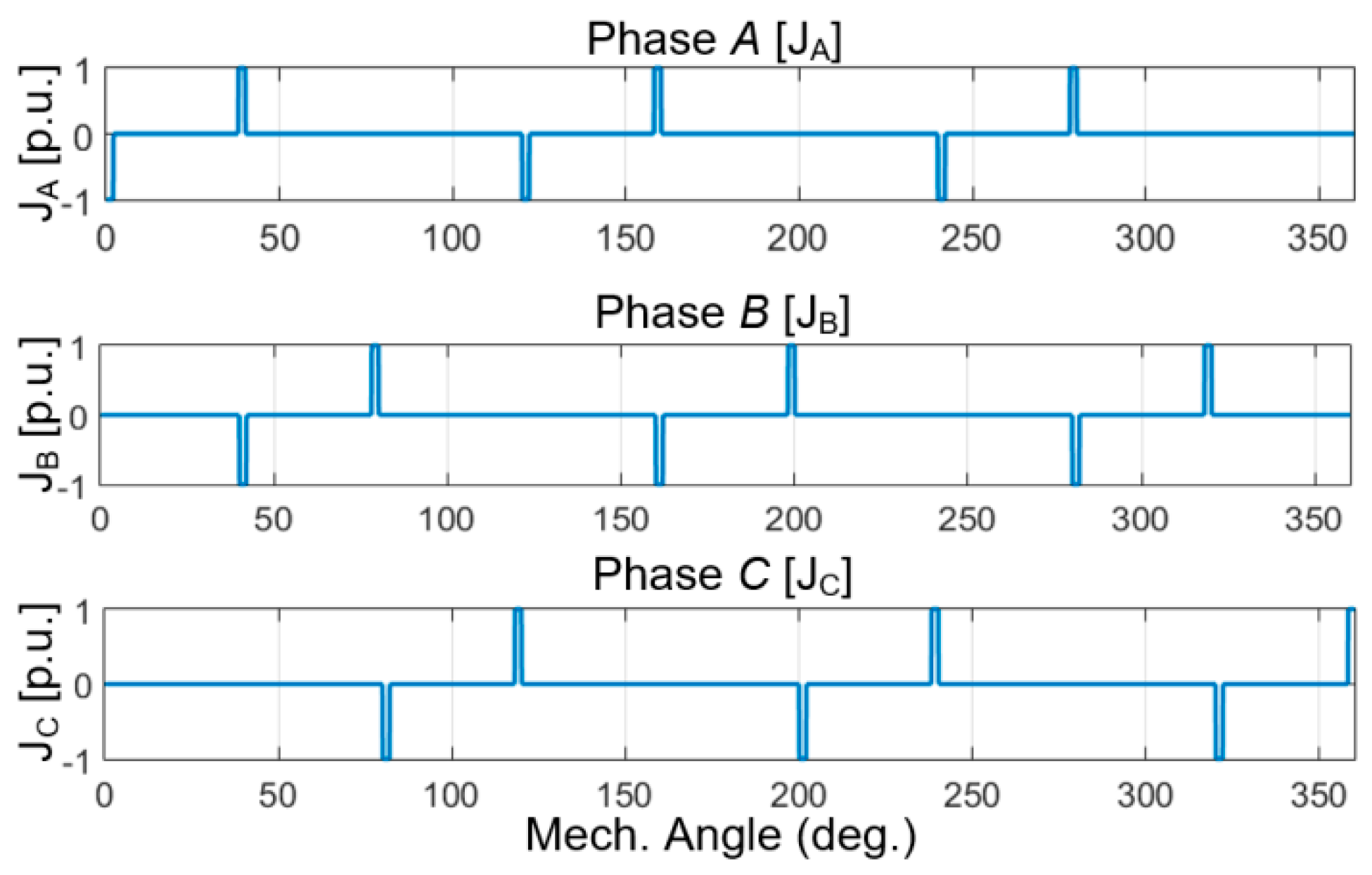
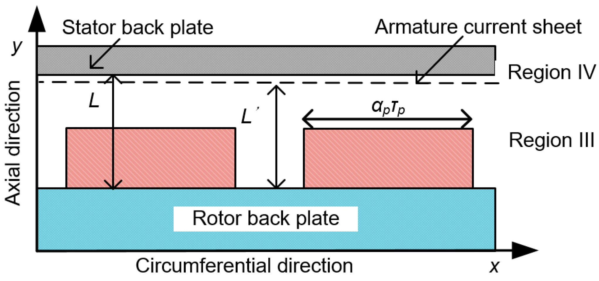
3.2. Model of Armature Reaction Current

Taking into account the armature winding current effect, the fractional slot windings are regarded as thin wires. The current density J can be obtained by multiplying the value of current sheet distribution of each phase shown in Figure 3, and dividing by the thickness of slot opening tso as follows:
J = ( J A I A sin ( ω t ) + J B I B sin ( ω t 2 π 3 ) + J C I C sin ( ω t + 2 π 3 ) ) / t s o
The current sheet spatial distribution of slots in the stator in per unit (JA, JB and JC) of each phase is plotted in Figure 3 [21].
Afterwards, the current density J is expressed by Fourier series to obtain the spatial distribution of the current, which could be derived as:
J = n = 1 , 2 , 3 ( A n cos ( n π x p τ p ) + B n sin ( n π x p τ p ) )
where An and Bn are the coefficients obtained from Fourier series.
As shown in Figure 4, the scalar magnetic potentials φ due to the current also can be described by Laplace’s equation. To solve the equation, the following boundary conditions are applied:
{ H x I I I ( x , y ) | y = 0 = 0 H x I V ( x , y ) | y = L = 0 { H x I I I ( x , y ) | y = L H x I I I ( x , y ) | y = L = J H y I I I ( x , y ) | y = L = H y I V ( x , y ) | y = L
where L′ is the axial position of a typical armature winding current sheet as shown in Figure 4.
The PMs are physically located in the lower region III and the armature current sheet is very close to the stator back plate. The result in region III will be:
B x I I I = n = 1 , 3 , 5 , ... Δ sinh ( n π y p τ p ) ( A n cos ( n π x p τ p ) + B n sin ( n π x p τ p ) )
B y I I I = n = 1 , 3 , 5 , ... Δ cosh ( n π y p τ p ) ( A n sin ( n π x p τ p ) B n cos ( n π x p τ p ) )
where:
Δ = μ 0 cosh ( ( n π / p τ p ) ( L L ) ) sinh ( n π L / p τ p )

3.3. Model of Stator Slotting

The effect of stator slotting can be linked to the previous flux density by defining a vector potential (λ) in each slot, the axial and circumferential components of flux density can be written in the form [18]:
B Z = B T λ * = ( B y + j B x ) ( R e ( λ ) + j I m ( λ ) )
To this aim, the CM method is used to calculate the λ by considering the slot effect in electrical machines, but this method has a defect mentioned above. The numerical SC mapping and its Matlab SC Toolbox could draw the real slot shape [22]:
λ = λ y + j λ x
where λ0 is the slotless air gap complex permeance in the T-plane, λx and λy are the circumferential and axial components of the complex relative air gap permeance in the original Z-plane. Furthermore, K, T, Z and S represent the K-plane, T-plane, Z-plane and S-plane, respectively.
It should be noticed that logarithmic mapping is used for the axial flux electric machine to convert the circular geometry in the S-plane to the Z-plane. However, the AFPM machines in the quasi 3D model (Figure 1) can be regarded as linear permanent magnet machines presented by the Z-plane. Hence, the SC mapping only transforms Z-plane to T-plane. However, in order to calculate the relative air gap permeance via Hague’s solution, the complex K plane is introduced in this paper. Thus, the vector potential can be deduced as:
λ = K T T Z 1 λ 0
The SC transformation in this step maps one canonical domain (e.g., a rectangle, disk, bi-infinite strip, or the upper (lower) half-plane) into the interior (exterior) of the corresponding polygon. This transformation is defined as follows:
Z = f ( T ) = A k = 1 n 1 ( t t k ) α t π d t + C
where A and C are unknown complex constants, n is the number of polygon corners with interior angle αt, t1, …, tk are the points in the canonical domain (in the T-plane) corresponding to the polygon corners.
The analytical solution of Equation (20) is very difficult for geometries with more than three vertices [22], therefore, the SC Toolbox provides a numerical solution by a library of command-line functions which could be seen in [19]. In this paper, the rectangle domain (T-plane) is created by calling f = correctmap (p, alpha), p is the point and alpha is the corresponding angle as shown in Figure 5.
The next step aims to map the interior of annular domain in K-plane to rectangular domain in T-plane. This mapping can be calculated analytically:
T ( t ) = j ( log ( K ( k ) ) Δ x 2 π + Δ y 2 j Δ x 2 )
With the determinate rectangular domain vertices by calling vt = evalinv (f, vz), the length (Δx) and width (Δy) of the T-plane could be calculated.
Finally, Hague solution for magnetic field in an annular domain could be used, and the final equation which maps the field solution from the K-plane to Z-plane is given as Equation (19), where T / Z can be obtained in SC Toolbox by calling evaldiff (f, Z) and:
K T = j Δ x 2 π 1 T
Afterwards, the magnetic flux density at slotted air gap field could be calculated by Equation (17).

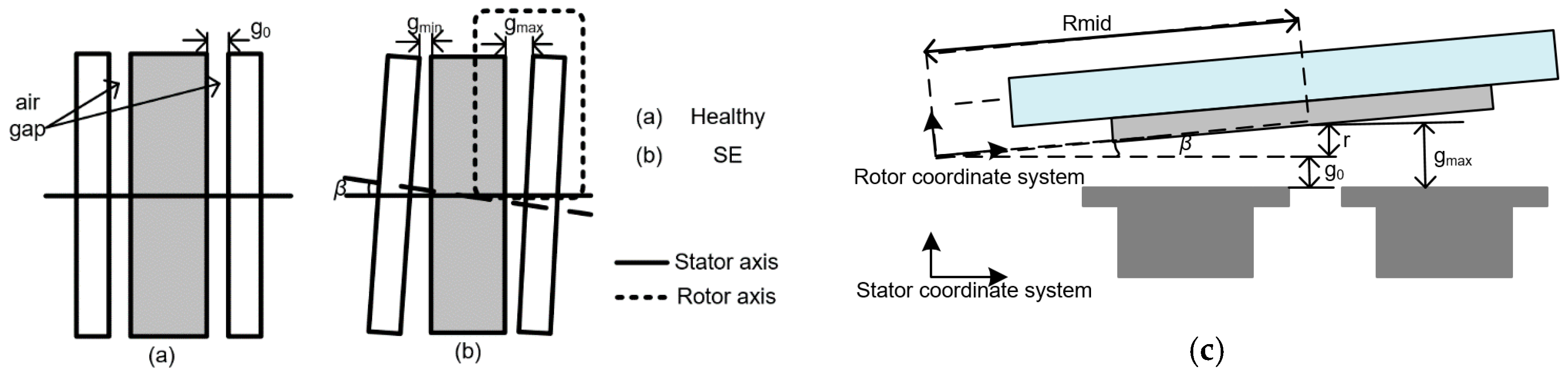
3.4. Model of Static Eccentricity

SE is a misalignment condition of stator and rotor axis, thus, the rotor axis is deflected from that of the stator which causes a non-uniform air gap. In a healthy state (Figure 6a), the air gap length g0 is uniform along the circumferential direction. However, with the occurrence of SE (Figure 6b,c), the rotor shaft experiences a deflection and the symmetry of the rotor deviates from that of the stator by an angle β. The air gap varies from small to large around the circumferential of the stator but the relative position does not vary with time. In other words, in the case of SE the position of the minimum air gap length is fixed in space.
The first step in modeling the eccentricity is to evaluate the air gap length in SE condition [23], the SE factor can be defined as:
S E F = r g 0 × 100 %
The air-gap length at mean radius Rmid can be written as follows:
g m ( θ ) = g 0 ( 1 S E F cos ( θ γ 0 ) )
where θ is the stator position measured from a reference point (γ0) of the minimal air gap. According to Figure 6b, the air gap length in all positions can be understood as:
g ( R , θ ) = g m ( θ ) g ( R , θ )
where g’ is the air gap deviation at the Rmid:
g ( R , θ ) = ( R R m i d ) sin β cos ( θ γ 0 )
Therefore, the air gap length in all positions can be written as follows:
g ( R , θ ) = g 0 ( 1 R R m i d S E F cos ( θ γ 0 ) )
Because of the high ratio of machine diameter to length in the AFPMs, 40% SEF means that the maximum declined distance of rotor plate is 1.2 mm in this case, which is already a significant value compared to the air gap length of 3 mm.
In this paper, as quasi-2D model processed in Figure 1, the minimal air gap happens at γ0 = 0 rad and the maximum air gap at θ= π rad. Finally, the air gap length can be deduced as follows:
g ( R , θ ) = g 0 ( 1 R R m i d S E F cos ( π x p τ p ) )

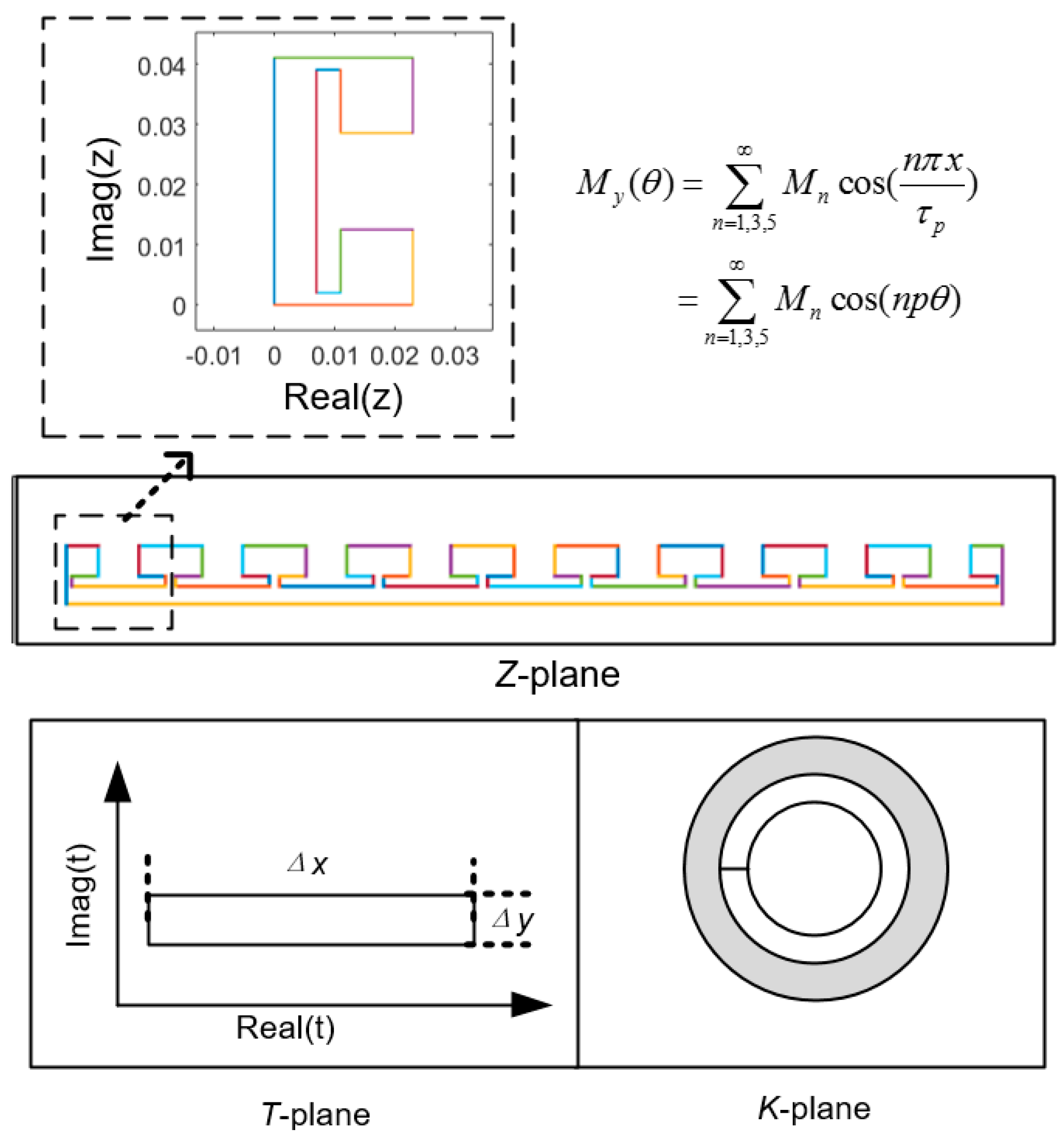
3.5. Bilinear Mapping

Bilinear mapping [24] is a particular mapping method which is used for the treatment of the boundaries which are circular but eccentric or intersecting. The purpose of this process is to map the pair of eccentric circles (E-plane) into a pair of concentric circles (S-plane). After mapping E-plane to the S-plane, the following mapping could be done by previous study. The general form of this CM can be defined as:
E ( s ) = 1 s + C K
H S = H E ( E S ) *
where parameters C and K are determined by the rotor and stator radii and the magnitude of eccentricity.
Markovic used this method to calculate a non-salient motor under SE. Bilinear maps preserve the scalar magnetic potential but they cannot conserve the vector field potential (Ωv) because flux density in concentric plane is coupled with the coordinate system. Since vector field potential calculation is complex and it is very difficult to estimate the scale factor required to map magnetic field into desired eccentric domain, in this paper, the following form is used to convert the air gap flux density of concentric AFPM motor in Z-plane to the eccentric model in E-plane [25]:
B E = B Z λ e
where λe is the relative permeance function due to the effect of SE and can be defined as:
λ e ( r , θ ) = B e c c ( r , θ ) / B n o e c c ( r , θ )
The flux density in the slotless air gap with eccentricity (Becc) and without eccentricity (Bno-ecc) can be estimated by modifying the air gap length in Equation (9).
The calculation processes can be seen in Figure 7.

4. Simulation Verification

To validate the analytical model, an AFPMM with nine slots and six poles has been studied. The basic parameters are shown in Table 1. The air gap flux distribution is one of the most important characteristics in electrical machines because any change of this feature would affect the performance of motor. In this section, as the first step of investigation, the air gap flux density under healthy condition is presented. The results of the analytical model are compared with the results calculated by FE model. As the second step, the flux density under SE at the same conditions is also compared with the FE results. Moreover, the effect of eccentricity on air gap flux of AFPM will be discussed in the final step.

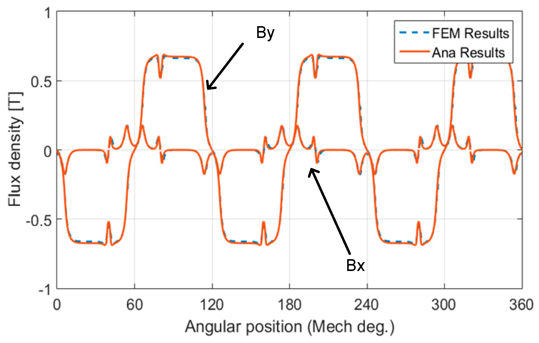
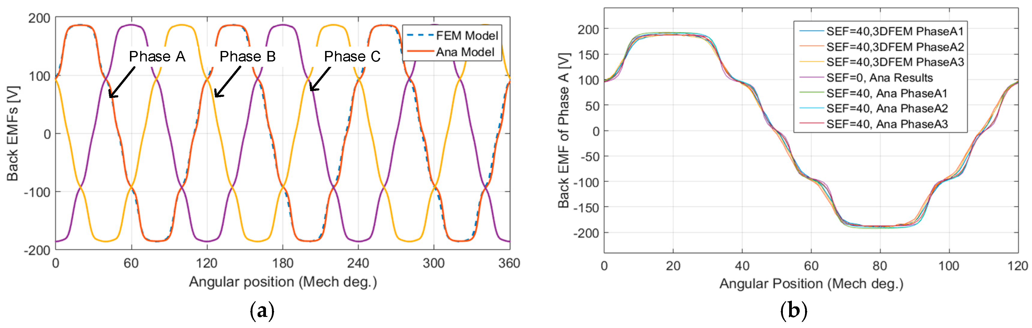
4.1. Air Gap Flux under Healthy Condition

The axial and circumferential components of complex relative permeance in the middle of air gap are shown in Figure 8. It shows that, under healthy condition, the complex relative air gap permeance is periodic for each slot pitch.
With Equation (17), the axial and circumferential components of the flux density in the slotted air gap are given by:
B Z y = B y λ y + B x λ x
B Z x = B x λ y B y λ x
The axial and circumferential flux density at the center of air gap under no-load condition are shown in Figure 9. Figure 10 shows the flux density at the rated current (10 A), 20 krpm. The figures show that the analytical model is in a very good agreement with the FE model.

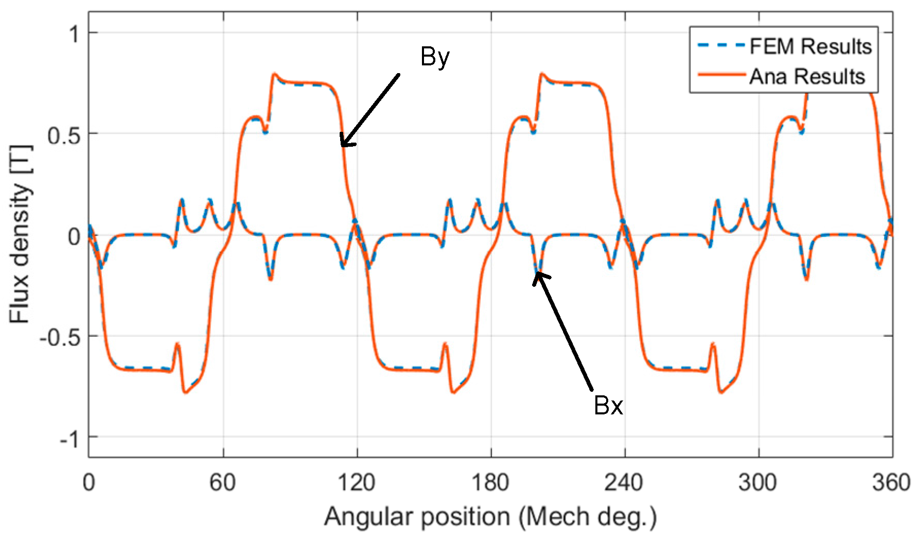
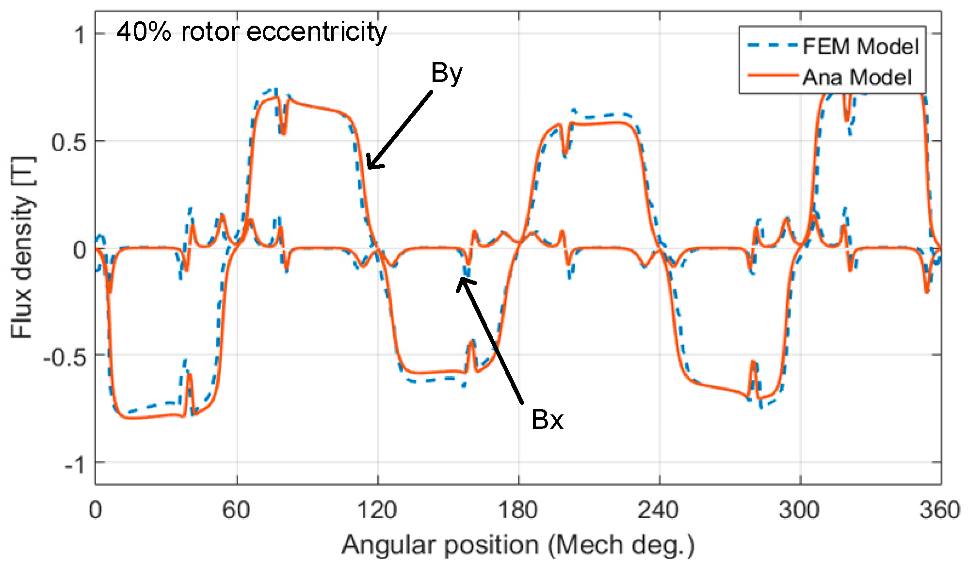
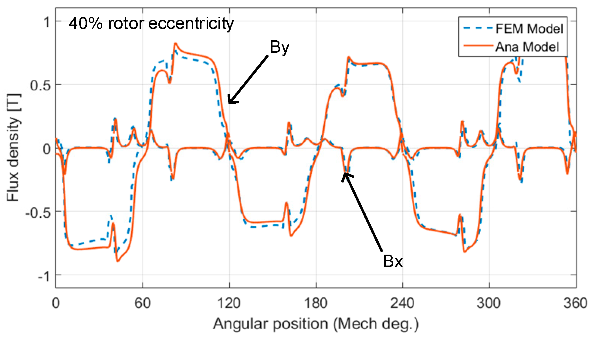
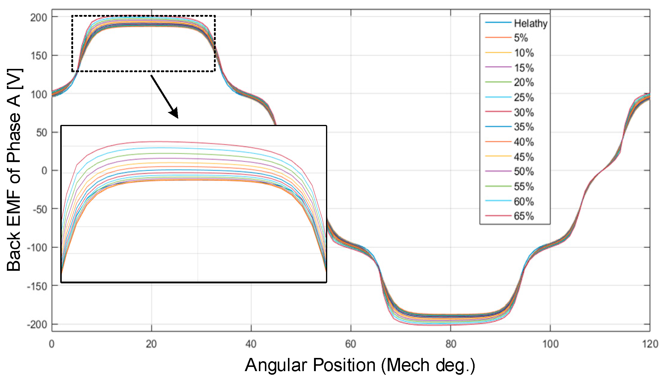
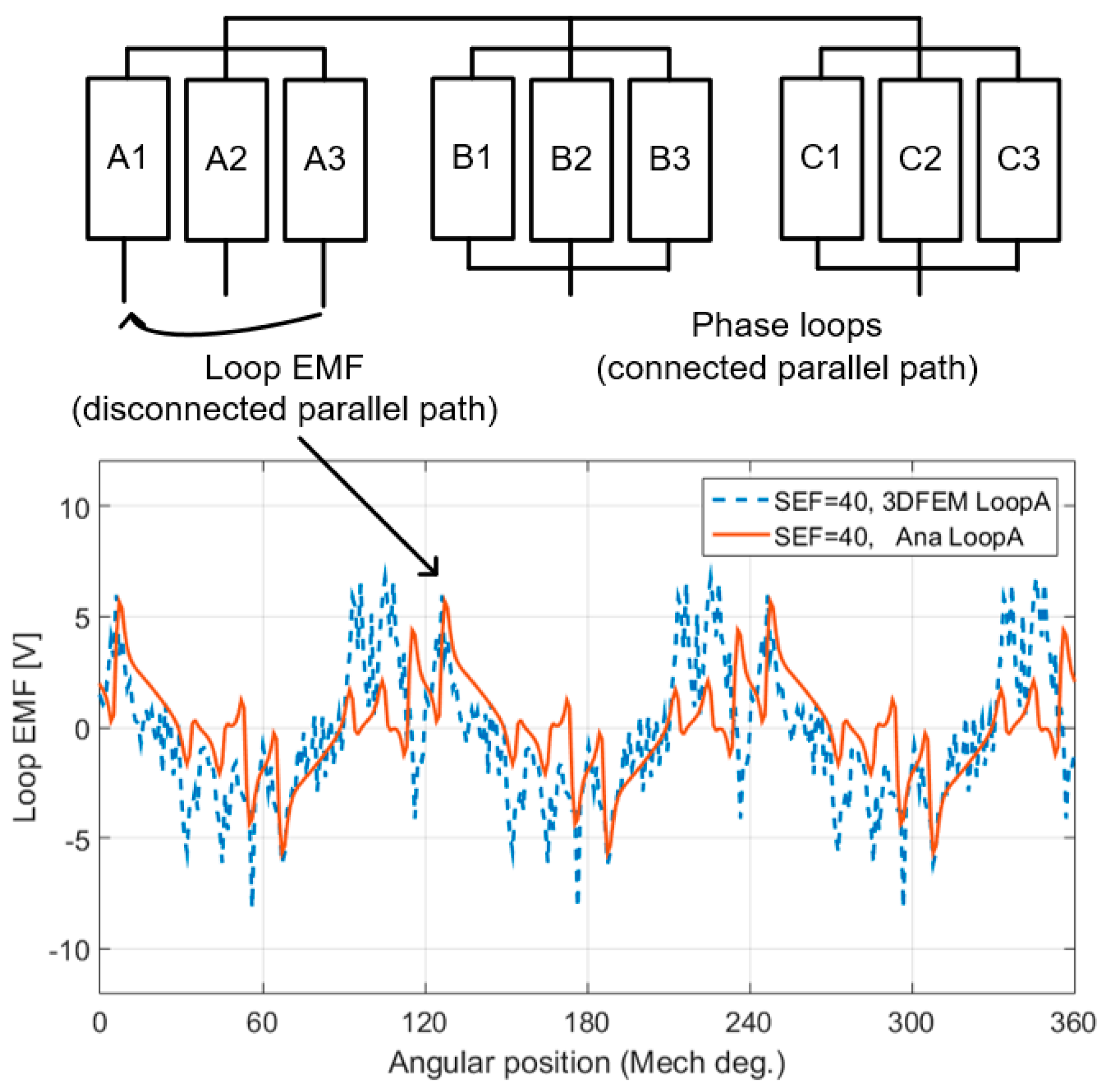
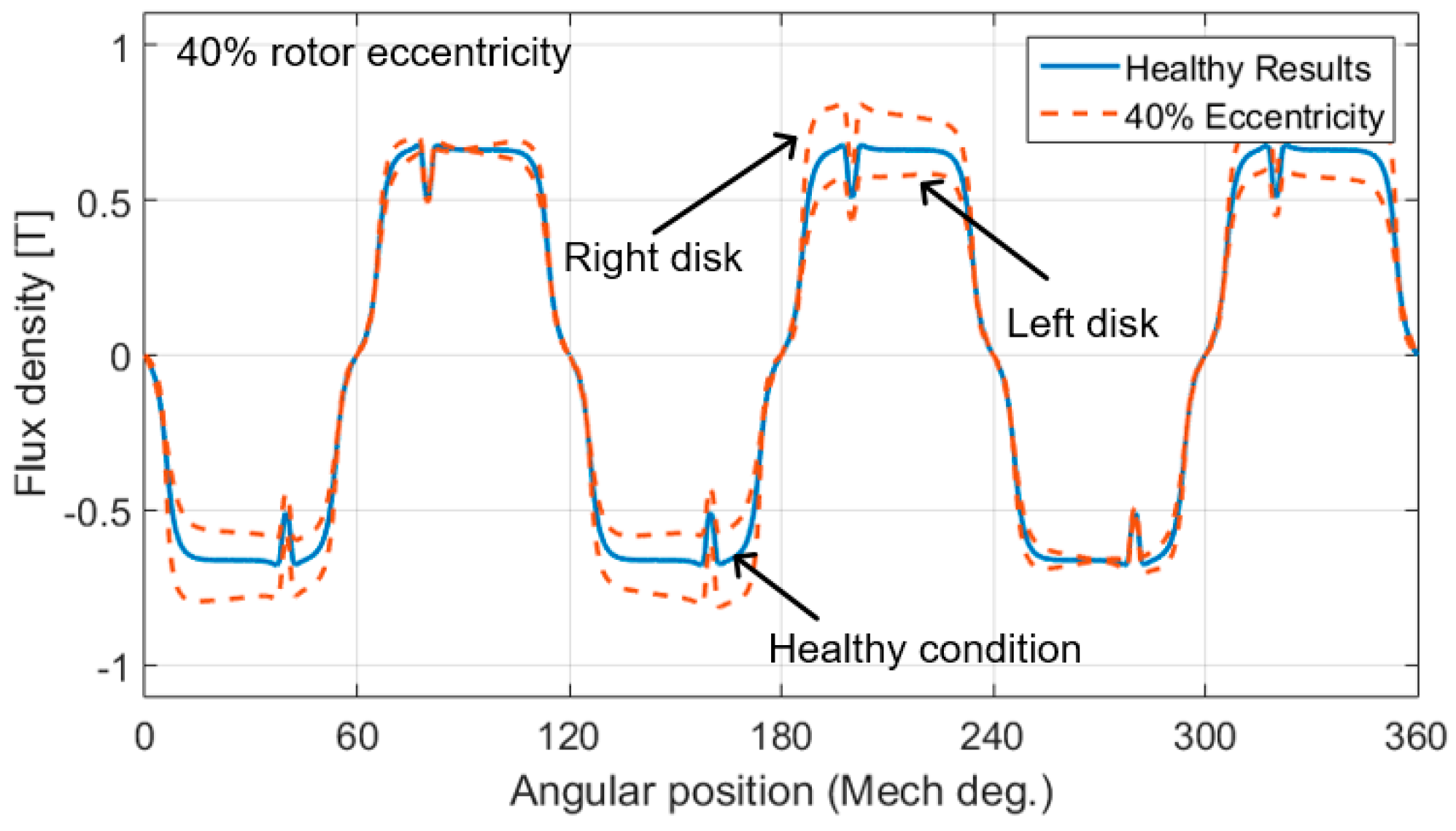
4.2. Air Gap Flux Density under SE Condition

In order to verify the SE model, the rotor of AFPM is assumed with 40% eccentricity. It is shown in previous section that the slotless flux density caused by PMs under SE and healthy condition could be solved analytically, thus, the relative permeance function of SE can be determined. The FE model is represented by two rotor disc to ensure the real flux distribution. The 3D FE model and its grid could be seen in Figure 11. The rotor axis is set as shown in Figure 6a.
The axial and circumferential components of one side rotor disk with 40% eccentricity under no-load and rated load condition conditions are shown in Figure 12 and Figure 13, respectively. It can be seen that the axial and circumferential components of the flux density between the FE model and analytical method do not agree well due to the interaction between the circumferential and axial flux density, but the error still remains in a reasonable range. Overall, the proposed method in this paper is an effective way to investigate the eccentric influence of AFPM.

5. Results and Discussion

In this section, some important machine characteristics, e.g., back-EMF and torque, will be presented and compared. Since these characteristics under different SE conditions only differ in magnitude, the 40% eccentricity is chosen to carry out the analysis.
As shown in Figure 14, the flux passes from one rotor disc and enters the other rotor disc. Therefore, the coils are assumed to be symmetrical with respect to the stator teeth axis. Hence, both rotors contribute with the same amount of magnetic flux (ϕLkRk). Therefore, the flux linkage of the kth tooth coil with Nc turns is simply given by:
ψ k = N c ( φ L k + φ R k ) / 2

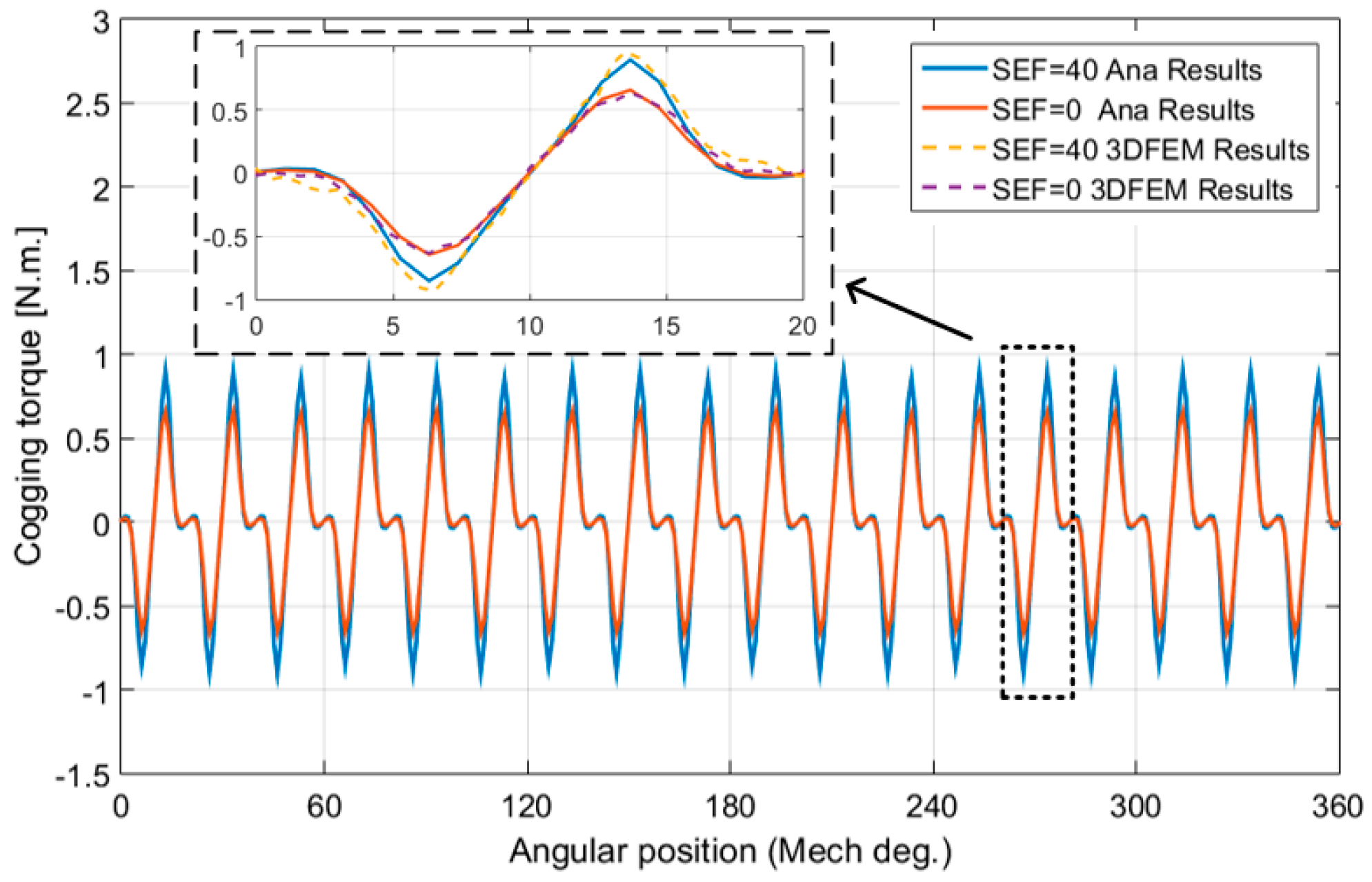
5.1. Machine Main Characteristics under No Load Condition

The no-load air gap total flux density under healthy condition compared with 40% eccentricity condition, the analytical results are shown in Figure 15.
Comparing with the healthy conditions, it can be seen that the flux density near minimum air gap has increased but the flux density near maximum air gap has decreased. This is owing to the partly increased yet partly decreased air gap length around circumferential direction.
The back EMF and cogging torque are also important for PM machines. For this purpose, the rotor movement should be modeled to calculate these parameters. The back EMF waveform of the AFPM can be calculated from the axial component of the no-load flux density distribution (By) with the knowledge of the armature winding distribution. The voltage induced in a single coil in each layers of quasi-3D method can be calculated as:
E c , i = N c d ψ c , i d t
where Ψc,i is the flux linkage of the coil in ith layer and is equal to the integral of the air gap flux density distribution across one coil pitch, as given by:
ψ c , i = R a v e , i ( R o R i ) n s θ 0 θ 0 + θ c B y , i d θ
where θ0 is the coil starting side angle from origin and θc is the angle of coil pitch, and By,i is the axial component of flux density in ith layer.
The back-EMF per phase is calculated in all coils with the phase winding connected in parallel. For phase A, according to the coils arrangement shown in Figure 3, the back-EMF in ith layer EA,i is given by:
E A , i = N c R a v e , i ( R o R i ) n s d ψ c , i d t
And based on the quasi-3-D consumption, the back EMF for the whole machine is calculated as:
E A = i n s E A , i
The back-EMF of the prototype AFPM with and without SE condition obtained from both FE and SC methods are compared in Figure 16.
It can be seen that in healthy condition, the induced voltage of three coils have the same shape and amplitude. However, monitoring back EMF is not an effective approach to detect eccentric fault in double rotor AFPMs since the back EMF is not affected by eccentricity sufficiently in SE condition. Eccentricity increases the air gap, but on the other hand, the air gap length of corresponding position of the other rotor is decreased. These two effects seem to compensate each other, given the same results.
The back EMFs and its fast Fourier transform (FFT) under SE condition varies from 0% to 65% is shown in Figure 17 and Figure 18 respectively. When the SE factor is increasing, the amplitude of back EMFs is slightly increasing. Moreover, the SE has a strong impact on the first order of FFT.
In the case of SE, the following differential flux linkages act on the phase loops [26], in this paper, phase A is disconnected the parallel path (shown in Figure 16) and:
ψ d l = ψ l I ψ l I I
where ψ l I and ψ l I I are magnetic flux linkages of two disconnected parallel paths of phase A.
By time deriving, the no-load loop EMF follows:
E d l = d ψ d l / d t
Thus, monitoring loop EMF could be a practical approach to detect defects of AFPMs. Figure 19 shows the distribution of phase A loop EMF during one complete rotor revolution at rated speed. It can be seen that the loop EMF fluctuates at each position.
The cogging torque is another important parameter for PM machines which occurs in slotted AFPM machine due to the interaction between the PM magnetic field and the varying air gap permeance.
By assuming negligible saturation, the cogging torque is independent of armature currents and is created only by the PM magnetic field. The period of the cogging torque waveform is calculated as follows:
Cogging torque period = 2π/LCM (Qs, 2p)
where LCM (Qs, 2p) is the least common multiple of the stator slot number and the rotor pole number.
The cogging torque is calculated by the changing rate of total air gap co-energy including the region of PMs [27]:
T c o g = W θ = θ ( τ B t t o t a l 2 d τ )
It should be noted that the AFPM machine in this paper has two rotor disks, which means that both rotors contribute to the cogging torque. Thus, the cogging torque of each disk should be superimposed. The cogging torque waveforms obtained under healthy and SE condition are compared in Figure 20. Comparing with the results obtained from FE model, we can see that the results obtained by analytical model do not agree well, this is mainly due to the subtraction in Equation (40), but the trend of analytical model is still in accordance with that of FE model.
In order to validate the results, 3D FEM calculation is also depicted, which shows a good agreement with analytical simulations. From the simulation results and comparisons, the cogging torque of each disk has the same shape and amplitude, but under SE condition, the cogging torque is increased.

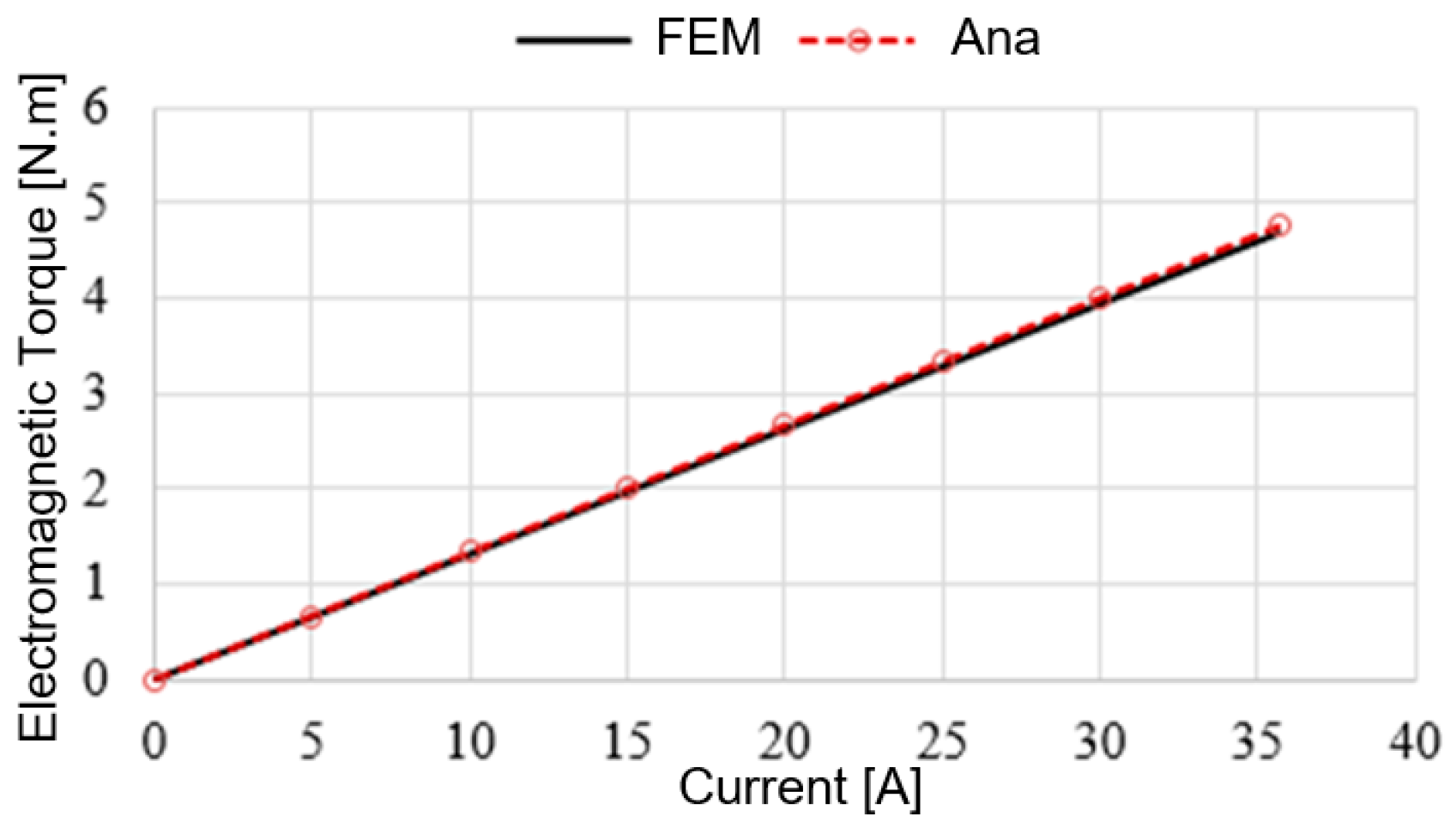
5.2. Machine Main Characteristics under on Load Condition

The output torque is comprised of EM and cogging torque. Neglecting saturation, currents in each phase are updated according to rotor position. The electromagnetic torque for each layer could be calculated by integrating Maxwell stress tensor near the center of the air gap:
T e m , i = R a v e , i 2 ( R o R i ) μ 0 n s 0 2 π B arm x , i B a r m y , i d θ
The electromagnetic torque of machine is obtained as:
T e m = i = 1 n s T e m , i
Also, the average electromagnetic torque can be simply calculated from
T e m = 3 2 p N c k w ϕ f I
where kw is the winding factor,φf is the magnetic flux excited by the permanent magnet per pole and I is the stator current. From pervious study, the magnetic flux of each phase can be compensated by the right and left magnetic flux, thus, SE does not have significant effects on the EM torque. This also can be proved in Equation (46).
As shown in Figure 21, the results of the proposed method are in good agreement with the simulation results of 3D-FE model.

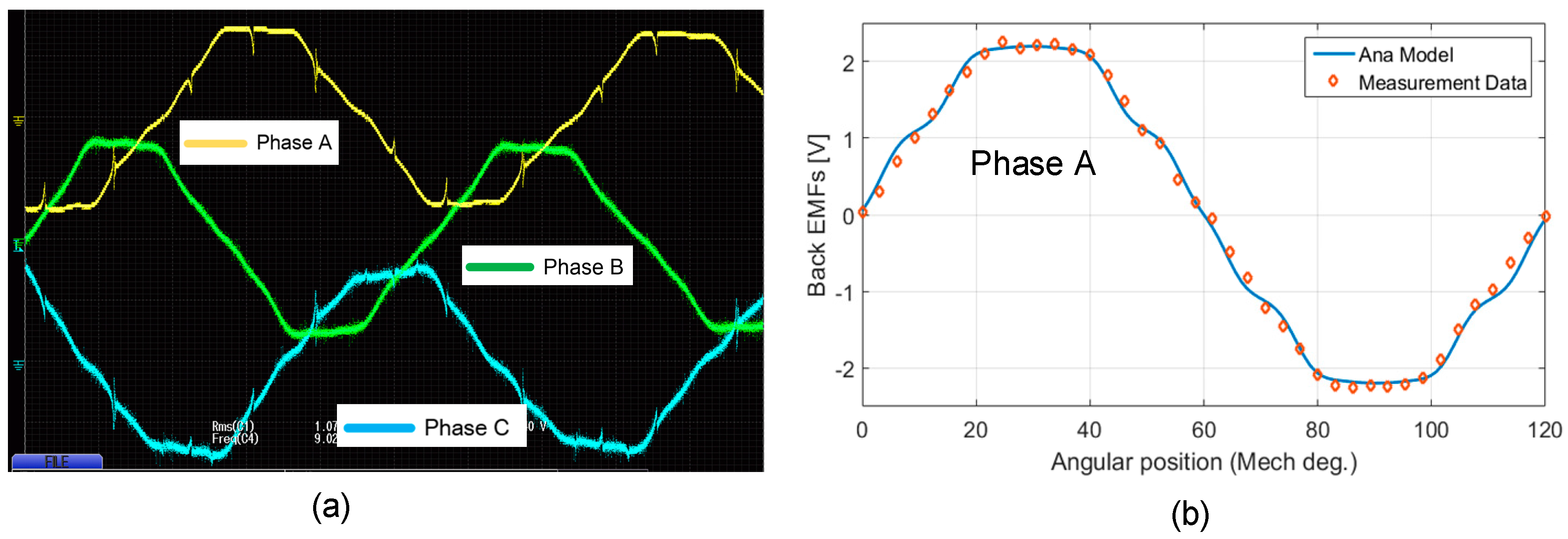
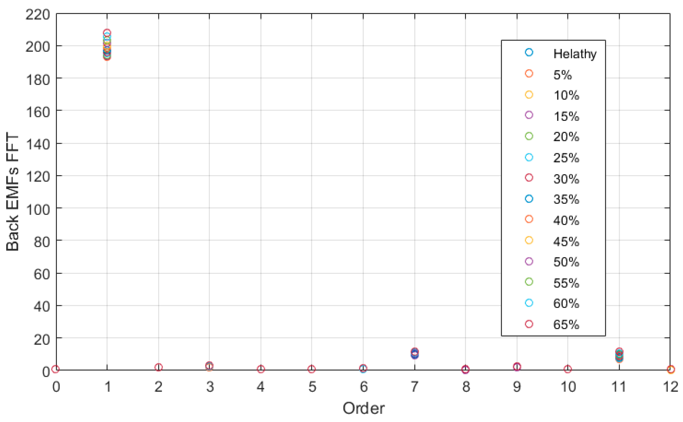
6. Experimental Results

The double rotor AFPM in Table 1 is the prototype machine investigated in this paper, as shown in Figure 22a,b. The experimental set-up and devices are presented in Figure 22c. The AFPM motor is driven by a frequency converter shown in Figure 22c to test its motor performance, and the no-load parameters.
The back EMF is measured by a driving motor via a belt and the drive speed is 300 rpm, the measured back EMF is shown in Figure 23. The analytical model provides good correspondence with the experimental results shown in Figure 16. Table 2 shows the back EMF coefficient obtained by analytical model, FE model and experiment, respectively. However, there is a slight error between the analytical results and the measured value which is mainly caused by the assembly process.
In terms of the computational time, the analytical model requires only 206 s to obtain the cogging torque and electromagnetic torque with one mechanical cycle for SE condition. The 3D FE model, on the other hand, requires almost 27 h to compute the performance in one electrical cycle. Although the analytical method shows a slight error compared to the experimental result, it is still acceptable and thus, can be regarded as a meaningful approach which could save time and achieve a satisfying result. Moreover, the analytical model could also be used for further calculation, e.g., optimization.

7. Conclusions

In this paper an approach for modeling double rotor AFPM with SE has been presented. To take into account the intrinsic 3D nature of the AFPM machine, a quasi-3D method is used. The magnetic field, cogging torque and output torque of AFPM machine under healthy and 40% eccentricity conditions are quickly calculated with great accuracy compared to the 3D FE model and experimental results. In addition, it can be found that the eccentricity plays no effects on the back EMF and the electromagnetic torque. However, the cogging torque increases with SE. In addition, this paper makes a remarkable contribution to the computational time savings while maintaining as much the high accuracy the FE model can provide. Finally, an experimental validation has been carried out to verify the accuracy of the simulation results obtained by the proposed method.

Acknowledgments

This work was supported in part by Natural Science Foundation of China (Project Number 51377019), the Scientific and Technological Innovation Program of Jiangsu Province (Project Number BY201412715), and the Qing Lan Project.

Author Contributions

Each of the authors contributes on performing experiments and writing articles. Baocheng Guo and Ahmed Hemeida are the main authors of this manuscript and this work was conducted under advisement of Yunkai Huang and Peter Sergeant. All authors revised and approved the publication.

Conflicts of Interest

The authors declare no conflict of interest.

References

  1. Aydin, M.; Huang, S.; Lipo, T.A. Axial Flux Permanent Magnet Disc Machines: A Review; University of Wisconsin-Madison: Madison, WI, USA, 2004. [Google Scholar]
  2. Yang, Y.P.; Shih, G.Y. Optimal Design of an Axial-Flux Permanent-Magnet Motor for an Electric Vehicle Based on Driving Scenarios. Energies 2016, 9, 285. [Google Scholar] [CrossRef]
  3. Hua, W.; Zhou, L.K. Investigation of a Co-Axial Dual-Mechanical Ports Flux-Switching Permanent Magnet Machine for Hybrid Electric Vehicles. Energies 2015, 8, 14361–14379. [Google Scholar] [CrossRef]
  4. Bai, C.-J.; Wang, W.-C.; Chen, P.-W.; Chong, W.-T. System Integration of the Horizontal-Axis Wind Turbine: The Design of Turbine Blades with an Axial-Flux Permanent Magnet Generator. Energies 2014, 7, 7773–7793. [Google Scholar] [CrossRef]
  5. Nguyen, T.D.; Tseng, K.-J.; Zhang, S.; Nguyen, T.D. A Novel Axial Flux Permanent-Magnet Machine for Flywheel Energy Storage System: Design and Analysis. IEEE Trans. Ind. Electron. 2011, 58, 3784–3794. [Google Scholar] [CrossRef]
  6. Mirimani, S.M.; Vahedi, A.; Marignetti, F. Effect of Inclined Static Eccentricity Fault in Single Stator-Single Rotor Axial Flux Permanent Magnet Machines. IEEE Trans. Magn. 2012, 48, 143–149. [Google Scholar] [CrossRef]
  7. Thiele, M.; Heins, G.; Patterson, D. Identifying manufacturing induced rotor and stator misalignment in brushless permanent magnet motors. In Proceedings of the 2014 International Conference on Electrical Machines (ICEM), Berlin, Germany, 2–5 September 2014; pp. 2728–2733.
  8. Thiele, M.; Heins, G. Computationally Efficient Method for Identifying Manufacturing Induced Rotor and Stator Misalignment in Permanent Magnet Brushless Machines. IEEE Trans. Ind. Appl. 2016, 52, 3033–3040. [Google Scholar] [CrossRef]
  9. Li, J.; Qu, R.; Cho, Y.-H. Effect of unbalanced and inclined air-gap in double-stator inner-rotor axial flux permanent magnet machine. In Proceedings of the 2014 International Conference on Electrical Machines (ICEM), Berlin, Germany, 2–5 September 2014; pp. 502–508.
  10. Bellini, A.; Filippetti, F.; Tassoni, C.; Capolino, G.A. Advances in Diagnostic Techniques for Induction Machines. IEEE Trans. Ind. Electron. 2008, 55, 4109–4126. [Google Scholar] [CrossRef]
  11. Marignetti, F.; Vahedi, A.; Mirimani, S.M. An Analytical Approach to Eccentricity in Axial Flux Permanent Magnet Synchronous Generators for Wind Turbines. Electr. Power Compon. Syst. 2015, 43, 1039–1250. [Google Scholar] [CrossRef]
  12. Mirimani, S.M.; Vahedi, A.; Marignetti, F.; di Stefano, R. An Online Method for Static Eccentricity Fault Detection in Axial Flux Machines. IEEE Trans. Ind. Electron. 2015, 62, 1931–1942. [Google Scholar] [CrossRef]
  13. Abbaszadeh, K.; Maroufian, S.S. Axial flux permanent magnet motor modeling using magnetic equivalent circuit. In Proceedings of the 2013 21st Iranian Conference on Electrical Engineering (ICEE), Mashhad, Iran, 14–16 May 2013.
  14. Azzouzi, J.; Barakat, G.; Dakyo, B. Quasi-3-D analytical modeling of the magnetic field of an axial flux permanent-magnet synchronous machine. IEEE Trans. Energy Convers. 2005, 20, 746–752. [Google Scholar] [CrossRef]
  15. Ajily, E.; Ardebili, M.; Abbaszadeh, K. Magnet Defect and Rotor Eccentricity Modeling in Axial-Flux Permanent-Magnet Machines via 3-D Field Reconstruction Method. IEEE Trans. Energy Convers. 2016, 31, 486–495. [Google Scholar] [CrossRef]
  16. Ajily, E.; Abbaszadeh, K.; Ardebili, M. Three-Dimensional Field Reconstruction Method for Modeling Axial Flux Permanent Magnet Machines. IEEE Trans. Energy Convers. 2015, 30, 199–207. [Google Scholar] [CrossRef]
  17. Abbaszadeh, K.; Rahimi, A. Analytical quasi 3D modeling of an axial flux PM motor with static eccentricity fault. Sci. Iran. Trans. Comput. Sci. Eng. Electr. 2015, 22, 2482. [Google Scholar]
  18. Zarko, D.; Ban, D.; Lipo, T.A. Analytical Solution for Electromagnetic Torque in Surface Permanent-Magnet Motors Using Conformal Mapping. IEEE Trans. Magn. 2009, 45, 2943–2954. [Google Scholar] [CrossRef]
  19. Žarko, D. A Systematic Approach to Optimized Design of Permanent Magnet Motors with Reduced Torque Pulsations. Ph.D. Thesis, University of Wisconsin-Madison, Madison, WI, USA, 2004. [Google Scholar]
  20. O’Connell, T.C.; Krein, P.T. A Schwarz–Christoffel-Based Analytical Method for Electric Machine Field Analysis. IEEE Trans. Energy Convers. 2009, 24, 565–577. [Google Scholar] [CrossRef]
  21. Hemeida, A.; Sergeant, P. Analytical Modeling of Surface PMSM Using a Combined Solution of Maxwell’s Equations and Magnetic Equivalent Circuit. IEEE Trans. Magn. 2014, 50, 1–13. [Google Scholar] [CrossRef]
  22. Calixto, W.P.; Alvarenga, B.; da Mota, J.C.; Brito, L.D.C.; Wu, M.; Alves, A.J.; Neto, L.M.; Antunes, C.F.R.L. Electromagnetic Problems Solving by Conformal Mapping: A Mathematical Operator for Optimization. Math. Probl. Eng. 2010, 2010, 742039. [Google Scholar] [CrossRef]
  23. Ogidi, O.O.; Barendse, P.S.; Khan, M.A. Detection of Static Eccentricities in Axial-Flux Permanent-Magnet Machines with Concentrated Windings Using Vibration Analysis. IEEE Trans. Ind. Appl. 2015, 51, 4425–4434. [Google Scholar] [CrossRef]
  24. Miroslav, M. Magnetic Field Analysis in Electric Motors Using Conformal Mapping; EPFL: Lausanne, Switzerland, 2004. [Google Scholar]
  25. Li, J.T.; Liu, Z.J.; Nay, L.H.A. Effect of Radial Magnetic Forces in Permanent Magnet Motors with Rotor Eccentricity. IEEE Trans. Magn. 2007, 43, 2525–2527. [Google Scholar] [CrossRef]
  26. Di Gerlando, A.; Foglia, G.M.; Iacchetti, M.F.; Perini, R. Evaluation of Manufacturing Dissymmetry Effects in Axial Flux Permanent-Magnet Machines: Analysis Method Based on Field Functions. IEEE Trans. Magn. 2012, 48, 1995–2008. [Google Scholar] [CrossRef]
  27. Barakat, G.; El-meslouhi, T.; Dakyo, B. Analysis of the cogging torque behavior of a two-phase axial flux permanent magnet synchronous machine. IEEE Trans. Magn. 2001, 37, 2803–2805. [Google Scholar] [CrossRef]
Figure 1. Construction of the investigated axial flux permanent magnet machine (AFPMM) (a) and the principle of quasi-3D method (bd).
Energies 09 00892 g001
Figure 2. Representation of field regions divided by magnets.
Energies 09 00892 g002
Figure 3. Current sheet spatial distribution in space of each phase in per unit for AFPM with six poles and nine stator slots.
Energies 09 00892 g003
Figure 4. Representation of field regions caused by armature reaction current sheet.
Energies 09 00892 g004
Figure 5. Schwarz-Christoffel (SC) mapping in different plane.
Energies 09 00892 g005
Figure 6. (a) Double sided topology of AFPMM machine in 2D plane; (b) Static eccentricity (SE) in AFPMs; and (c) Detailed configuration of SE.
Energies 09 00892 g006
Figure 7. Calculation processes of magnet flux density.
Energies 09 00892 g007
Figure 8. Complex relative permeance without eccentricity in the middle of air gap. (a) Axial component; and (b) Circumferential component.
Energies 09 00892 g008
Figure 9. Axial and circumferential components of permanent magnetic (PM) flux density at the center of air gap under no-load condition.
Energies 09 00892 g009
Figure 10. Axial and circumferential components of PM flux density at the center of air gap under rated load.
Energies 09 00892 g010
Figure 11. The 3D FE model and its meshing.
Energies 09 00892 g011
Figure 12. Axial and circumferential components of flux density at the air gap (l = L − 1 mm) under no-load condition.
Energies 09 00892 g012
Figure 13. Axial and circumferential components of flux density at the air gap (l = L − 1 mm) under rated-load condition.
Energies 09 00892 g013
Figure 14. Right and left magnetic flux in the tooth.
Energies 09 00892 g014
Figure 15. Total flux density comparison at the air gap under no-load condition.
Energies 09 00892 g015
Figure 16. Back electromotive force (EMF) of phase A. (a) Health condition; (b) SE condition.
Energies 09 00892 g016
Figure 17. Back EMF under SE condition varies from 0% to 65%.
Energies 09 00892 g017
Figure 18. The fast Fourier transform (FFT) of back EMF under SE condition varies from 0% to 65%.
Energies 09 00892 g018
Figure 19. Connections among the phase to form the phase winding (up) and the waveforms of the loop EMFs of phase A during one complete rotor revolution at rated speed (down).
Energies 09 00892 g019
Figure 20. Cogging torque comparison under no-load condition.
Energies 09 00892 g020
Figure 21. Torque under different loading conditions.
Energies 09 00892 g021
Figure 22. Experimental test rig. (a) The permanent magnet rotor; (b) The prototype machine; and (c) The test rig.
Energies 09 00892 g022
Figure 23. Experimental Back EMF waveform of AFPMMs (a) and the comparison with analytical model (b).
Energies 09 00892 g023
Table 1. Parameters of the 6-Pole, 9-Slot axial flux permanent magnet machine (AFPMM). SMC: Soft magnetic composite; PM: Permanent magnet.
ParameterSymbolValueUnit
Rated powerP10kW
Rated voltageU200V
Rated speednp20,000rpm
Number of poles/slotsp/Qs6/9-
Stator outer radiusRo70mm
Stator inner radiusRi45mm
Air gap lengthg3mm
Remnant flux density of PMBr1.03T
Stator core-SMC-
Permanent magnet-NdFeB-
Table 2. Comparison of Back EMF with Experiment Data.
ItemFE ModelAnalytical ModelExperiment
Back EMF Coefficient5.305.305.28
Error in Back-EMF0.37%0.37%

