
New Interval-Valued Intuitionistic Fuzzy Behavioral MADM Method and Its Application in the Selection of Photovoltaic Cells


Abstract
:1. Introduction
2. Preliminaries
- (1)
- if , then ;
- (2)
- if , then .
3. The Developed Decision Making Approach
3.1. LINMAP-Based Nonlinear Programming Models to Derive the Reference Point
3.1.1. Definitions of Consistency and Inconsistency Indices under IVIFNs Context
3.1.2. Construction of the Nonlinear Programming Model
3.1.3. Obtain the Reference Points by Solving the Optimal Model
3.2. Prospect Theory-Based Ranking Method for Identifying the Optimal Alternative
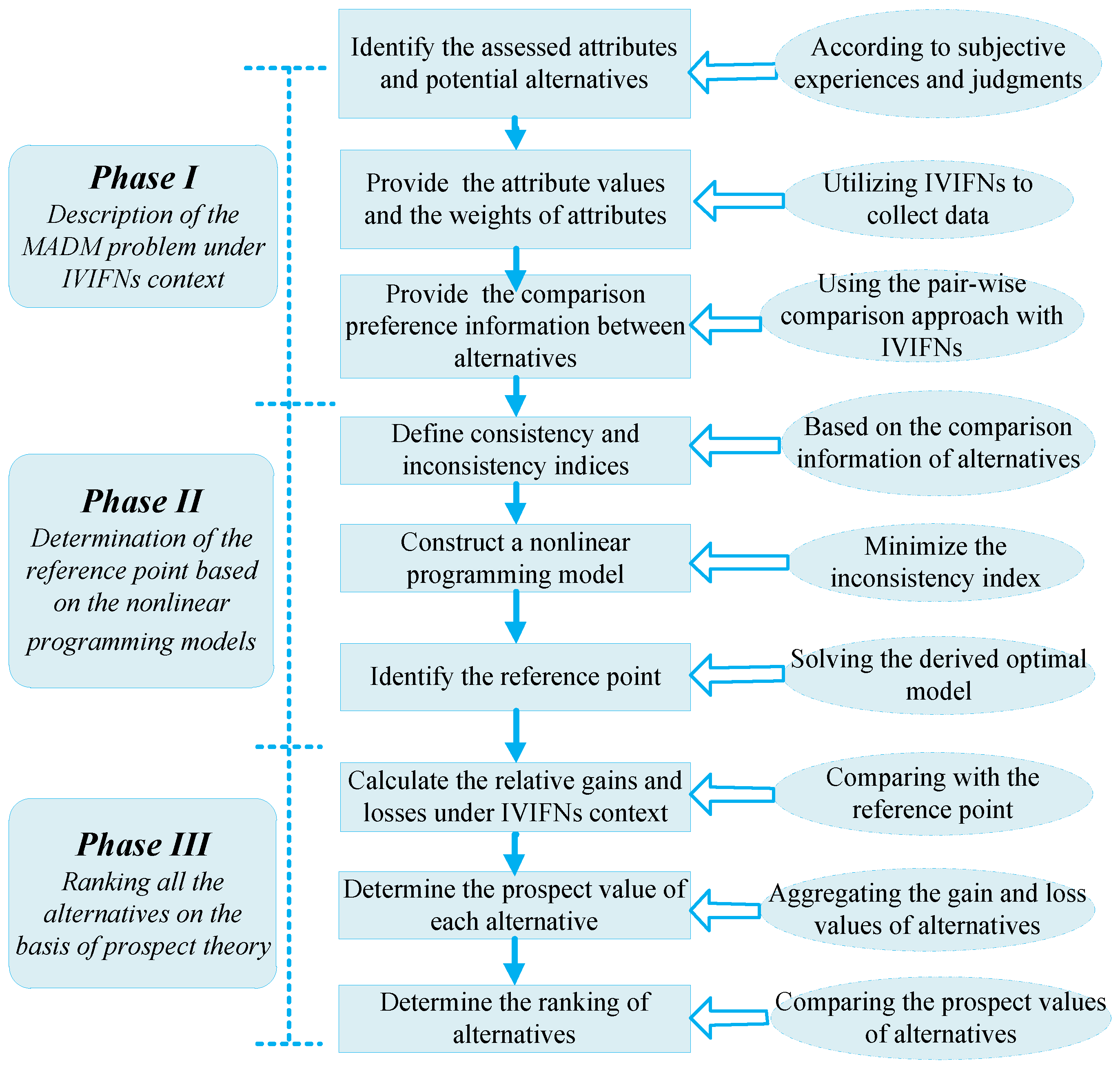
3.3. The Decision Process of the Proposed Approach
4. Case Study
4.1. Description
4.2. Illustration of the Proposed Approach
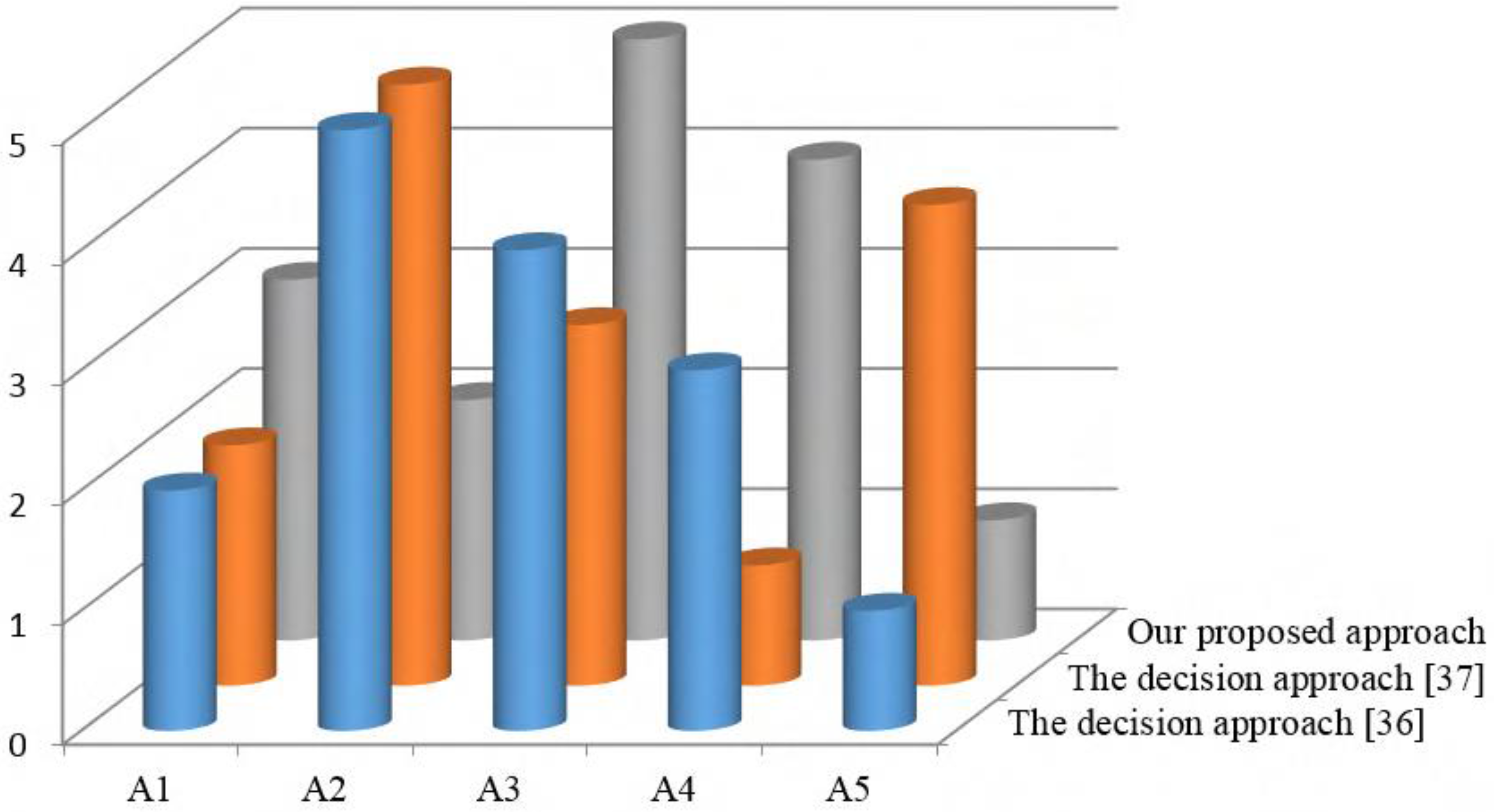
4.3. Discussion and Comparative Analysis
5. Conclusions
Acknowledgments
Author Contributions
Conflicts of Interest
Appendix A
The Proof of Theorem 3.1
References
- Lee, A.H.; Chen, H.H.; Kang, H.-Y. A model to analyze strategic products for photovoltaic silicon thin-film solar cell power industry. Renew. Sustain. Energy Rev. 2011, 15, 1271–1283. [Google Scholar] [CrossRef]
- Srinivasan, V.; Shocker, A.D. Linear programming techniques for multidimensional analysis of preferences. Psychometrika 1973, 38, 337–369. [Google Scholar] [CrossRef]
- Hwang, C.L.; Yoon, K.S. Multiple Attibute Decision Methods and Applications; Springer: Berlin/Heidelberg, Germany, 1981. [Google Scholar]
- Opricovic, S.; Tzeng, G.H. Multicriteria planning of post-earthquake sustainable reconstruction. Comput. Aided Civil Infrastruct. Eng. 2002, 17, 211–220. [Google Scholar] [CrossRef]
- Park, J.H.; Cho, H.J.; Kwun, Y.C. Extension of the VIKOR method for group decision making with interval-valued intuitionistic fuzzy information. Fuzzy Optim. Decis. Mak. 2011, 10, 233–253. [Google Scholar] [CrossRef]
- Roy, B. Classement et choix en présence de points de vue multiples. RAIRO Oper. Res. Rech. Opér. 1968, 2, 57–75. [Google Scholar]
- Hashemi, S.S.; Hajiagha, S.H.R.; Zavadskas, E.K.; Mahdiraji, H.A. Multicriteria group decision making with ELECTRE III method based on interval-valued intuitionistic fuzzy information. Appl. Math. Model. 2016, 40, 1554–1564. [Google Scholar] [CrossRef]
- Govindan, K.; Khodaverdi, R.; Vafadarnikjoo, A. Intuitionistic fuzzy based DEMATEL method for developing green practices and performances in a green supply chain. Expert Syst. Appl. 2015, 42, 7207–7220. [Google Scholar] [CrossRef]
- Zavadskas, E.K.; Antucheviciene, J.; Hajiagha, S.H.R.; Hashemi, S.S. Extension of weighted aggregated sum product assessment with interval-valued intuitionistic fuzzy numbers (WASPAS-IVIF). Appl. Soft Comput. 2014, 24, 1013–1021. [Google Scholar] [CrossRef]
- Xia, H.C.; Li, D.F.; Zhou, J.Y.; Wang, J.M. Fuzzy LINMAP method for multiattribute decision making under fuzzy environments. J. Comput. Syst. Sci. 2006, 72, 741–759. [Google Scholar] [CrossRef]
- Wan, S.P.; Li, D.F. Atanassov's intuitionistic fuzzy programming method for heterogeneous multiattribute group decision making with Atanassov's intuitionistic fuzzy truth degrees. IEEE Trans. Fuzzy Syst. 2014, 22, 300–312. [Google Scholar] [CrossRef]
- Li, D.F. Extension of the LINMAP for multiattribute decision making under Atanassov’s intuitionistic fuzzy environment. Fuzzy Optim. Decis. Mak. 2008, 7, 17–34. [Google Scholar] [CrossRef]
- Zhang, X.; Xu, Z. Interval programming method for hesitant fuzzy multi-attribute group decision making with incomplete preference over alternatives. Comput. Ind. Eng. 2014, 75, 217–229. [Google Scholar] [CrossRef]
- Zhang, X.; Xu, Z.; Xing, X. Hesitant fuzzy programming technique for multidimensional analysis of hesitant fuzzy preferences. OR Spectrum 2016, 38, 789–817. [Google Scholar] [CrossRef]
- Chen, T.Y. An interval-valued intuitionistic fuzzy LINMAP method with inclusion comparison possibilities and hybrid averaging operations for multiple criteria group decision making. Knowl. Based Syst. 2013, 45, 134–146. [Google Scholar] [CrossRef]
- Hajiagha, S.H.R.; Hashemi, S.S.; Zavadskas, E.K.; Akrami, H. Extensions of LINMAP model for multi criteria decision making with grey numbers. Technol. Econ. Dev. Econ. 2012, 18, 636–650. [Google Scholar] [CrossRef]
- Camerer, C. Bounded rationality in individual decision making. Exp. Econ. 1998, 1, 163–183. [Google Scholar] [CrossRef]
- Kahneman, D.; Tversky, A. Prospect theory: An analysis of decision under risk. Econometrica 1979, 47, 263–291. [Google Scholar] [CrossRef]
- Gomes, L.F.A.M.; Lima, M.M.P.P. TODIM: Basics and application to multicriteria ranking of projects with environmental impacts. Found. Comput. Decis. Sci. 1992, 16, 113–127. [Google Scholar]
- Gomes, L.F.A.M.; Rangel, L.A.D.; Maranhão, F.J.C. Multicriteria analysis of natural gas destination in Brazil: An application of the TODIM method. Math. Comput. Model. 2009, 50, 92–100. [Google Scholar] [CrossRef]
- Gomes, L.F.A.M.; Machado, M.A.S.; Rangel, L.A.D. Behavioral multi-criteria decision analysis: The TODIM method with criteria interactions. Ann. Oper. Res. 2013, 211, 531–548. [Google Scholar] [CrossRef]
- Passos, A.C.; Teixeira, M.G.; Garcia, K.C.; Cardoso, A.M.; Gomes, L.F.A.M. Using the TODIM-FSE method as a decision-making support methodology for oil spill response. Comput. Oper. Res. 2014, 42, 40–48. [Google Scholar] [CrossRef]
- Liu, P.D.; Jin, F.; Zhang, X.; Su, Y.; Wang, M.H. Research on the multi-attribute decision-making under risk with interval probability based on prospect theory and the uncertain linguistic variables. Knowl. Based Syst. 2011, 24, 554–561. [Google Scholar] [CrossRef]
- Krohling, R.A.; de Souza, T.T.M. Combining prospect theory and fuzzy numbers to multi-criteria decision making. Expert Syst. Appl. 2012, 39, 11487–11493. [Google Scholar] [CrossRef]
- Krohling, R.A.; Pacheco, A.G.C.; Siviero, A.L.T. IF-TODIM: An intuitionistic fuzzy TODIM to multi-criteria decision making. Knowl. Based Syst. 2013, 53, 142–146. [Google Scholar] [CrossRef]
- Liu, Y.; Fan, Z.-P.; Zhang, Y. Risk decision analysis in emergency response: A method based on cumulative prospect theory. Comput. Oper. Res. 2014, 42, 75–82. [Google Scholar] [CrossRef]
- Fan, Z.-P.; Zhang, X.; Chen, F.-D.; Liu, Y. Multiple attribute decision making considering aspiration-levels: A method based on prospect theory. Comput. Ind. Eng. 2013, 65, 341–350. [Google Scholar] [CrossRef]
- Zhang, X.L.; Xu, Z.S. The TODIM analysis approach based on novel measured functions under hesitant fuzzy environment. Knowl. Based Syst. 2014, 61, 48–58. [Google Scholar] [CrossRef]
- Atanassov, K.; Gargov, G. Interval valued intuitionistic fuzzy sets. Fuzzy Sets Syst. 1989, 31, 343–349. [Google Scholar] [CrossRef]
- Xu, Z.S. Methods for aggregating interval-valued intuitionistic fuzzy information and their application to decision making. Control Decis. 2007, 2, 215–219. [Google Scholar]
- Wang, Z.J.; Li, K.W.; Xu, J.H. A mathematical programming approach to multi-attribute decision making with interval-valued intuitionistic fuzzy assessment information. Expert Syst. Appl. 2011, 38, 12462–12469. [Google Scholar] [CrossRef]
- Wang, Z.; Li, K.W.; Wang, W. An approach to multiattribute decision making with interval-valued intuitionistic fuzzy assessments and incomplete weights. Inform. Sci. 2009, 179, 3026–3040. [Google Scholar] [CrossRef]
- Xu, Z.S.; Chen, J. An overview of distance and similarity measures of intuitionistic fuzzy sets. Int. J. Uncertain. Fuzziness Knowl. Based Syst. 2008, 16, 529–555. [Google Scholar] [CrossRef]
- Ishibuchi, H.; Tanaka, H. Multiobjective programming in optimization of the interval objective function. Eur. J. Oper. Res. 1990, 48, 219–225. [Google Scholar] [CrossRef]
- García-Cascales, M.S.; Lamata, M.T.; Sánchez-Lozano, J.M. Evaluation of photovoltaic cells in a multi-criteria decision making process. Ann. Oper. Res. 2012, 199, 373–391. [Google Scholar] [CrossRef]
- Park, J.H.; Park, I.Y.; Kwun, Y.C.; Tan, X. Extension of the TOPSIS method for decision making problems under interval-valued intuitionistic fuzzy environment. Appl. Math. Model. 2011, 35, 2544–2556. [Google Scholar] [CrossRef]
- Wang, Z.-J.; Li, K.W. An interval-valued intuitionistic fuzzy multiattribute group decision making framework with incomplete preference over alternatives. Expert Syst. Appl. 2012, 39, 13509–13516. [Google Scholar] [CrossRef]
- Zhang, X.; Xu, Z. Extension of TOPSIS to multiple criteria decision making with Pythagorean fuzzy sets. Int. J. Intell. Syst. 2014, 29, 1061–1078. [Google Scholar] [CrossRef]
- Zhang, X. Multicriteria Pythagorean fuzzy decision analysis: a hierarchical QUALIFLEX approach with the closeness index-based ranking methods. Inform. Sci. 2016, 330, 104–124. [Google Scholar] [CrossRef]
- Zhang, X.; Xu, Z.; Wang, H. Heterogeneous multiple criteria group decision making with incomplete weight information: A deviation modeling approach. Inf. Fusion 2015, 25, 49–62. [Google Scholar] [CrossRef]
- Tong, S.C. Interval number and fuzzy number linear programmings. Fuzzy Sets Syst. 1994, 66, 301–306. [Google Scholar]


| Decision Phases | Main Steps |
|---|---|
| Description of the MADM problems under IVIFNs context (Phase I) | Step 1: Identify the evaluation attributes and the feasible alternatives. |
| Step 2: Provide the ratings of alternatives with attributes by using IVIFNs and the weights of attributes. | |
| Step 3: Give the incomplete pairwise comparison preference information between alternatives by using IVIFNs. | |
| Determination of the reference point based on nonlinear programming models (Phase II) | Step 4: Calculate the consistency and inconsistency indices by using Equations (9) and (12), respectively. |
| Step 5: Construct the nonlinear programming model by using the model (MOD-3). | |
| Step 6: Get the reference point vector through solving the model (MOD-3) which is converted into the model (MOD-7). | |
| Ranking all the alternatives based on prospect theory (Phase III) | Step 7: Calculate the prospect values of the alternatives with respect to attributes by using Equation (17). |
| Step 8: Calculate the collective prospect values of alternatives by using Equation (18). | |
| Step 9: Rank these alternatives and the best alternative with the biggest collective prospect value is selected. |
| Alternatives | C1 | C2 | C3 | C4 | |
|---|---|---|---|---|---|
| Attributes | |||||
| A1 | ([0.5, 0.6],[0.2, 0.3]) | ([0.3, 0.4],[0.4, 0.6]) | ([0.4, 0.5],[0.3, 0.5]) | ([0.3, 0.5],[0.4, 0.5]) | |
| A2 | ([0.3, 0.5],[0.4, 0.5]) | ([0.1, 0.3],[0.2, 0.4]) | ([0.7, 0.8],[0.1, 0.2]) | ([0.1, 0.2],[0.7, 0.8]) | |
| A3 | ([0.6, 0.7],[0.2, 0.3]) | ([0.3, 0.4],[0.4, 0.5]) | ([0.5, 0.8],[0.1, 0.2]) | ([0.1, 0.2],[0.5, 0.8]) | |
| A4 | ([0.5, 0.7],[0.1, 0.2]) | ([0.2, 0.4],[0.5, 0.6]) | ([0.4, 0.6],[0.2, 0.3]) | ([0.2, 0.3],[0.4, 0.6]) | |
| A5 | ([0.1, 0.4],[0.3, 0.5]) | ([0.7, 0.8],[0.1, 0.2]) | ([0.5, 0.6],[0.2, 0.3]) | ([0.2, 0.3],[0.5, 0.6]) | |
| Alternatives | C1 | C2 | C3 | C4 | |
|---|---|---|---|---|---|
| Attributes | |||||
| A1 | −1.5199 | −0.5814 | 0.5843 | 0.4805 | |
| A2 | −1.3439 | −0.6732 | 0.5891 | 0.5949 | |
| A3 | −1.6658 | −0.5720 | 0.4591 | 0.4669 | |
| A4 | −1.5678 | −0.5006 | 0.4814 | 0.4283 | |
| A5 | −1.0318 | 0.5130 | 0.5384 | 0.4932 | |
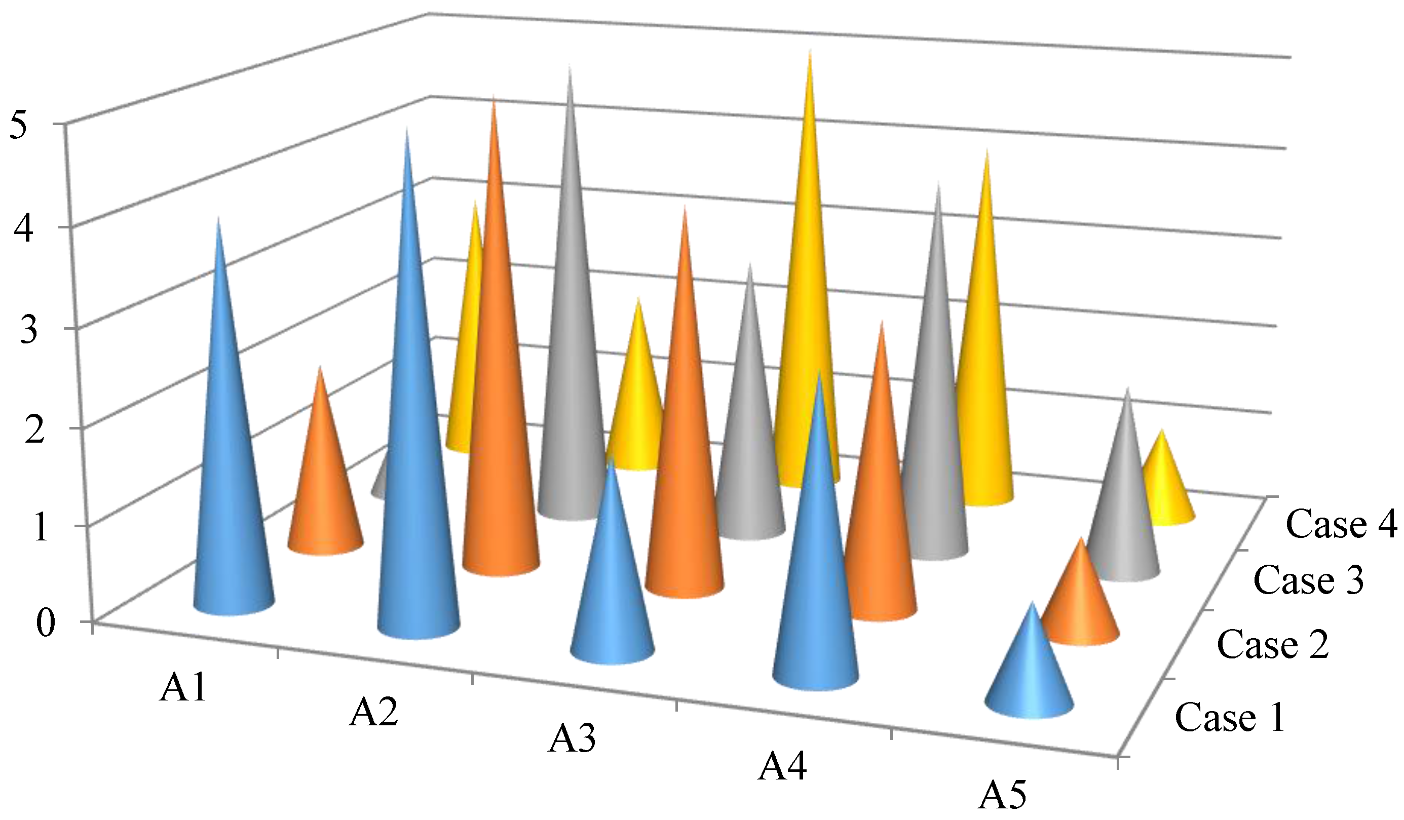
| Different Reference Points | A1 | A2 | A3 | A4 | A5 | The Ranking Orders of Alternatives |
|---|---|---|---|---|---|---|
| Case 1 | −0.2181 | −0.2992 | −0.1032 | −0.1881 | 0.0035 | |
| Case 2 | −0.3178 | −0.3820 | −0.3744 | −0.3497 | 0.1105 | |
| Case 3 | −0.015 | −0.141 | −0.0801 | −0.1253 | 0.0596 | |
| The proposed method (Case 4) | 0.0035 | 0.1105 | 0.5384 | 0.5384 | 0.4932 |
© 2016 by the author; licensee MDPI, Basel, Switzerland. This article is an open access article distributed under the terms and conditions of the Creative Commons Attribution (CC-BY) license (http://creativecommons.org/licenses/by/4.0/).
Share and Cite
Zhang, X. New Interval-Valued Intuitionistic Fuzzy Behavioral MADM Method and Its Application in the Selection of Photovoltaic Cells. Energies 2016, 9, 835. https://doi.org/10.3390/en9100835
Zhang X. New Interval-Valued Intuitionistic Fuzzy Behavioral MADM Method and Its Application in the Selection of Photovoltaic Cells. Energies. 2016; 9(10):835. https://doi.org/10.3390/en9100835
Chicago/Turabian StyleZhang, Xiaolu. 2016. "New Interval-Valued Intuitionistic Fuzzy Behavioral MADM Method and Its Application in the Selection of Photovoltaic Cells" Energies 9, no. 10: 835. https://doi.org/10.3390/en9100835