Article

Operation Modeling of Power Systems Integrated with Large-Scale New Energy Power Sources

1
State Key Laboratory of Alternate Electrical Power System with Renewable Energy Sources, North China Electric Power University, Changping District, Beijing 102206, China
2
School of Electrical and Electronic Engineering, Huazhong University of Science and Technology, Wuhan 430074, Hubei, China
3
State Power Economic Research Institute, Changping District, Beijing 102209, China
*
Author to whom correspondence should be addressed.
Energies 2016, 9(10), 810; https://doi.org/10.3390/en9100810
Submission received: 2 August 2016 / Revised: 20 September 2016 / Accepted: 30 September 2016 / Published: 11 October 2016

Abstract

:
In the most current methods of probabilistic power system production simulation, the output characteristics of new energy power generation (NEPG) has not been comprehensively considered. In this paper, the power output characteristics of wind power generation and photovoltaic power generation are firstly analyzed based on statistical methods according to their historical operating data. Then the characteristic indexes and the filtering principle of the NEPG historical output scenarios are introduced with the confidence level, and the calculation model of NEPG’s credible capacity is proposed. Based on this, taking the minimum production costs or the best energy-saving and emission-reduction effect as the optimization objective, the power system operation model with large-scale integration of new energy power generation (NEPG) is established considering the power balance, the electricity balance and the peak balance. Besides, the constraints of the operating characteristics of different power generation types, the maintenance schedule, the load reservation, the emergency reservation, the water abandonment and the transmitting capacity between different areas are also considered. With the proposed power system operation model, the operation simulations are carried out based on the actual Northwest power grid of China, which resolves the new energy power accommodations considering different system operating conditions. The simulation results well verify the validity of the proposed power system operation model in the accommodation analysis for the power system which is penetrated with large scale NEPG.

1. Introduction

The technique of power system operation simulation is commonly used to simulate the annual and monthly operating states of all the power generation in a system considering the different boundary conditions of the actual power grid, the different operating characteristics of all kinds of generators, and the utilization efficiency of the new energy power generation (NEPG) and the hydroelectric power generation [1,2,3]. In recent years, NEPG (which in this paper mainly refers to wind power generation and photovoltaic (PV) power generation) has experienced fast development in China and reached considerable installed capacity, due to the government policy of limiting carbon emissions and the shortage of primary energy resources. Therefore, the operation model of a modern power system which is integrated with large-scale NEPG needs to be carefully reconsidered using correctly established NPEG power output models. An appropriate operation model of a power system considering large-scale integrated NEPG is of great significance for the study of the power system peak regulation ability investigation and the power generation accommodation assessment.
Current literatures on the stochastic production simulation algorithms of power systems mainly include the piecewise linear approximations method [4,5], the slab method [6], the equivalent power function method [7,8,9] and the half-invariant method [10,11,12]. The fundamental idea of all these algorithms is to convert the chronological load curve to a sequential load curve during which process the time information is lost and the time-variant characteristics of wind power and PV power cannot be reflected effectively. The multi-state machine modelling method [13] and Monte Carlo simulation method [14,15] are always used in modeling NEPG output for probabilistic production simulations. The multi-state generator modelling method can reflect well the randomness of power output and gauge the impacts of forced outages on the system reliability and production costs [16]. For example, the wind speed Weibull distribution is used for the stochastic production modelling of wind power based on the equivalent multi-state modeling method [17]. In [18,19], the β-distribution is used for the solar radiation intensity modeling for PV power output modeling, and the PV power output is modelled by the radiation intensity prediction based on the ARMA model [20]. The Monte Carlo simulation method based on the sample statistics is clear and simple, and can provide a comprehensive view of the influencing factors in power system operation [21]. The work in [22] introduces a mixed integer linear programming framework to establish the production schedule. In [23], the system efficiency, environmental protection, economic cost and resource availability are considered in the optimization objectives.
This paper aims to propose an effective power system operation model which considers the operation characteristics of large-scale NEPG and is adaptive for the peak optimization analysis and new energy power accommodation assessment. The power output characteristics of wind power and PV power generations are first analyzed according to the practical historical operating data. Then the characteristic indexes and the filtering principle of the NEPG historical output scenarios are introduced with the confidence level, and the calculation model of NEPG’s credible capacity is proposed. Based on this, the operation model of power system with large-scale NEPG integrated is established considering the optimization objectives of minimum total costs of the power system and the power balance constraints. A series of comparative operation simulations based on the actual Northwest power grid of China are carried out considering different system operating conditions. With the simulation results, the validity of the proposed power system operation model in NEPG accommodation analysis of the power system with large scale NEPG penetration has been well verified.

2. NEPG Output Characteristics

The output characteristics of wind power generation and PV power generation are largely dependent on the wind source and illumination source, which display strong randomness and volatility. Therefore, the power output prediction of wind power generation and PV power generation requires abundant meteorological information and practical test data, which always have limited accuracy. However, the method based on statistics is proved appropriate to investigate the output characteristics of wind power generation and PV power generation.

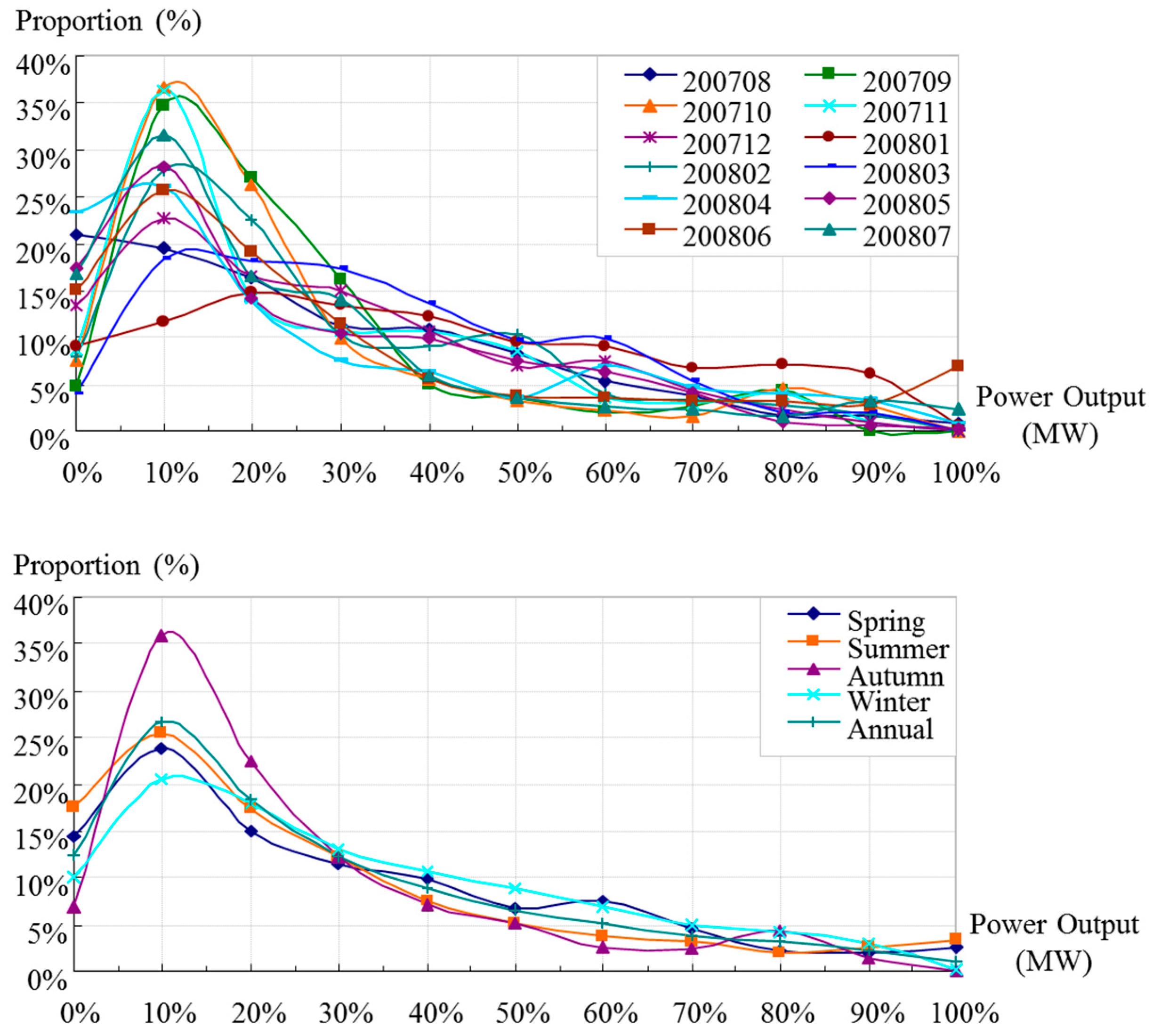
2.1. Wind Power Output Characteristics

According to the practical time-series power output data of the test wind farms of Gansu Province in 2007~2008 [24], the indexes of wind power output characteristics, which are outlined below, are extracted and analyzed statistically on an hourly time scale:
(1) The wind power output shows a positive skewed distribution, and reached the top probability with 10% rated output as shown in Figure 1. When the statistical period extends, the probability distribution curve tends to be smoother (due to space limitations, the following results are indicated with the conclusions only, but no figures).
(2) The cumulative probability of wind power output is a convex quadratic distribution. When the statistical period is extended, the cumulative probability distribution curve tends to be smoother.
(3) The daytime hourly output–guarantee rate of wind power is a concave quadratic distribution, and differs little for different hours.
(4) The hourly output of wind power with different guarantee rates is approximately an even distribution. When the statistical period is extended, the hourly output for different hours tends to be evener.
(5) The wind power output of different hours is highly correlated during a short time period. When the statistical period is extended, the time series correlation distribution tends to be evener.
(6) The wind farm output at the same hour in different days is highly random and volatile during the same season.
(7) The variation probability of wind power output within 10 minutes is approximately a positively skewed distribution. When the wind farm output variation rate is ≤1.5%/min, the probability is more than 99% [25].

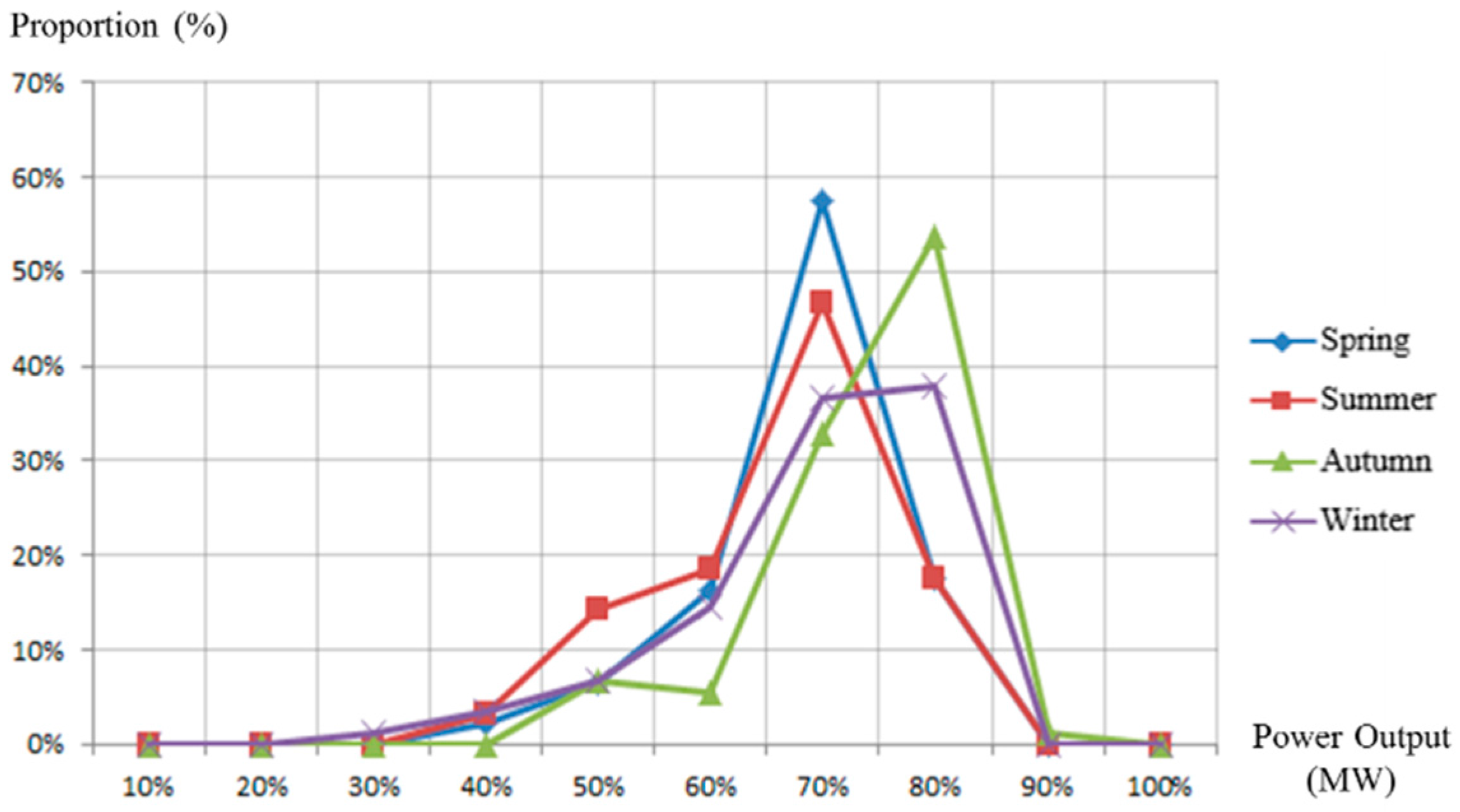
2.2. Photovoltaic Power Output Characteristics

According to the practical time-series power output data of the test PV farms of Qinghai Province in 2007~2008 [24], the indexes of wind power output characteristic are extracted and analyzed statistically using an hourly time scale, as outlined below:
(1) The PV power output is a positively skewed distribution, which reached the top probability with 70% rated output as shown in Figure 2. When the statistical period is extended, the probability distribution curve tends to smoother.
(2) The cumulative probability of PV power output is a convex quadratic distribution of which the noontime hour in X-axis is generally the symmetry axis. When the statistical period is extended, the cumulative probability distribution curve tends to be smoother.
(3) The PV power daytime hourly output–guarantee rate is a concave quadratic distribution, and differs obviously for different hours, being higher at noon and lower in the morning and evening.
(4) The variation probability of PV power output within 5 min is approximately a positive skewed distribution. When the wind farm output variation rate is ≤1%/min, the probability is more than 53.4%.

3. NEPG Output Scenarios Filtering

When considering the integration of large-scale NEPG into a power system, it’s necessary to select the appropriate NEPG output scenarios with a satisfactory confidence level for the power balance analysis, load peaking analysis, and NEPG utilization assessment. To solve this problem, the characteristic indexes of wind power output scenarios and PV power output scenarios are introduced, respectively. The filtering principal of the wind power and photo power output scenarios are proposed consequently.

3.1. Characteristic Indexes of NEPG Output Scenarios

3.1.1. Characteristic Index of Wind Power Output Scenarios

Taking the impact of wind power output on the power system operation simulation into consideration, and considering the daily response characteristics of the load in month m of the area where the wind farm is integrated, the characteristic index Xim of wind power output scenarios is defined as follows:
(1)
Power output at peak-load period in daytime (WP-PO): in the typical day in month m, the power output of wind farm i at the peak-load period in daytime.
(2)
Peaking capacity (WP-PC): in the typical day in month m, the difference of wind farm output between the peak-load period and valley-load period in daytime.
(3)
Average power output (WP-AO): the average value of wind farm’s daily output in the typical day in month m.
The WP-PO is used for the power balance operation simulation, the WP-PC is used for the peaking balance operation simulation, and the WP-AO is used for the electricity balance operation simulation.

3.1.2. Characteristic index of PV Power Output Scenarios

Considering the inconsistency of the distributions between the daily PV power output and daily load response, the characteristic index Xim of PV power output scenarios is defined as follows:
(1)
Maximum power output during daytime (PV-MO): in the typical day in month m, the maximum output of PV station i in daytime.
(2)
Average power output in daytime (PV-AO): in the typical day in month m, the difference of wind farm output between the peak-load period and valley-load period in daytime.
The PV-MO is used for the power balance and peaking balance operation simulations, and the PV-AO is used for the electricity balance operation simulation. We standardize the characteristic indexes of both the wind power output scenarios and PV power output scenarios from the historical data of month m:
I i m = X i m X i m . min X i m . max X i m . min
where Xim.min and Xim.max stand for the minimum and maximum value of all the characteristic indexes in the history, respectively.

3.2. Filtering Principle of NEPG Output Scenarios

The filtering principle of the wind power output scenarios and PV power output scenarios work in the same way. Provided that the characteristic index Xim of NEPG station i’s output scenarios in the typical day have the same distribution probability compared with the historical data, then it is possible to extract the typical scenario day of NEPG output from the historical scenarios days in the corresponding period with a specified confidence level.
Considering the uncertainty and the safety margin of power system operation, the confidence boundary of NEPG output scenarios is introduced here. We specify a confidence level denoted as α (0 ≤ α ≤ 1), and build up a sequence {Pim} of the NEPG station i’s output scenarios from the historical data, then always exists some scenarios {PWim} among {Pim} of which the probability that the value of IWim larger than {Iim} exceeds α [26]. With a given α, the typical scenario day of NEPG output in the level year is preliminarily filtered, located in the scenario sequences {PWim} which meet the above conditions.
Since wind power and PV power are renewable energy sources so larger characteristic indexes are more favorable for the power system dispatching operation, the confidence boundary of NEPG output scenario is defined as follows: with a identified confidence level α, if there exists some scenarios {PWim} among {Pim} of which the probability that the value of IWim larger than {Iim} exceeds α, the scenario which has the largest value of IWim among {PWim} is defined as the confidence boundary of NEPG output scenario and the corresponding characteristic index of the can be described by [27]:
I W i m | α = max [ I i m : p ( I W i m > I i m ) α ]     α [ 0 , 1 ]
Since [p(IWim > Iim) ≥ α] = [p(IWimIim) < 1 − α], the characteristic index of the confidence boundary of NEPG output scenario can also be described by:
I W i m | α = max [ I i m : p ( I W i m I i m ) < 1 α ]
In addition, if known the cumulative probability distribution function F(IWim) or the probability density function f(IWim) of the characteristic index, the probability that IwimIim can be expressed by [28]:
p ( I W i m > I i m ) = I i m 1 f ( I W i m ) d I i m = 1 F ( I W i m )
With the above definition of the confidence boundary scenario, the filtering process of the typical scenario day of NEPG output in month m in the level year is as follows:
(1) Sequence the historical scenarios
Build up the sequence {Pim} of the NEPG station i’s output scenarios in month m from the historical data, sequence them according to the order of the value of Iim, as follows:
I i m ( 1 ) I i m ( 2 ) I i m ( k ) I i m ( n )
where Iim(k) is the characteristic index of the kth scenario Pim(k); n is the total number of historical scenarios.
(2) Construct the cumulative probability distribution function of the characteristic indexes
Based on (5), the cumulative probability distribution function of the characteristic indexes of NEPG station i in month m in history can be calculated by [26]:
F ( I W i m ) = { 0 , I i m < I i m ( 1 ) k n , I i m ( k ) I i m < I i m ( k + 1 ) , k = 1 , 2 , ... , n 1 1 , I i m I i m ( n )
(3) Filter the typical scenario day
According to Equations (2)–(4), the characteristic index of the NEPG output confidence boundary IWim|α can be obtained by the cumulative probability distribution function from the historical characteristic indexes with a given confidence level. Since the cumulative probability distribution function is a step function but not a continuous function, the characteristic index of the scenario which is closest to the confidence boundary scenario is set as the boundary index IWim|α, calculated by:
[ F ( I i m ( j ) ) ( 1 α ) ] [ F ( I i m ( j + 1 ) ) ( 1 α ) ] 0 ( 1 α ) F ( I i m ( j ) ) F ( I i m ( j + 1 ) ) ( 1 α )
[ F ( I i m ( j 1 ) ) ( 1 α ) ] [ F ( I i m ( j 1 ) ) ( 1 α ) ] 0 F ( I i m ( j ) ) ( 1 α ) ( 1 α ) F ( I i m ( j 1 ) )
where Iim(j) is the characteristic index of wind farm output confidence boundary under the confidence level α. With the determined IWim|α, the corresponding wind power output scenario PWim|α is also assured, set as the wind power output typical day in month m in the lever year.

3.3. Credible Capacity Resolution of NEPG

In the production operation simulation of a power system, a credible NEPG capacity needs to be calculated to make an accurate assessment of the NEPG utilization. The utilized capacity of NEPG station i in area s at hour t in the typical day in month m in the level year is described by:
P U T s m t = P A V s m t P W s m t
where PAVsmt and PWsmt are the total amount of the available capacity and the wasted capacity of NEPG station i in area s at hour t in the typical day in month m in the level year, respectively.
The total amount of the generated electricity and the available electricity of NEPG station i in area s at hour t in the typical day in month m in the level year are described by:
{ E s m = i s t = 1 24 P U T i m t E A V s m = i s t = 1 24 P A V i m t
The total amount of the generated electricity and the available electricity of NEPG station i in area s in month m in the level year are described by:
{ E M s m = i s w = 1 7 t = 1 24 P U T i m w t / K m E M A V s m = i s w = 1 7 t = 1 24 P A V i m w t / K m
where PUTWimwt and PAVWimwt are the utilized capacity and available capacity of NEPG station i at hour t in the typical day in typical week w in month m in the level year, respectively. Km is the conversion factor between the weekly generating capacity and the monthly generating capacity of NEPG, described as Km = day number in month m/7.
The daily utilization hour of wind power in a typical day in month m in the level year:
T s m = E s m / i s C i
where Ci is the rated capacity of NEPG station i.

4. Power System Operation Modeling Considering Large-Scale NEPG Integration

4.1. Objective Function

In this work, the main optimization objective of the power system operation simulation considering large-scale integrated NEPG is set as the lowest power generation cost or the best energy saving effect. The sub-series optimization objectives also include the optimization of areas power exchange, the optimization of thermal power plants’ boot capacity, and the optimization of the unit commitment scheme of different generation types. In the optimization process, the technical and economic characteristics of different power generation types are not identical, and their contributions to the power system operation optimization also differs. Besides this, several other technical and economic indicators are also considered, such as: (1) the power plant’s maintenance plan; (2) the system load reserve and emergency reserve; (3) the electricity consumption and peak load balance in each area; (4) the annual electricity production, utilization hours, fuel demand and variable operating costs of different generations; (5) the wasted electricity of hydropower stations; and (6) the exchanged power flow between different areas. The objective function is expressed by:
min F ( P ) = min E W Q min { E H Q |   max ( P ¯ H m + R H m ) , m = 1 , 2 , ... , 12 } max { P ¯ P m ( T E , E Q ) + R P m ( T E , E Q ) , m = 1 , 2 , ... , 12 } max { P A m ( T E ) + R A m ( T E ) , m = 1 , 2 , ... , 12 } max { min ( Δ P s m ( n M m ) , m = 1 , 2 , ... , 12 ) } min { F ( P T )   |   max ( min ( Δ P s m , m = 1 , 2 , ... , 12 ) ) min ( Δ E s ) }
where: F(P) represents the total generation cost of the power system; EWQ and EHQ are the wasted electricity of NEPG and hydropower generation, respectively; P ¯ H m and P ¯ P m are the maximum power output of hydropower plants and pumped storage plants in month m in the level year, respectively; PAm is the power output of nuclear generation in month m in the level year; RHm, RPm and RAm are the arranged reserve capacity of hydropower plants, pumped storage plants and nuclear plants in month m, respectively; TE is the expected annual utilization hours; ΔPsm is the electricity surplus in area s in month m in the level year; nMm is the number of maintenance generators in month m in the level year; F(PT) is thermal power generations(or the primary energy consumption, the pollution emissions and the thermal power purchase cost), respectively; ΔEs is the electricity shortage in area s in the level year.

4.2. Restraint Conditions

The power/electricity balance restraints and the generation operating restraints are the two main aspect mainly considered in power system operation simulation with the integration of large-scale NEPG.

4.2.1. Power/Electricity Balance Restraint

(1) Capacity balance restraints:
i s P i m t + l s P L l m t = L s m t
s 0 L s m t = L 0 m t
where Lsmt is the power load of area s at moment t in month m in the level year. Pimt is power output of the hydropower plant i at moment t in month m in the level year. PLlmt is the receiving power of area s through the transmission lines from other areas at moment t in month m in the level year.
(2) Restraint of load reserve and emergency reserve:
{ i s R R i m + l s R L R l m = R R s m R R N s m i s R S i m + l s R L S l m = R S s m
{ s 0 R R s m = R R 0 m s 0 R S s m = R S 0 m
where RRsm and RSsm are the spinning reserve capacity and the cold reserve capacity of area s in month m in the level year, respectively. RRNsm is the lower limit of spinning reserve capacity of area s in month m in the level year. RRim and RSim are the spinning reserve capacity and the cold reserve capacity generated by generator i in month m in the level year, respectively. RLRlm and RLSlm are the receiving spinning reserve capacity and cold reserve capacity of area s through the transmission lines from other areas in month m in the level year.
(3) Peak load balance restraint
i s Δ P i m + l s Δ P L l m Δ L s m + R R s m
where ΔPim and ΔPLlm are the peaking capacity of the power plant i and transmission line l in the typical day in month m in the level year, respectively. ΔLsm is the load peak-valley difference of area s in month m in the level year.
(4) Restraint of maximum transmission line capability:
C L l m P L l m t + R L R l m + R L S l m C L + l m
where CL+lm and CL-lm are the maximum receiving capacity and maximum exporting capacity in transmission line l in month m in the level year.
(5) Electricity balance restraint:
i s E i m + l s E L l m = E s m s 0 E s m = E 0 m
where Esm is the forecasting load of area s in month m in the level year. Eim is the generation capacity of power plant i in month m in the level year. ELlm is the receiving electricity of area s through transmission line l in month m in the level year.
(6) Security boot constraint:
i s n T i m C i + i s n A i m C i C s min
where nTim and nAim are the boot numbers of thermal plants and nuclear plants in the level year, respectively. Ci is the capacity of power plant i. Csmin is the security boot capacity of area s.
(7) Restraint of lower limit of thermal plant’s spinning reserve capacity:
i s R T R i m R T s min R R s m
where RTRim is the spinning reserve capacity of thermal plant i in month m in the level year, and RTsmin is the proportion of thermal plant i’s spinning reserve capacity in the total amount of area s.
(8) Restraint of reserve capacity upper limit of hydropower plants and pumped storage power plants:
i s R H i m + i s R P i m R H s max ( R R s m + R S s m )
where RHim and RPim are the reserve capacity of hydropower plant and pumped storage plant i in month m in the level year, respectively, and RHsmax is the corresponding proportion of plant i’s reserve capacity in the total amount of area s.
(9) Maintenance ability restraint of thermal plants
R M s min C T s i s n T M i m C i R M s max C T s
where RMsmax and RMsmin are the upper limit and lower limit of thermal plant’s maintenance ability, respectively. CTs is the total installed capacity of the thermal plants in area s. nTMim is the number of the planned maintained generator in month m in the level year.
(10) Restraint of the emission of CO2, SO2, NOx and soot
{ i s C O E i C O E s max i s S O E i S O E s max i s N O E i N O E s max i s D S E i D S E s max
where COEi, SOEi, NOEi and DSEi are the CO2, SO2, NOx and soot emissions of power plant i in the level year, respectively. COEsmax, SOEsmax, NOEsmax and DSEsmax are the upper limit of CO2, SO2, NOx and soot emissions of area s in the level year.

4.2.2. Generation Operating Restraints

(1) Output restraint:
P _ i m P i m t P ¯ i m
where P ¯ m and Pim are the upper limit and lower limit of the power plant i’s output in month m in the level year, respectively.
(2) Reserve capacity restraint:
0 R i m R i max
where Ri is the power plant i’s reserve capacity in month m in the level year, and Rimax is the upper limit of Ri.
(3) Energy consumption restraint (represented by utilization hours):
T _ i T i m T ¯ i
where Tim is the power plant i’s annual utilization hour in the level year, and T ¯ i and T _ i are the upper limit and lower limit of Tim.
(4) Maintenance restraint:
n M i m n ¯ M i
where n M i m is the actual maintained number of power plant and n ¯ M i is the upper limit.
(5) Electricity balance restraint of hydropower plants:
t = 1 24 × D m ( P H i m t + P Q i m t ) = 24 D m P H A V i m
where PHAVim is the average output of hydropower plant i in month m, PHimt is the output at hour t, and PQimt is the abandoned electricity in load peaking. Dm is the number of the days in month m.
(6) Daily electricity balance restraint of pumped storage plants:
t = 1 24 P P i m t = η i t = 1 24 L P i m t
E P V m t = t = 1 24 L P i m t E P V i
where EPVi and ηi are the max pumping capacity and the pumping-power conversion efficiency of the pumped storage plant i. E P V m , P P i m t and L P i m t are the pumping power in the typical day, power output at hour t, and pumping load of the pumped storage plant i in month m in the level year, respectively.
(7) Operating quantity restraint of thermal plants:
n _ i m n T i m n ¯ i m
where n ¯ i m and n _ i m are the upper limit and lower limit of the operating quantity of thermal plant i in month m in the level year, respectively.
(8) Start-off time restraint of thermal plants in load peaking:
t R i m t _ R i     t S i m t _ S i
where tRim and tSim are the continuous boot hour and the continuous shutdown hour of the thermal plant i when during peaking period in the typical day in month m in the level year, respectively. tRi and tSi are the lower limit of the continuous boot hour and the continuous shutdown hour, respectively.

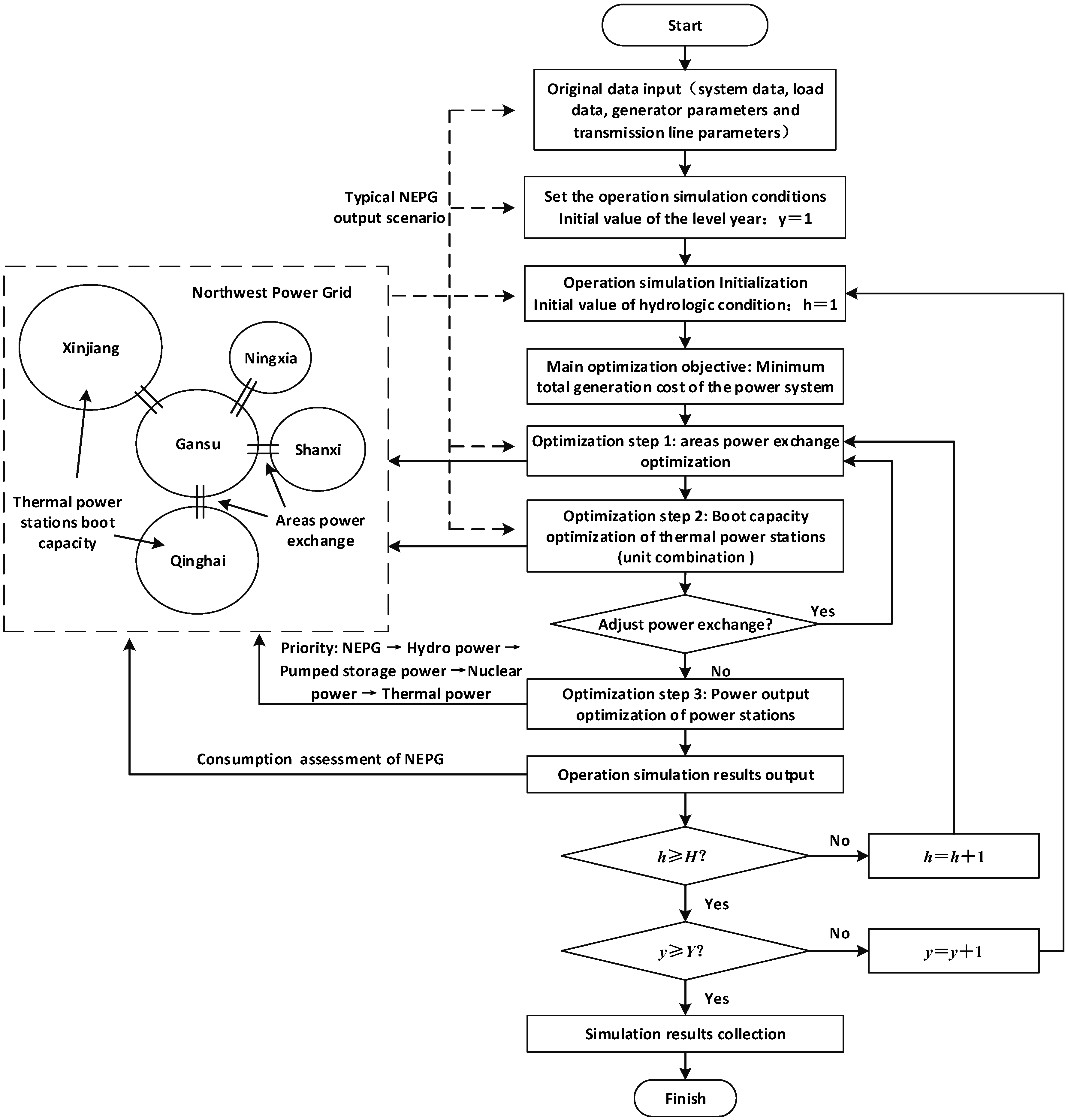
4.3. Power System Operation Simulation Process

In this work, taking the technical and economic characteristics of different power generation types, and the specific power output scenarios of wind power generation and PV power generation into consideration, a power system operation simulation is conducted:
(1) Firstly, considering the limits of transmission capacity between different areas, the technical and economic characteristics of different power generations are evaluated. Applied with the sub- optimization processes on unit generation prioritizing, load distributing, load peaking and unit maintenance/reservation arrangement, the best area power exchange results are calculated to achieve the optimal technical and economic effect of all generation types.
(2) Then, according to the power balance of each area, the boot capacity of thermal power plants and unit combinations are optimized. When the peaking capacity of an area is lacking, the output of NEPG in other areas which transmit power into this area are previously reduced, and then we get the NEPG in the local area.
(3) Finally, with the optimized shutdown schedule of all the power plants, the detailed operating point and generation capacity of each power plant are calculated, according to the priority sequence of “New energy power → Hydro power → Pumped storage power → Nuclear power → Thermal power”.
The operation simulation process of a multi-provinces interconnected power system considering the characteristics of large-scale integrated NEPG is shown in Figure 3.

5. Simulation Analysis

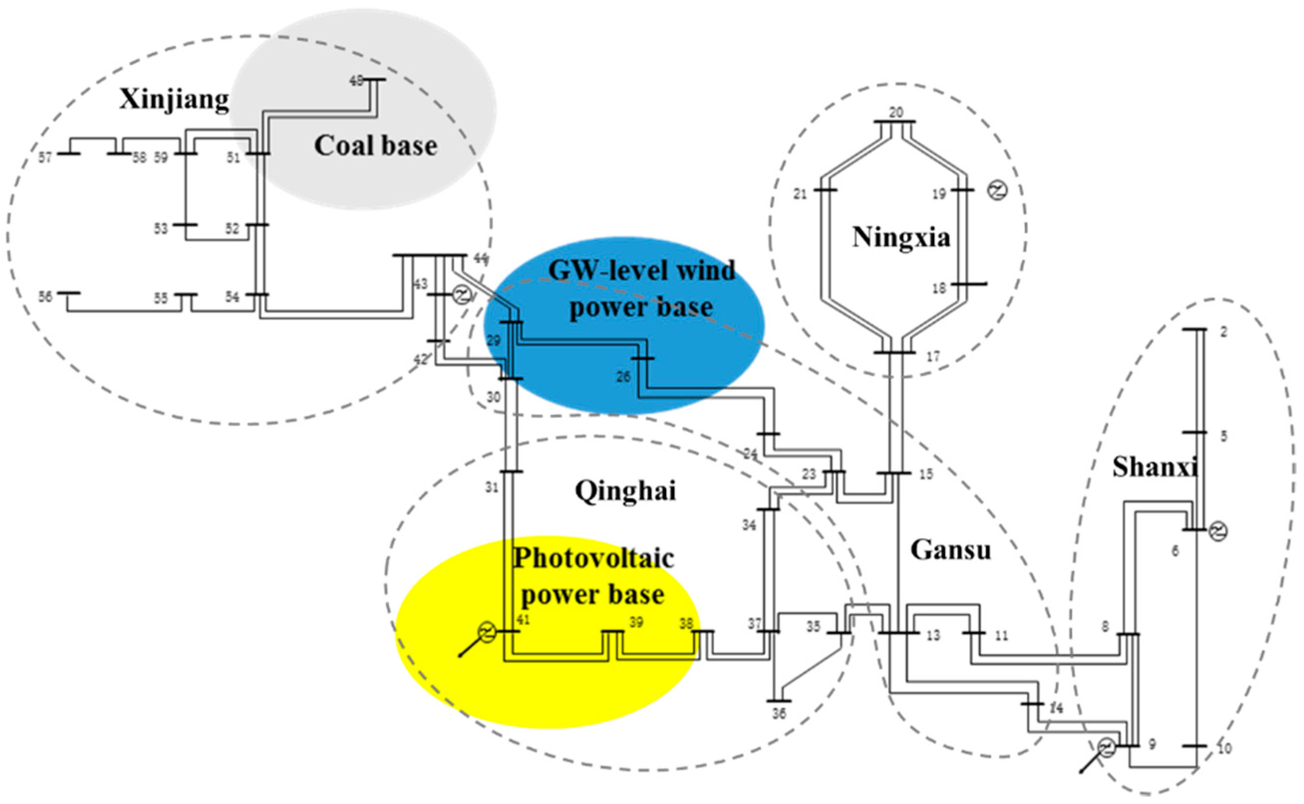
5.1. Simulation Models

The power system operation simulation is carried out on the power system operation simulation software SPER-ProS, developed by the State Grid Corporation of China. The simulation model is established based on the Northwest power grid of China, which contains diverse energy resources and is integrated with large-scale thermal power, hydropower, wind power and PV power generations. Based on the power system operation model proposed above, the accommodation capability of NEPG in the five northwestern provinces are investigated through the power system operation simulation, in which the practical data of power loads, power exchanges between provinces, installed capacity of power plants, and power output characteristics of NEPG are utilized.
The 750 kV-level power grid structure of the Northwest power grid of China in 2014 is shown in Figure 4. It contains 41,750 kV transformer substations and five high-voltage direct current (HVDC) converter stations. As shown in Figure 4, the grey area represents the planning coal base in Zhundong, Xinjiang Province, the blue area represents the planning GW-level wind power base in Jiuquan, Gansu Province, and the yellow area represents the planning PV power plants centrally integrated in Qinghai Province.

5.2. Boundary Conditions

Taking the year 2020 as the level year, the total power load of the Northwest power grid is expected to reach 147,010 MW, the installed hydropower capacity is 39,363 MW, the installed thermal power capacity is 222,642 MW, the installed wind power capacity is 75,480 MW, and the installed PV power capacity is 35,000 MW, as shown in Table 1.
Considering the influence of the Hexi Corridor on the NEPG accommodation of the Northwest power grid, the Gansu power grid is modelled divided into three districts: the west, the central and the east, among which the west part is mainly referred to as the new energy centralized-integrated area which includes Jiuquan and Dunhuang, the central part is also referred to as the new energy centralized-integrated area which includes Jinchang and Wuwei, and the east part consists of the load center which includes East Lanzhou and Baiyin, and the coal base which includes Pingliang and Qingyang. For the same reason, the Qinghai power grid is modelled as divided into two districts: the west and the east, among which the west part mainly refers to the large-scale PV integrated area which includes Haixi and Ge’ermu, and the east part consists of the load center which includes Xining, Riyueshan and Tala, the hydropower integrated area of the upreaches of the Huanghe River, and the PV power integrated area of Hainan.
The power flows of the key transmission sections in province or between provinces are calculated according to the transmission capacity shown as below:
  • The first and second transmission sections between Xinjiang and the Northwest power grid: the maximum forward transmission capacity from Xinjiang to the Northwest power grid is up to 4000 MW and the minimum forward transmission power flow is 800 MW.
  • The transmission section from Xinjiang to Qinghai: the maximum forward and backward transmission capacity is up to 2000 MW and the minimum transmission power flow is 400 MW.
  • The transmission sections between Shanxi and Gansu: the maximum forward and backward transmission capacity are both 6000 MW.
  • The transmission sections between Gansu and Ningxia: the maximum forward and backward transmission capacity are both 6000 MW.
  • The transmission sections between Gansu and Hexi Corridor: the maximum transmission capacity of the 750 kV transmission line from Jiuquan to Hexi is 3000 MW.
In the power system operation simulation, the load peaking by hydropower is considered first, and the minimum output of the thermoelectric plants is 0.8 p.u. with an annual utilization of more than 4500 h.

5.3. NEPG Accommodation Ability Analysis

Based on the power system operation model proposed in this paper, the power output characteristic of NEPG has been taken into full consideration in the optimization process of our power system operation simulation. The NEPG’s accommodation capacity in each province and the transmitted capacity between provinces can be both obtained clearly from the operation simulation results, which is really important for the modern power system operation simulation study with large-scale NEPG integration.
With the boundary conditions described above in the last section, a power system operation simulation of the Northwest power grid of China was conducted and the NEPG accommodation in the five provinces is clearly resolved, as shown in Table 2 and Table 3. The accommodated electricity of NEPG in the global Northwest power grid reaches 1558.5 billion kWh and the wasted electricity is about 458 billion kWh, with the wasted electricity proportion being 22.7%. If the installed capacity of NEPG in the provinces where new energy power is heavily wasted is cut down the wasted electricity proportion of the global Northwest power grid declines to 5%, then the wind power accommodation capacity of the Northwest power grid is 40,910 MW and the PV power reaches 28,760 MW. The rest of the NEPG capacity transmitted to interconnected provinces is 40,810 MW, of which the wind power represents 34,570 MW and the PV power is 6240 MW.
In the situation that if 26,750 MW NEPG is transmitted from the Northwest power grid to other district power grids through the DC transmission lines, including the Hami-Zhengzhou ±800 kV DC transmission line, the Jiuquan-Hunan ±800 kV DC transmission line, the Zhundong-Huainan ±1100 kV DC transmission line, there will be 14,060 MW NEPG left that cannot being accommodated.

5.4. Sensitivity Analysis

With the sensitivity analysis of the thermoelectric plants’ output, the system peak capacity and the transmission lines’ capacity, the NEPG accommodation conditions of the Northwest power gird are further investigated in this section.

5.4.1. Sensitivity Analysis of the Thermoelectric Plants’ Output

In an actual power system, during the early period and the final period of the heating season, the minimum technical output of the thermoelectric plants is generally more than 0.55 p.u. and during the middle period of the heating season, the minimum technical output of the thermoelectric plants is generally more than 0.75 p.u. According to practical surveys that the minimum technical output of the thermoelectric plants can even be adjusted to 0.5 p.u. during the early period and the final period of the heating season, and 0.6 p.u. during the middle period of the heating season. Therefore, compared to the present operation status, there is generally 0.1 to 0.15 p.u. space in the thermoelectric plant’s capacity to peak load. We sdjust the thermoelectric plants’ output according to this margin, and conduct the power system operation simulation again. The power system operation simulation results gives the new accommodation conditions of NEPG showing that the wind power and PV power in the Northwest power grid can be well accommodated.

5.4.2. Sensitivity Analysis of System Peaking Capacity

Based on the boundary conditions described in Section 4.2, in this comparative case, the power system operation simulation is conducted with the minimum power output level of thermal power plant adjusted to 0.7 p.u. from 0.5 p.u., while the minimum technical output of the thermoelectric plants remains the same. The power system operation simulation gives the new NEPG accommodation conditions, and from the simulation results presented in Table 4 and Table 5, the wind power accommodation capacity of the global Northwest power grid declines to 26,160 MW and the PV power accommodation capacity declines to 17,890 MW. It’s suggested that the NEPG accommodation abilities in the five provinces have all been depressed due to the decline of system peaking capacity which is caused by higher minimum technical output of the thermoelectric plants.

5.4.3. Sensitivity Analysis of Transmission Lines’ Capacity

Still based on the above boundary conditions, but in this sensitivity study case the capacity of the transmission lines from Gansu province to other areas is cut down by 2000 MW. The power system operation simulation results are also presented in Table 4 and Table 5. Since the transmission lines from Gansu Province to other areas are the main channel which transmits the electricity generated in Xinjiang and Gansu to the load center in the Northwest power grid, the cutting down in these transmission lines’ capacity directly results in the delineation of the NEPG accommodation in Xinjiang and Gansu provinces. However, the NEPG accommodation in the other three provinces has not been affected.

6. Conclusions

This paper aimed to propose an effective power system operation model which considers the operation characteristics of large-scale NEPG and is adaptive for the peak optimization analysis and new energy power accommodation assessment. The power output characteristics of wind power and PV power generations are firstly analyzed according to the practical operating data. Then the characteristic indexes and the filtering principle of the NEPG historical output scenarios are introduced with the confidence level, and s calculation model of NEPG’s credible capacity is proposed. Based on this, the operation model of power systems with large-scale NEPG integrated is established considering the optimization objectives of minimum total costs of the power system and the power balance constraints. The operation simulation results based on the actual Northwest power grid of China under different system operating conditions shows that the new energy power accommodation can be resolved effectively based on the proposed power system operation model.
Though three kinds of scenarios of wind power output has been taken into consideration in this paper, the objective function of power system operation simulation and the wind power output scenarios are much more complex in actual power systems, which may result in different power system operation models and this needs to be further analyzed in future.

Acknowledgments

This research work was supported by the National High Technology Research and Development Program of China: “Planning Research and Operation Basic Theory of Power Systems with Integration of High Penetration of Renewable Energies”. The authors are grateful for this support.

Author Contributions

Hui Li and Gengyin Li conceived and designed the experiments; Hui Li performed the experiments; Hui Li, Yaowu Wu and Zhidong Wang analyzed the data; Jiaming Wang contributed analysis tools; Hui Li wrote the paper.

Conflicts of Interest

The authors declare no conflict of interest.

References

  1. Lou, S.H.; Lu, S.Y.; Wu, Y.W.; Yin, X.G. An Overview on Low-Carbon Power System Planning and Operation Optimization. Power Syst. Technol. 2013, 6, 1483–1490. [Google Scholar]
  2. Ma, J.; Shi, J.L.; Li, W.Q.; Wang, Z.P. A day-ahead dispatching strategy for power pool composed of wind farms, photovoltaic generations, pumped-storage power stations, gas turbine power plants and energy storage systems based on multi frequency scale analysis. Power Syst. Technol. 2013, 6, 1491–1498. [Google Scholar]
  3. Wu, H.L.; Du, E.; Men, K.; Yang, L.; Su, L.; Lu, S.Y.; Luo, X. A Low-Carbon Oriented Energy-Saving and Economic Operation Evaluation System. Power Syst. Technol. 2015, 5, 1179–1185. [Google Scholar]
  4. Baleriaux, E.J.; Guertechin, L.E. Simulation de I'exploitation d'un Parc de Machines Thermiques de Production d'Electricite Couple a des Stations de Pompage. Revue E 1967, 5, 3–24. [Google Scholar]
  5. Booth, R.R. Power system simulation model based on probability analysis. IEEE Trans. Power Syst. 1972, 91, 62–69. [Google Scholar] [CrossRef]
  6. Schenk, K.F.; Misra, R.B.; Vassos, S. A new method for the evaluating of expected energy generation and loss of probability. IEEE Trans. Power Syst. 1984, 103, 294–303. [Google Scholar] [CrossRef]
  7. Wang, X. Equivalent energy function approach to power system probabilistic modeling. IEEE Trans. Power Syst. 1988, 3, 823–829. [Google Scholar] [CrossRef]
  8. Wang, X. EEF approach to power system probabilistic modeling. J. Xi’an Jiao Tong Univ. 1984, 18, 13–26. [Google Scholar]
  9. Li, L.; Wang, X.; Wang, X. Probabilistic modeling for inter connected power systems based on the equivalent energy function approach. Proc. CSEE 1996, 16, 180–184. [Google Scholar]
  10. Rau, N.S.; Toy, P.; Schenk, K.F. Expected energy production costs by the method moments. IEEE Trans. Power Apparatus Syst. 1980, 99, 1908–1917. [Google Scholar] [CrossRef]
  11. Stremel, J.P.; Jenkins, R.T.; Babb, R.A. Production costing using the cumulant method of representing the equivalent load curve. IEEE Trans. Power Apparatus Syst. 1980, 99, 1947–1956. [Google Scholar] [CrossRef]
  12. Chen, G.; Xiang, N.; Chen, X. A new method for probabilistic production simulation based on load decomposition. Proc. CSEE 1992, 12, 47–52. [Google Scholar]
  13. Liao, Y. Research on power system probabilistic production simulation including wind farms. Master’s Thesis, North China Electric Power University, Beijing, China, 2012. [Google Scholar]
  14. Wang, X.; Dai, H.; Thomas, R.J. Reliability modeling of large wind farms and associated electric utility interface systems. IEEE Trans. Power Apparatus Syst. 1984, 103, 569–575. [Google Scholar] [CrossRef]
  15. Zhang, J.T.; Cheng, H.Z.; Hu, Z.C.; Ma, Z.L.; Zhang, J.P.; Yao, L.Z. Power system probabilistic production simulation including wind farms. Proc. CSEE 2009, 29, 34–39. [Google Scholar]
  16. Billinton, R.; Yi, G.; Karki, R. Application of a joint deterministic-probabilistic criterion to wind integrated bulk power system planning. IEEE Trans. Power Syst. 2010, 25, 1384–1392. [Google Scholar] [CrossRef]
  17. Zou, X. Research of probabilistic production simulation of power system with wind power and efficiency evaluation of wind farm. Master’s Thesis, Xi’an Jiaotong University, Xi’an, China, 2008. [Google Scholar]
  18. Li, Y.; Zio, E. Uncertainty analysis of the adequacy assessment model of a distributed generation system. Renew. Energy 2012, 41, 235–244. [Google Scholar] [CrossRef] [Green Version]
  19. Atwa, Y.M.; ElSaadany, E.F.; Salama, M.M.A. Optimal renewable resource mix for distribution system energy loss minimization. IEEE Trans. Power Syst. 2010, 25, 360–370. [Google Scholar] [CrossRef]
  20. Guo, X.Y.; Xie, K.; Hu, B. A time-interval based probabilistic production simulation of power system with grid-connected photovoltaic generation. Power Syst. Technol. 2013, 37, 1500–1505. [Google Scholar]
  21. Dobakhshari, A.S.; Fotuhi-Firuzabad, M. A reliability model of large wind farms for power system adequacy studies. IEEE Trans. Energy Convers. 2009, 24, 792–801. [Google Scholar] [CrossRef]
  22. Ben-Awuah, E.; Elkington, T.; Askari-Nasab, H.; Blanchfield, F. Simultaneous production scheduling and waste management optimization for an oil sands Application. J. Environ. Inform. 2015, 26, 80–90. [Google Scholar]
  23. Tan, Q.; Huang, G.; Cai, Y. A fuzzy evacuation management model oriented toward the mitigation of emissions. J. Environ. Inform. 2015, 25, 117–125. [Google Scholar] [CrossRef]
  24. Li, H.; Wang, Z.; Guo, F. Research on the Theory and Method of Large Power Network Planning with Large-Scale Centralized Integration of Multi Form Power Generations; State Power Economic Research Institute: Beijing, China, 2013. [Google Scholar]
  25. Li, H.; Wang, Z. Transmission Planning and Designing for the Seven 10 Million kW Level Wind Power Bases; State Power Economic Research Institute: Beijing, China, 2008. [Google Scholar]
  26. Degroot, M.H.; Schervish, M.J. Probability and Statistics; Addison-Wesley: Boston, MA, USA, 2002. [Google Scholar]
  27. Siegmund, D. Sequential Analysis: Tests and Confidence Intervals; Springer Science & Business Media: New York, NY, USA, 2013. [Google Scholar]
  28. Papoulis, A.; Pillai, S.U. Probability, Random Variables, and Stochastic Processes; Tata McGraw-Hill Education: Boston, MA, USA, 2002. [Google Scholar]
Figure 1. Probability distribution curves of wind power output in 2007~2008 of Gansu Province wind farms.
Energies 09 00810 g001
Figure 2. Probability distribution curve of PV power output in 2008 of Qinghai Province PV stations.
Energies 09 00810 g002
Figure 3. The operation flow diagram of a power system integrated with large-scale new energy power.
Energies 09 00810 g003
Figure 4. 750 kV power grid diagram of the Northwest power grid in 2014.
Energies 09 00810 g004
Table 1. The planning power generation capacity of the Northwest power grid.
Generation TypeInstalled Capacity (MW)
Hydropower station39,363
Thermal power station222,642
Wind power station75,480
Photovoltaic power station35,000
Table 2. Wind power accommodation in the Northwest power gird.
Power GridInstalled Capacity (MW)Local Accommodated Power (MW)Outside Transmitted Power (MW)
Northwest power grid75,48040,91034,570
Shanxi Province405040500
Gansu Province24,350878015,570
Qinghai Province196019600
Ningxia Province14,08014,0800
Xinjiang Province31,04012,04019,000
Table 3. Photovoltaic power accommodation in the Northwest power gird.
Power GridInstalled Capacity (MW)Local Accommodated Power (MW)Outside Transmitted Power (MW)
Northwest power grid35,00028,7606240
Shanxi Province400040000
Gansu Province850042604240
Qinghai Province10,00010,0000
Ningxia Province400040000
Xinjiang Province850065002000
Table 4. Local accommodated power of wind power considering sensitivity analysis (MW).
Power GridBasic SchemeChange the Thermal Power Plants’ Minimum OutputChange the Transmission Lines’ Capacity
Northwest power grid40,91026,16037,750
Shanxi Province405038504050
Gansu Province878032307620
Qinghai Province196019601960
Ningxia Province14,08011,08014,080
Xinjiang Province12,040604010,040
Table 5. Local accommodated power of PV power considering sensitivity analysis (MW).
Power GridBasic SchemeChange the Thermal Power Plants’ Minimum OutputChange the Transmission Lines’ Capacity
Northwest power grid28,76017,89026,940
Shanxi Province400031604000
Gansu Province426010002440
Qinghai Province10,000750010,000
Ningxia Province400027304000
Xinjiang Province650035006500

