
A Power Prediction Method for Photovoltaic Power Plant Based on Wavelet Decomposition and Artificial Neural Networks


Abstract
:
1. Introduction
2. Analysis of Photovoltaic (PV) Output Characteristics
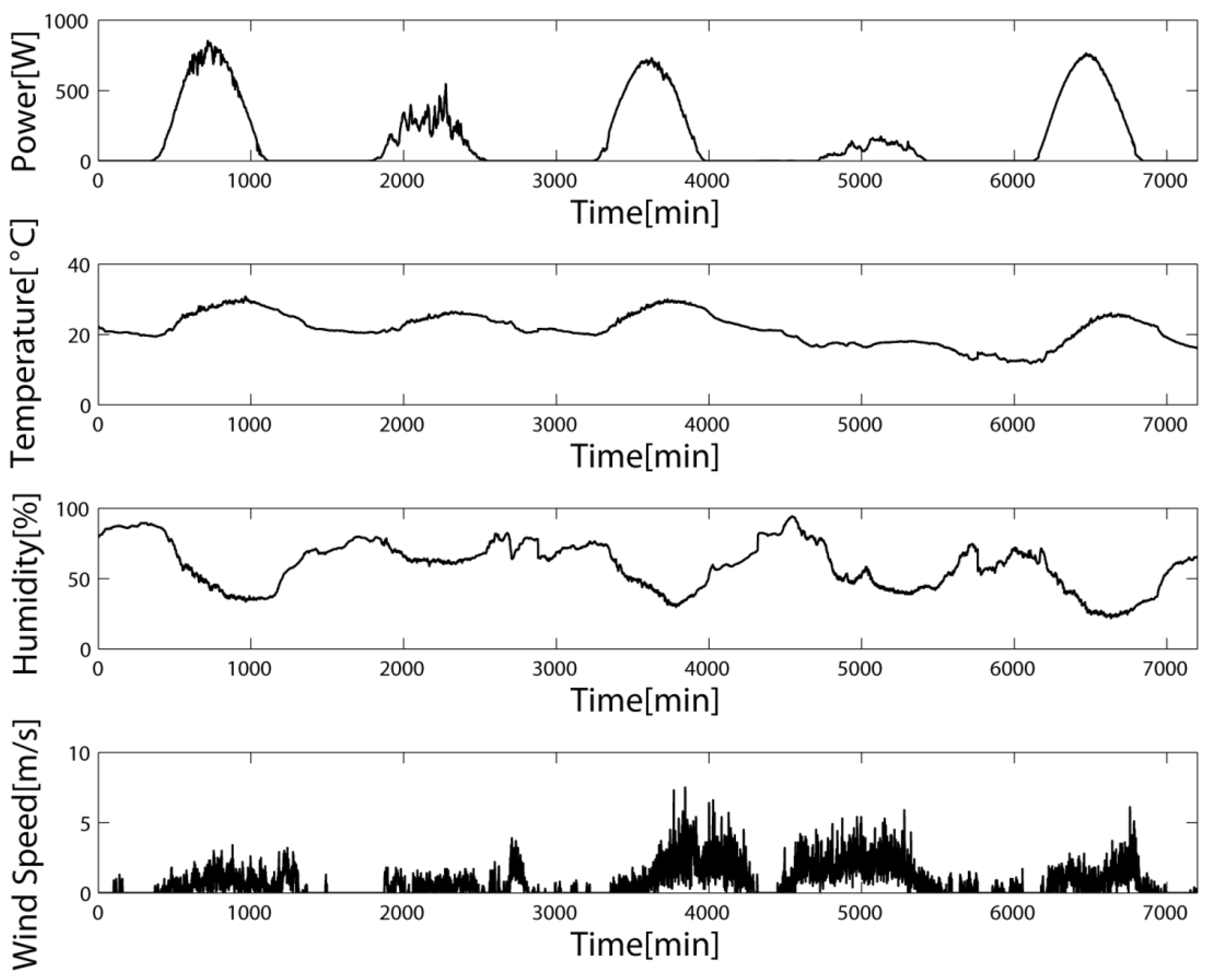
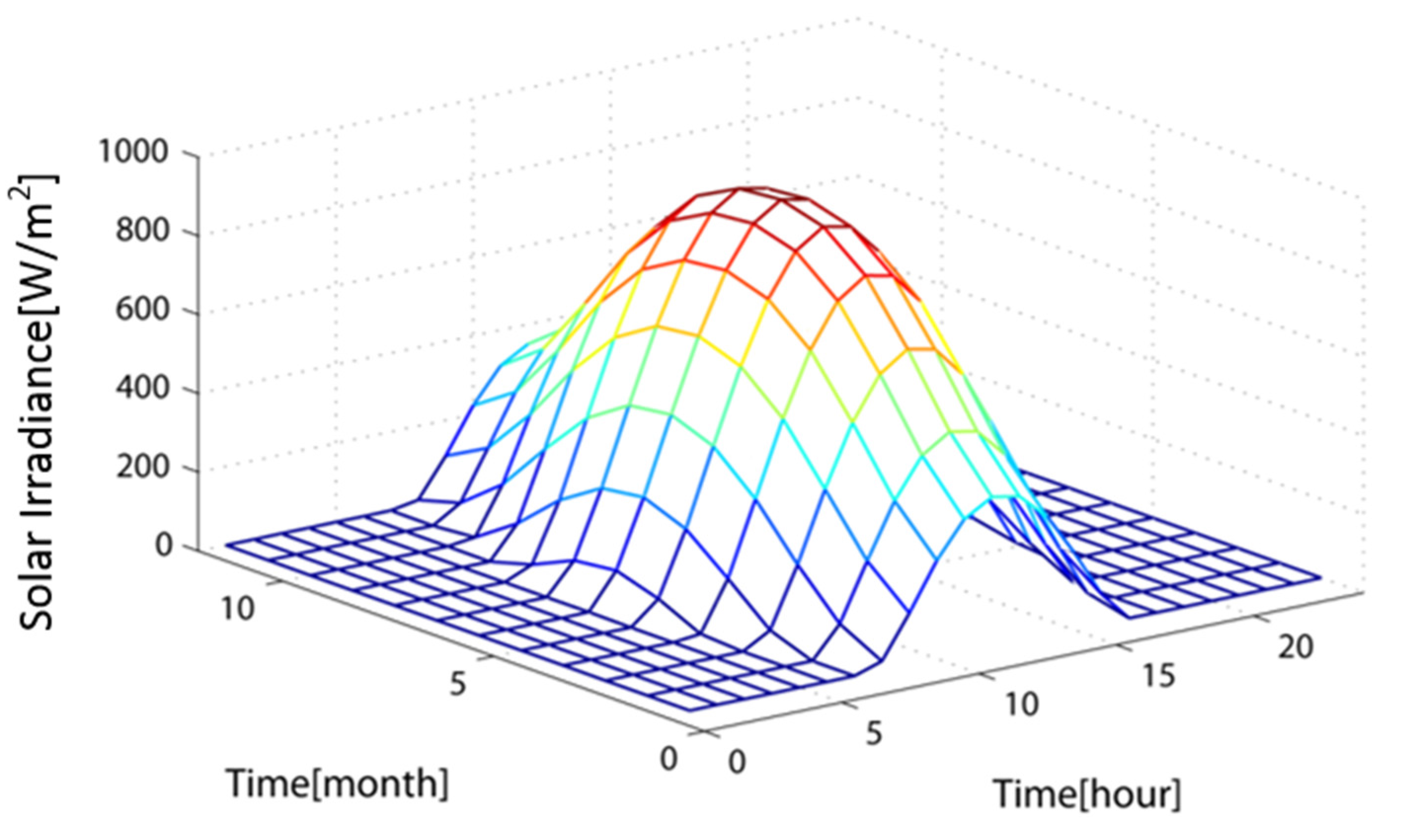
2.1. Periodicity and Non-Stationary Characteristics of Photovoltaic (PV) Output

| Item | Data | Item | Data |
|---|---|---|---|
| Longitude | 116.3059°E | Mounting disposition | Flat roof |
| Latitude | 40.08914°N | Field type | fixed tilted plane |
| Altitude | 80m | Installed capacity | 10 kWp |
| Azimuth | 0° | Technology | polycrystalline silicon |
| Tilt | 37° | PV module | JKM245P |


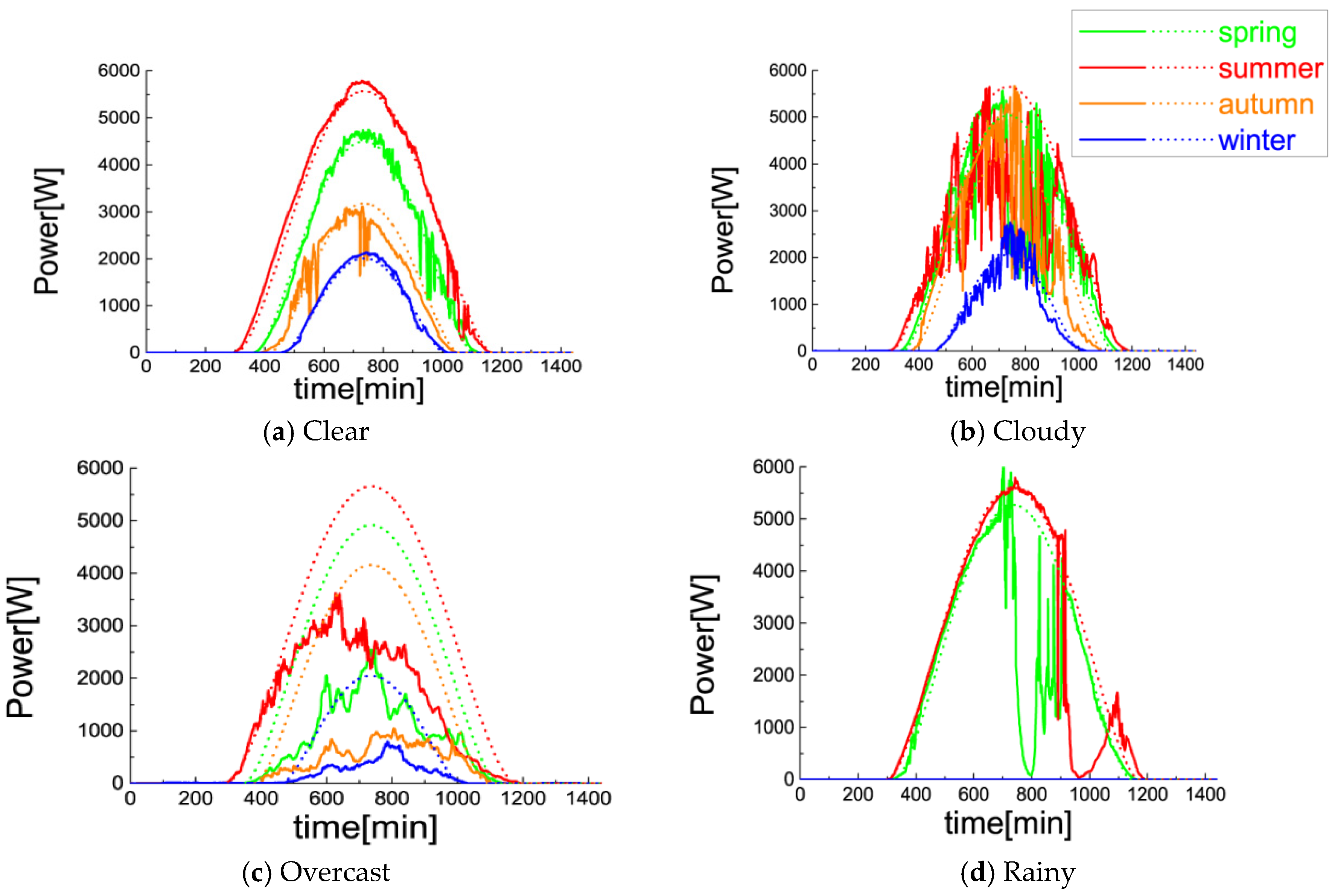
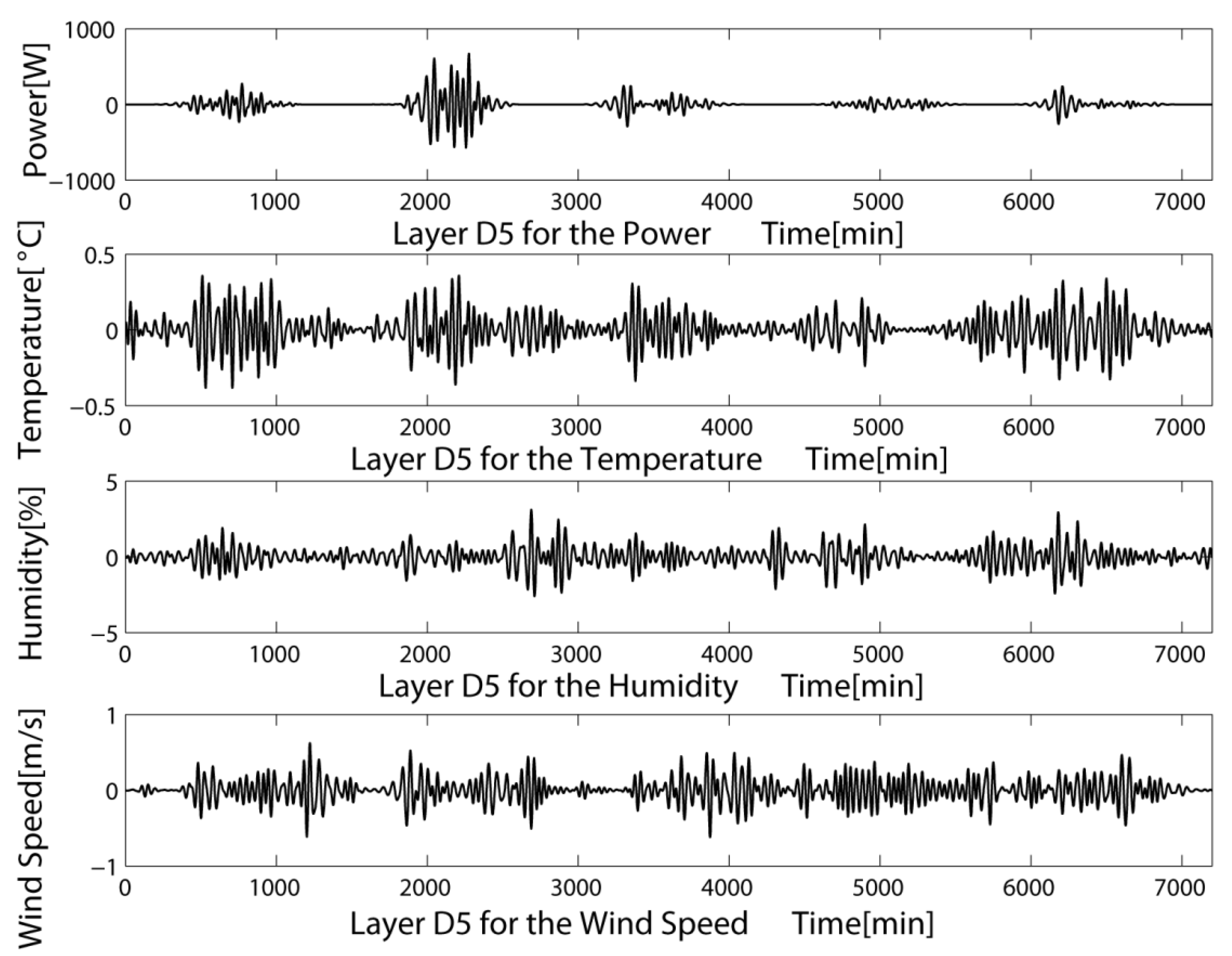
2.2. Influence of Meteorological Factors on Photovoltaic (PV) Output and Model Input Selection
| Weather Condition | Pearson Product-Moment Correlation Coefficient | |||
|---|---|---|---|---|
| Irradiance | Temperature | Humidity | Wind Speed | |
| Clear | 0.966 | 0.322 | −0.527 | −0.229 |
| Cloudy | 0.891 | 0.441 | −0.511 | −0.025 |
| Overcast | 0.987 | 0.409 | −0.478 | 0.125 |
| Rainy | 0.923 | 0.410 | 0.039 | −0.178 |
3. Wavelet Decomposition (WD) for Photovoltaic (PV) Power Output
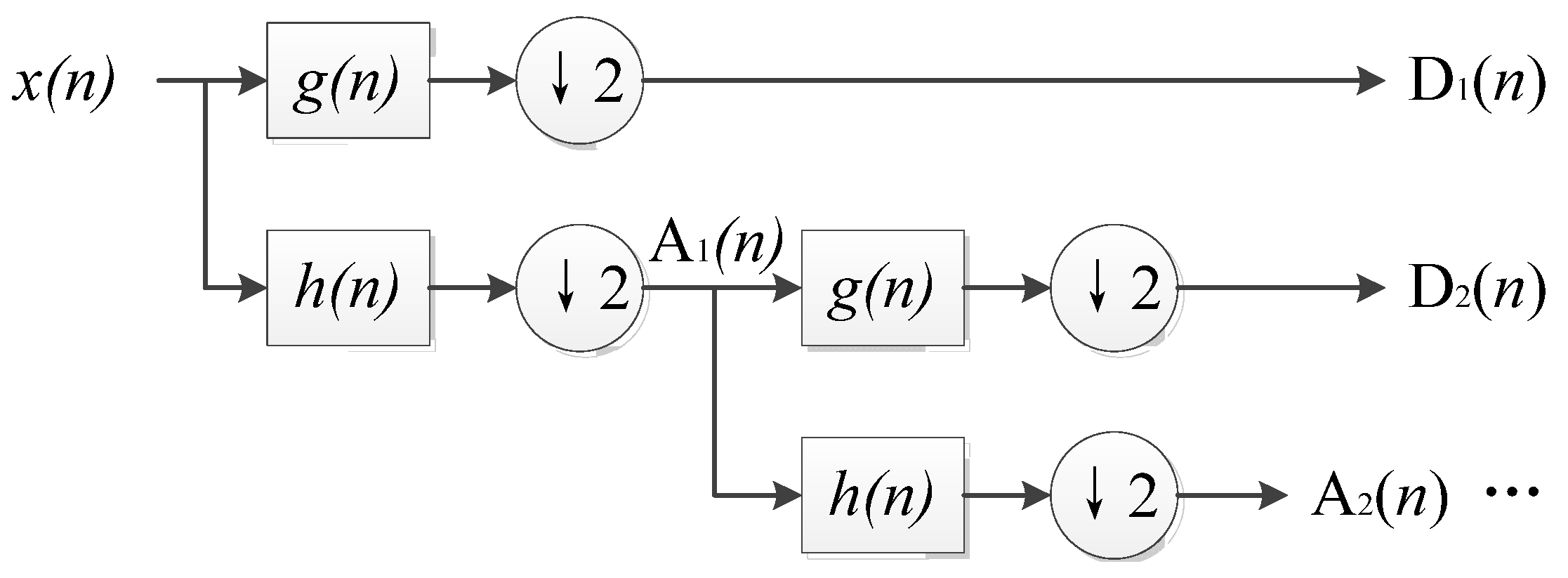
3.1. Wavelet Decomposition (WD) Fundamentals

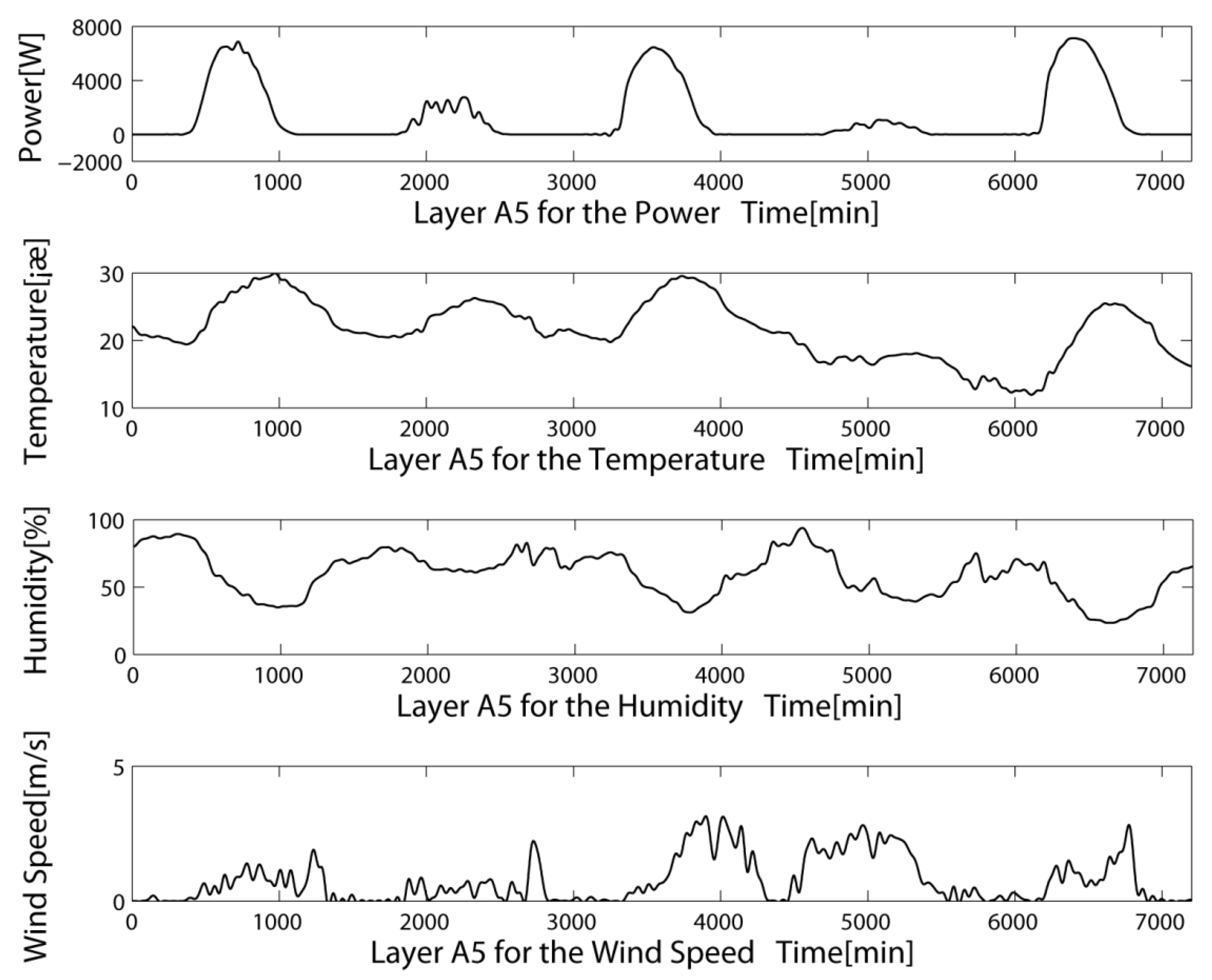
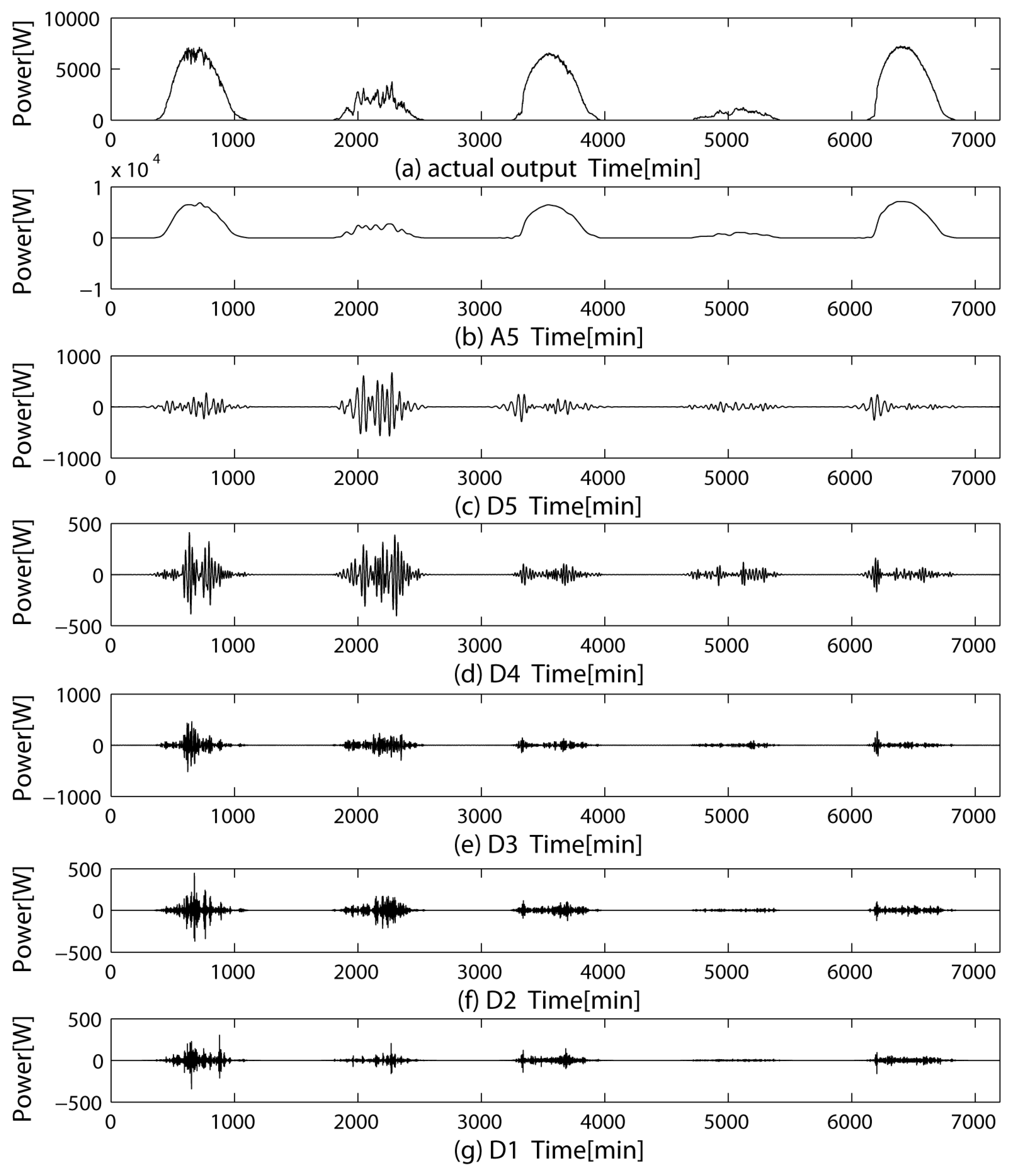
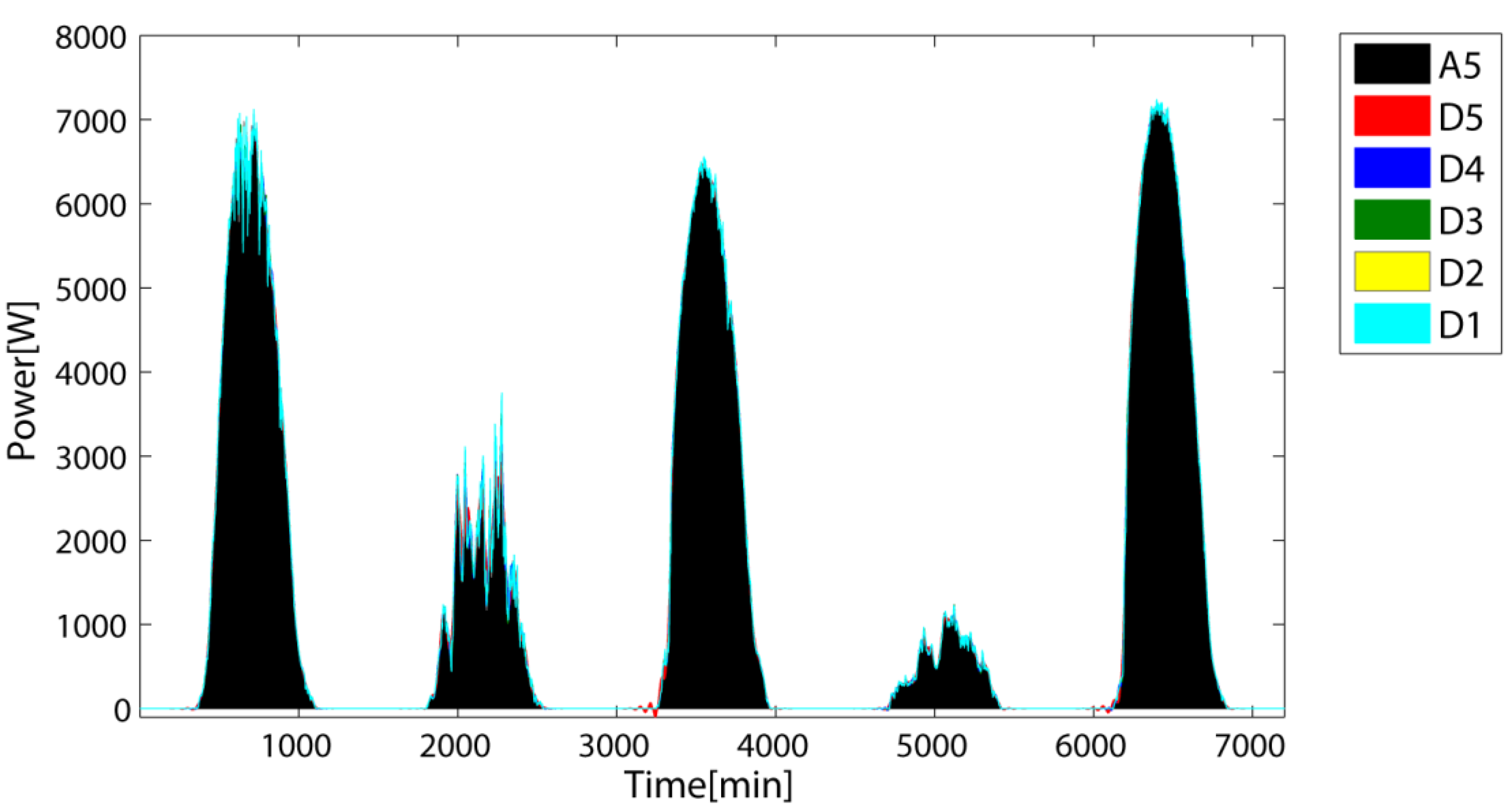
3.2. Wavelet Decomposition (WD) of Power Signals of a Photovoltaic (PV) Power Plant
| Reconstructed Sequence | Definition | Meaning |
|---|---|---|
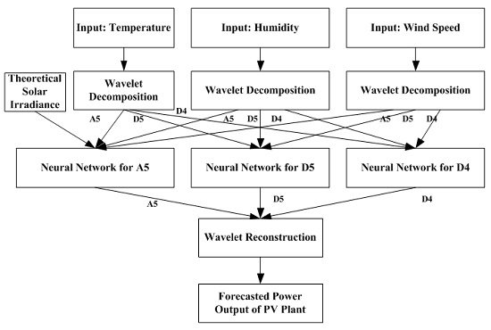
| A5 | smoothed signal at 5th layer | reflects change trend of output power of PV power plant, close to theoretically calculated solar irradiance |
| D5 | detailed signal at 5th layer | reflect composition and change rules of high frequency part of signal |
| D4 | detailed signal at 4th layer | |
| D3 | detailed signal at 3rd layer | |
| D2 | detailed signal at 2nd layer | |
| D1 | detailed signal at 1st layer |
4. Intelligent Forecasting Model Based on Wavelet Decomposition (WD) and Artificial Neural Network (ANN)
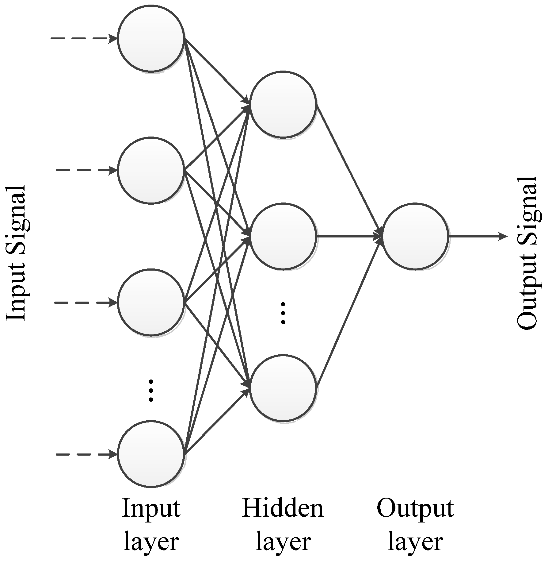
4.1. Artificial Neural Network (ANN) Fundamentals

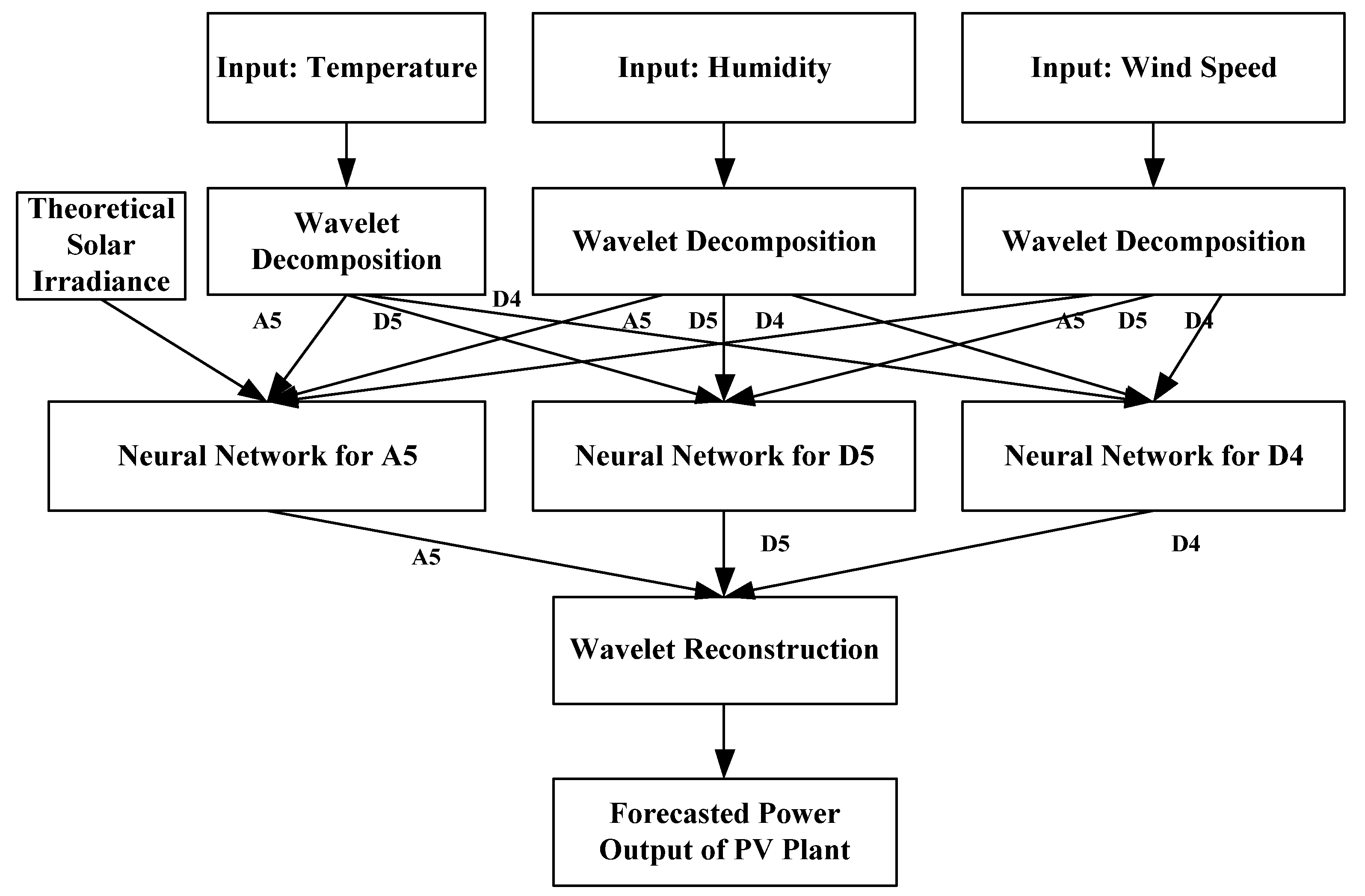
4.2. Forecasting Process


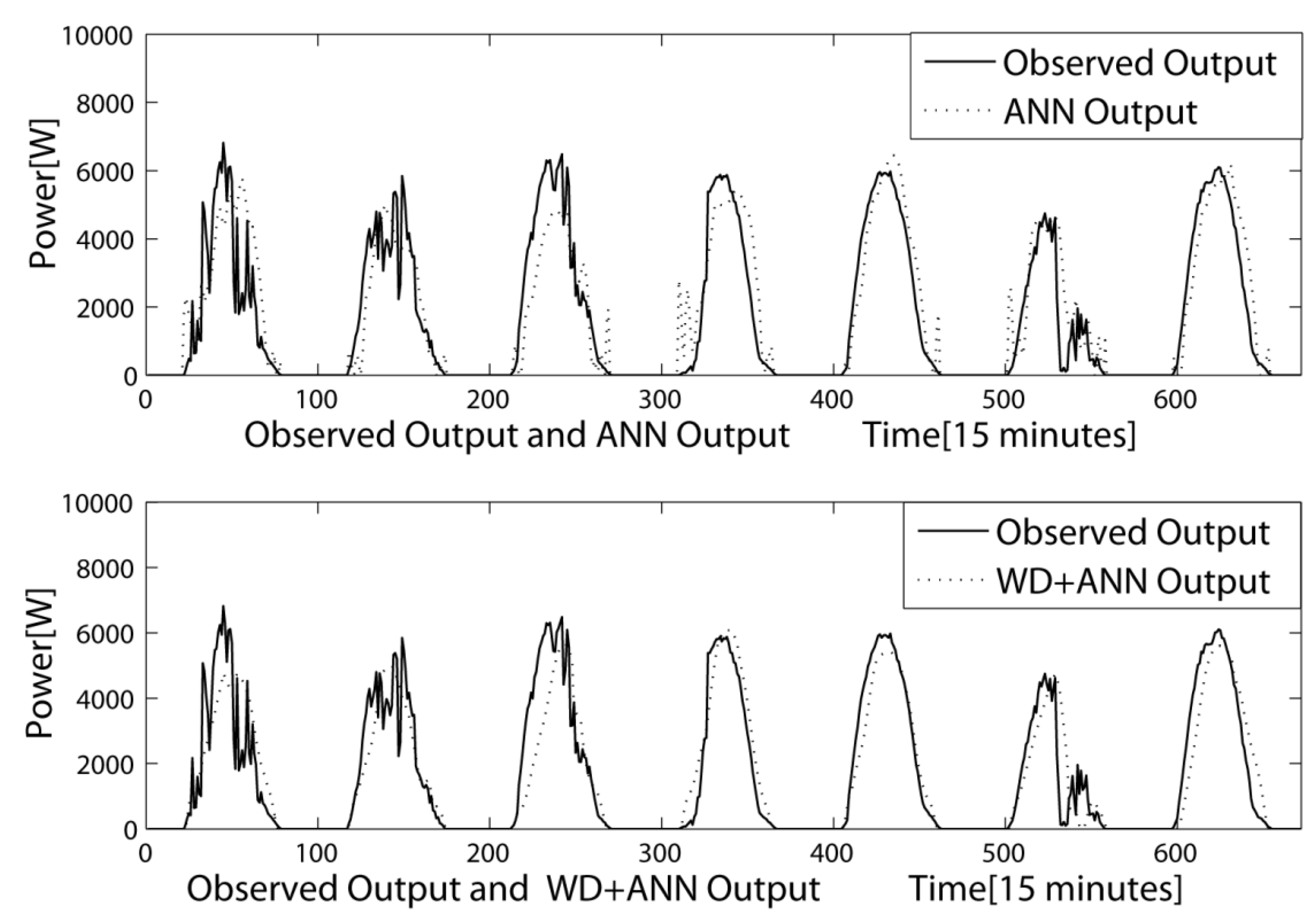
5. Example Analysis and Verification

| Model | Weather | Error | Convergence Epochs | ||
|---|---|---|---|---|---|
| RMSE(%) | MAE(%) | MAPE(%) | |||
| ANN | clear | 9.313 | 4.978 | 13.858 | 4521 |
| cloudy | 18.472 | 10.259 | 21.550 | ||
| overcast | 18.511 | 10.220 | 35.226 | ||
| rainy | 22.948 | 13.062 | 30.926 | ||
| WD + ANN | clear | 7.193 | 3.639 | 9.240 | 2677 |
| cloudy | 16.817 | 9.578 | 21.294 | ||
| overcast | 17.607 | 10.544 | 26.767 | ||
| rainy | 19.663 | 10.349 | 25.373 | ||
6. Conclusions
Acknowledgments
Author Contributions
Conflicts of Interest
Appendix

References
- Mandal, P.; Madhira, S.T.S.; haque, A.U.; Meng, J.; Pineda, R.L. Forecasting power output of solar photovoltaic system using wavelet transform and artificial intelligence techniques. Procedia Comput. Sci. 2012, 12, 332–337. [Google Scholar] [CrossRef]
- Ogliari, E.; Grimaccia, F.; Leva, S.; Mussetta, M. Hybrid predictive models for accurate forecasting in PV systems. Energies 2013, 6, 1918–1929. [Google Scholar] [CrossRef] [Green Version]
- Lorenz, E.; Scheidsteger, T.; Hurka, J.; Heinemann, D.; Kurz, C. Regional PV power prediction for improved grid integration. Prog. Photovolt. 2010, 19, 757–771. [Google Scholar] [CrossRef]
- Lorenz, E.; Heinemann, D.; Kurz, C. Local and regional photovoltaic power prediction for large scale grid integration: Assessment of a new algorithm for snow detection. Prog. Photovolt.: Res. Appl. 2012, 20, 760–769. [Google Scholar] [CrossRef]
- Karthikeyan, L.; Nagesh Kumar, D. Predictability of nonstationary time series using wavelet and EMD based ARMA models. J. Hydrol. 2013, 502, 103–119. [Google Scholar] [CrossRef]
- Mellit, A.; Kalogirou, S.A. Artificial intelligence techniques for photovoltaic applications: A review. Prog. Energy Combust. Sci. 2008, 34, 574–632. [Google Scholar] [CrossRef]
- Pedro, H.T.C.; Coimbra, C.F.M. Assessment of forecasting techniques for solar power production with no exogenous inputs. Sol. Energy 2012, 86, 2017–2028. [Google Scholar] [CrossRef]
- Voyant, C.; Muselli, M.; Paoli, C.; Nivet, M.-L. Numerical weather prediction (NWP) and hybrid ARMA/ANN model to predict global radiation. Energy 2012, 39, 341–355. [Google Scholar] [CrossRef]
- Monteiro, C.; Santos, T.; Fernandez-Jimenez, L.; Ramirez-Rosado, I.; Terreros-Olarte, M. Short-term power forecasting model for photovoltaic plants based on historical similarity. Energies 2013, 6, 2624–2643. [Google Scholar] [CrossRef]
- Mellit, A.; Benghanem, M.; Kalogirou, S.A. An adaptive wavelet-network model for forecasting daily total solar-radiation. Appl. Energy 2006, 83, 705–722. [Google Scholar] [CrossRef]
- Fryzlewicz, P.; van Bellegem, S.; von Sachs, R. Forecasting non-stationary time series by wavelet process modelling. Ann. Inst. Stat. Math. 2003, 55, 737–764. [Google Scholar] [CrossRef] [Green Version]
- Catalão, J.P.S.; Pousinho, H.M.I.; Mendes, V.M.F. Short-term wind power forecasting in Portugal by neural networks and wavelet transform. Renew. Energy 2011, 36, 1245–1251. [Google Scholar] [CrossRef]
- Domingues, M.O.; Mendes, O.; da Costa, A.M. On wavelet techniques in atmospheric sciences. Adv. Space Res. 2005, 35, 831–842. [Google Scholar] [CrossRef]
- Mellit, A.; Pavan, A.M. A 24-h forecast of solar irradiance using artificial neural network: Application for performance prediction of a grid-connected PV plant at Trieste, Italy. Sol. Energy 2010, 84, 807–821. [Google Scholar] [CrossRef]
- Azadeh, A.; Maghsoudi, A.; Sohrabkhani, S. An integrated artificial neural networks approach for predicting global radiation. Energy Convers. Manag. 2009, 50, 1497–1505. [Google Scholar] [CrossRef]
- Chen, S.H.; Jakeman, A.J.; Norton, J.P. Artificial intelligence techniques: An introduction to their use for modelling environmental systems. Math. Comput. Simul. 2008, 78, 379–400. [Google Scholar] [CrossRef]
- Kumar, L.; Skidmore, A.K.; Knowles, E. Modelling topographic variation in solar radiation in a GIS environment. Int. J. Geogr. Inf. Sci. 1997, 11, 475–497. [Google Scholar] [CrossRef]
- Gueymard, C.A. Clear-sky irradiance predictions for solar resource mapping and large-scale applications: Improved validation methodology and detailed performance analysis of 18 broadband radiative models. Sol. Energy 2012, 86, 2145–2169. [Google Scholar] [CrossRef]
© 2015 by the authors; licensee MDPI, Basel, Switzerland. This article is an open access article distributed under the terms and conditions of the Creative Commons by Attribution (CC-BY) license (http://creativecommons.org/licenses/by/4.0/).
Share and Cite
Zhu, H.; Li, X.; Sun, Q.; Nie, L.; Yao, J.; Zhao, G. A Power Prediction Method for Photovoltaic Power Plant Based on Wavelet Decomposition and Artificial Neural Networks. Energies 2016, 9, 11. https://doi.org/10.3390/en9010011
Zhu H, Li X, Sun Q, Nie L, Yao J, Zhao G. A Power Prediction Method for Photovoltaic Power Plant Based on Wavelet Decomposition and Artificial Neural Networks. Energies. 2016; 9(1):11. https://doi.org/10.3390/en9010011
Chicago/Turabian StyleZhu, Honglu, Xu Li, Qiao Sun, Ling Nie, Jianxi Yao, and Gang Zhao. 2016. "A Power Prediction Method for Photovoltaic Power Plant Based on Wavelet Decomposition and Artificial Neural Networks" Energies 9, no. 1: 11. https://doi.org/10.3390/en9010011