4.1. Method of Experiment
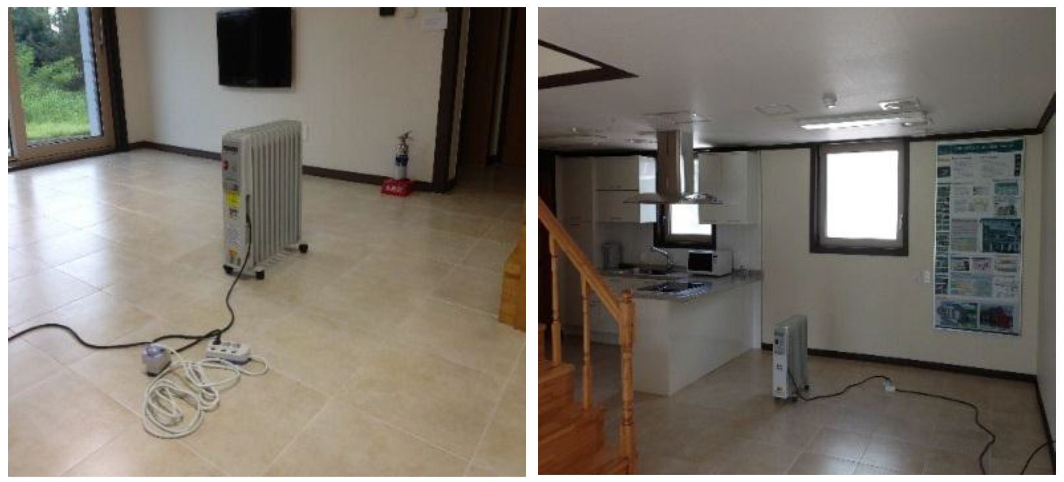
Experimental tests were conducted in August and March at the demonstration house for space cooling and heating modes to evaluate the effectiveness of the thermal storage control methods. Because, in the demonstration house, there was no occupant during the test, two electric heaters were placed in the living room and near the kitchen space of the first floor to simulate the internal heat gains of residential buildings. The heater in the living room was scheduled to turn on each hour for 15 min at a 1 kW electric input to generate roughly 250 Wh of internal heat gain per hour [
13]. The heater was operated from 6 am to 7 pm. Another electric heater was placed near the kitchen to simulate the internal heat gain from cooking by turning on the heater for 30 min at 7 am, 11 pm, and 5 pm. The electric heaters were not used for heating operation mode tests.
Figure 5 shows the electric heaters used for cooling-mode tests.
Figure 5.
Two electric heaters on the first floor inside the demonstration house to simulate internal heat gains.
Figure 5.
Two electric heaters on the first floor inside the demonstration house to simulate internal heat gains.
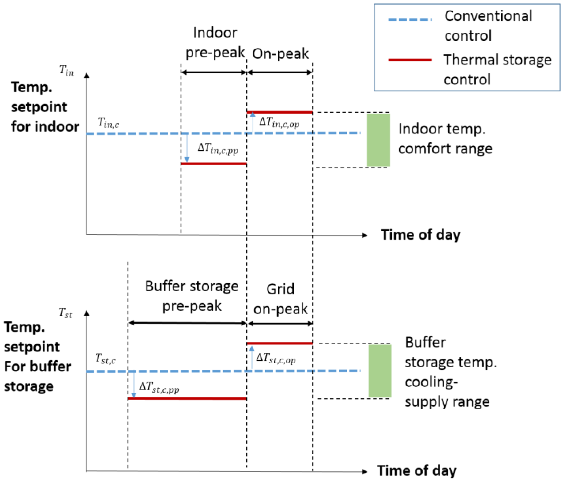
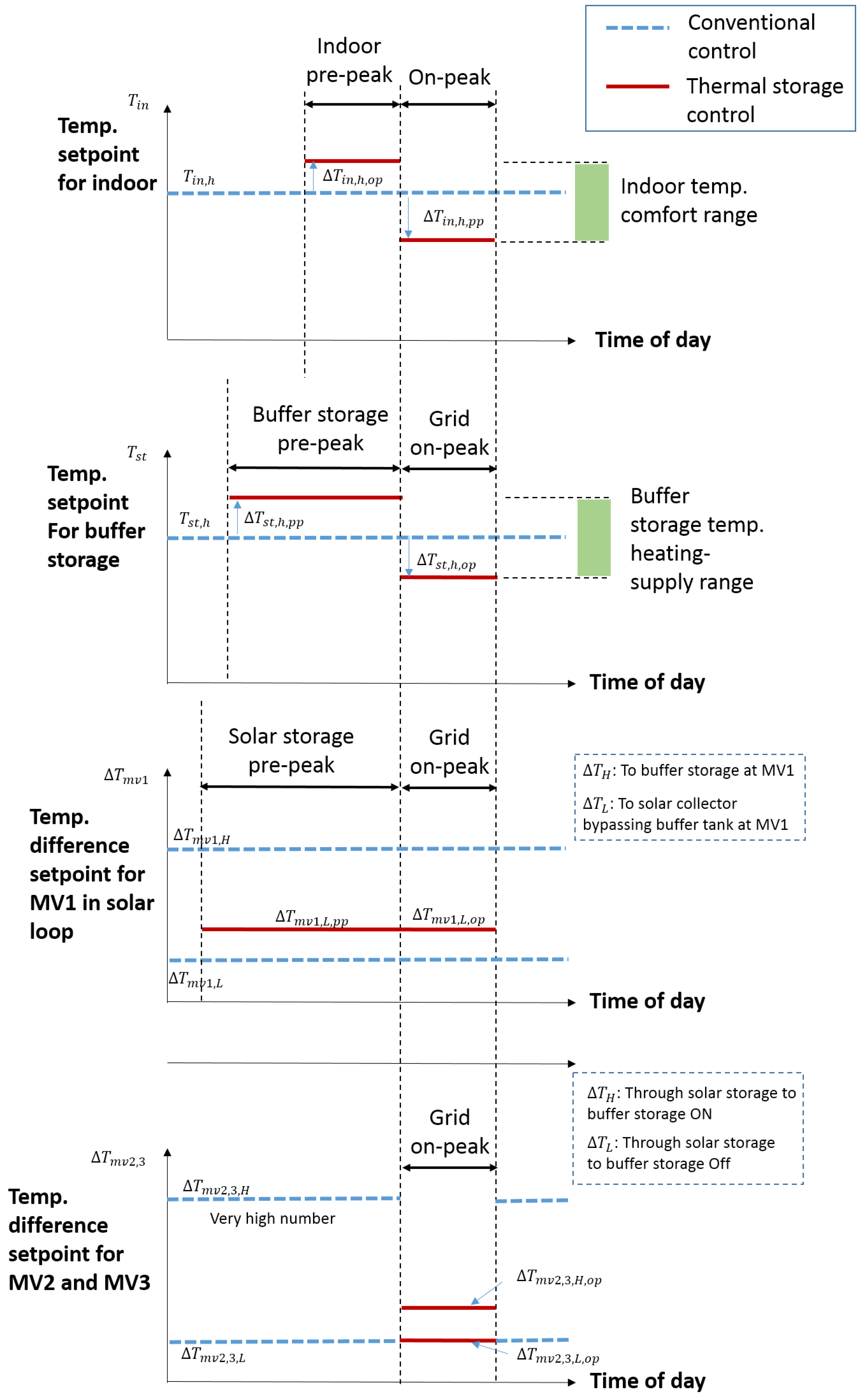
The adjustments of the setpoints for the indoor space are performed by changing the setpoints of the thermostats in each room. The setpoint for buffer thermal storage is changed on the control display panel of the heat pump. All adjustments were performed manually. For the cooling test in the conventional control, Tin,c was 26 °C and Tst,c was 12 °C, with an upper deadband of 3 °C for the whole day. For thermal storage control, ΔTin,c was 2 °C, ΔTpp,c was 2 °C with an upper deadband of 1 °C, and ΔTop,c was 8 °C with an upper deadband of 1 °C. For the heating test, in the conventional control, Tin,h was 28 °C and Tst,h was 45 °C with an upper deadband of 2 °C for the whole day. For thermal storage control, ΔTin,h was 2 °C, ΔTpp,h was 0 °C with an upper deadband of 1 °C, and ΔTop,h was 8 °C with an upper deadband of 2 °C. It should be noted that the indoor heating temperature setpoint was set higher than the normal temperature setpoint of 21 to 23 °C because the heating test was conducted on days that were not so cold in March. In conventional control of motor valve MV1, ΔTmv1,H and ΔTmv1,L were set to 12 °C and 3 °C, respectively, and ΔTmv1,L,pp and ΔTmv1,L,op were increased to 15 °C in order to bypass the buffer storage tank when solar heat is collected. For conventional control of motor valves MV2 and MV3, ΔTmv23,H and ΔTmv23,L were set to 50 °C which is very high value and 3 °C, respectively; ΔTmv23,H,op was set to 10 °C.
The chilled water pump for space cooling was always on during the test to investigate the temperature variation of the chilled water in the buffer storage tank. However, the electric power consumption of the chilled water pump is assumed to be synchronized to the operation status of the FCU, which is a reasonable approach when simulating the actual situation.
The measurement and data acquisition system logs solar radiation, outdoor temperature, indoor temperatures, and water temperature in the buffer storage tank; inlet and outlet flow temperatures of the heat pump; inlet and outlet temperatures of the buffer storage tank; power consumption of the FCU, heat pump, and its associated components; power generated by the solar PV system; and flow rate of the chilled water from the heat pump, which is used for space cooling. All data was recorded using a data logger and a computer at a time interval of 1 min. The water temperature was measured using a four-wire RTD (resistance temperature detector) sensor; the indoor air temperatures were measured using calibrated thermocouple sensors. The flow rates of the chilled water from the heat pump and from the buffer storage tank were measured once using an electro-magnetic flow meter; thereafter, it was assumed that the flow rate was constant. The operation status of each pump was recorded to estimate the electricity consumption. The measuring points for the indoor temperatures in each room were located two meters above the floor; however, this seems quite high to evaluate the indoor thermal environment. Therefore, the measured indoor temperature data were modified based on the temperature difference from the temperature measured near the thermostat using a well-calibrated temperature sensor.
4.2. Experimental Results
Experiments were performed in August and March for space-cooling and space-heating mode tests, respectively. After the tests, three test days with similar weather conditions were selected from the cooling-mode test days to compare the energy saving performance of the three different control strategies, i.e., BSC and CSC with CC. Similarly, two test days with similar weather conditions were selected for the heating-mode test to evaluate the two control strategies, i.e., CC and CSC.
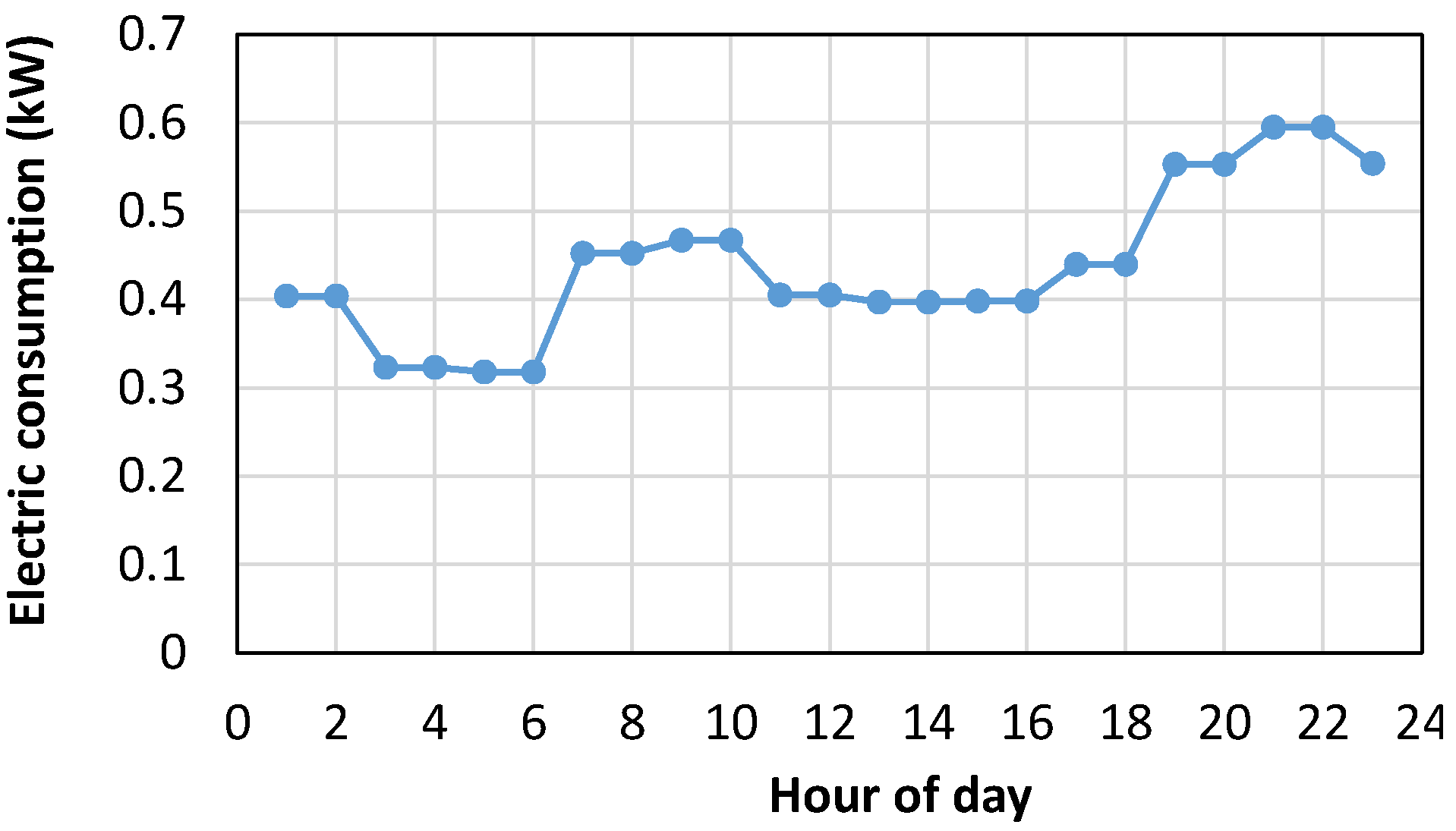
To evaluate the impact on the electricity consumption of the house, the energy consumption of the air-conditioning system was measured; however the electricity consumption of the house for lighting and plug loads was approximated, as seen in
Figure 6 [
14]. This profile was obtained based on electricity consumption data measured in six apartments in high-rise residential building complexes [
14].
Figure 7 and
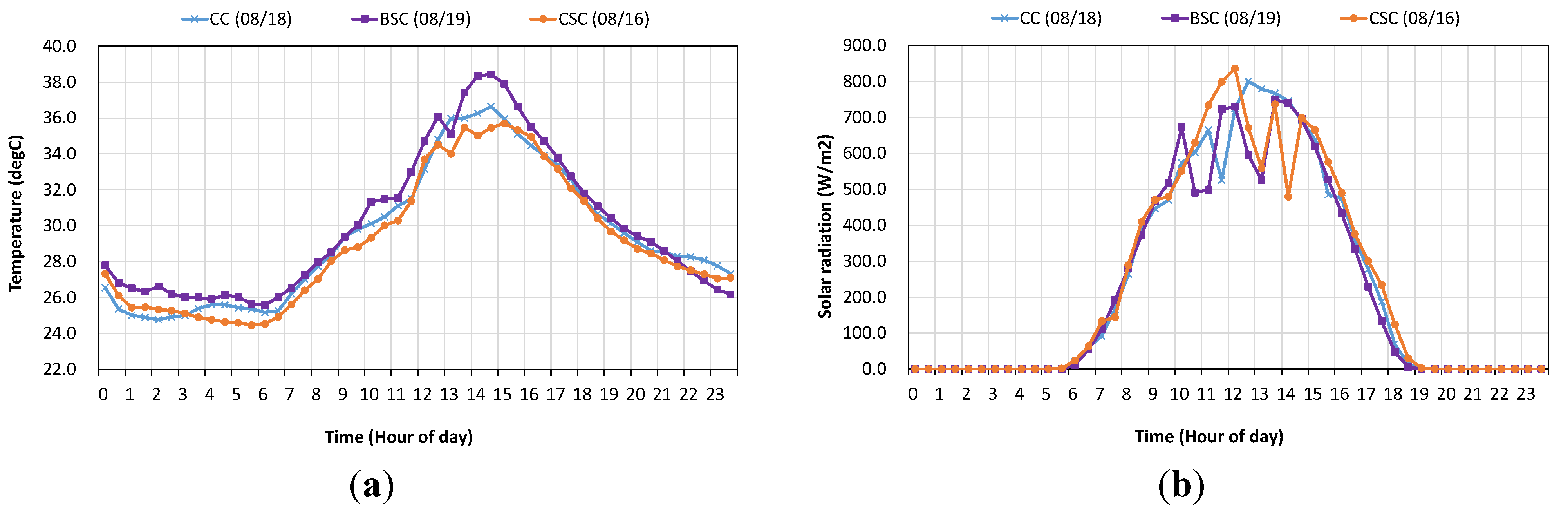
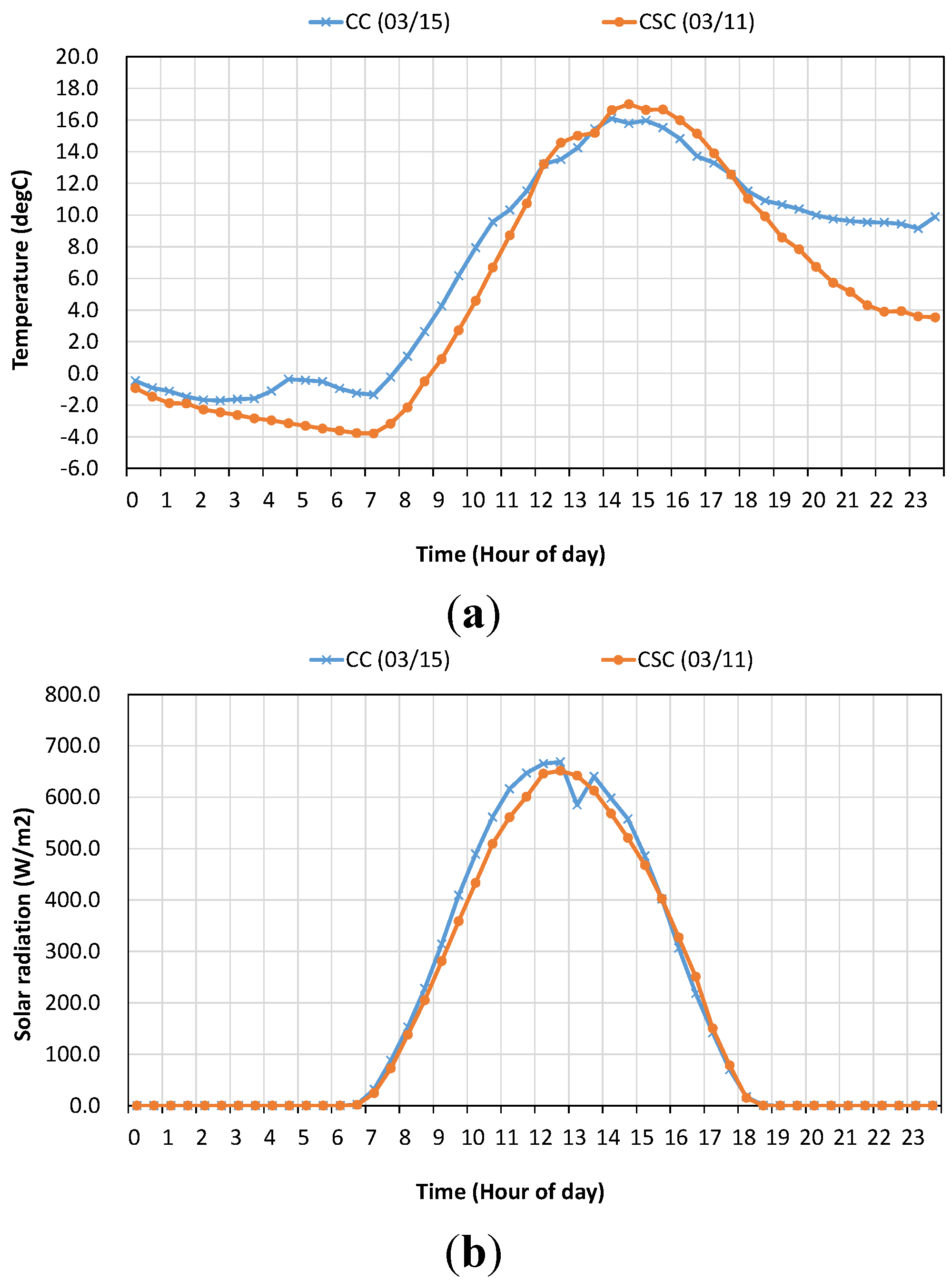
Figure 8 compare the outdoor temperature and the horizontal solar radiation for the three selected days for space-cooling mode tests and two selected days for space-heating mode tests. Regarding the similarity of the weather conditions between the compared test days, the root-mean squared differences for the three days are below 10% and 3% for solar radiation and ambient temperature, respectively. In fact, we found that the highest national grid peak demand in August of 2013 happened on the day in which the BSC strategy was tested. The peak demand was 7401.5 MW with a 6.4% reserve margin rate [
15]. The day of the week was Monday. On the CSC test day, the national grid had a similar peak demand of 7321.6 MW. The peak demand on the test day with CC was much lower, at 6271.0 MWh, because it was a Sunday. The test days for space-heating mode occurred in March; therefore, national grid peak demand did not occur during the test days.
Figure 6.
Approximated electricity load profile of other usage for one day (comprising lighting and plug load).
Figure 6.
Approximated electricity load profile of other usage for one day (comprising lighting and plug load).
Figure 7.
Comparison of weather conditions, (a) outdoor temperature and (b) global horizontal solar radiation, for three space-cooling operation test days with CC, BSC, and CSC.
Figure 7.
Comparison of weather conditions, (a) outdoor temperature and (b) global horizontal solar radiation, for three space-cooling operation test days with CC, BSC, and CSC.
Figure 8.
Comparison of weather conditions, (a) outdoor temperature and (b) global horizontal solar radiation, for two space-heating operation test days with CC and CSC.
Figure 8.
Comparison of weather conditions, (a) outdoor temperature and (b) global horizontal solar radiation, for two space-heating operation test days with CC and CSC.
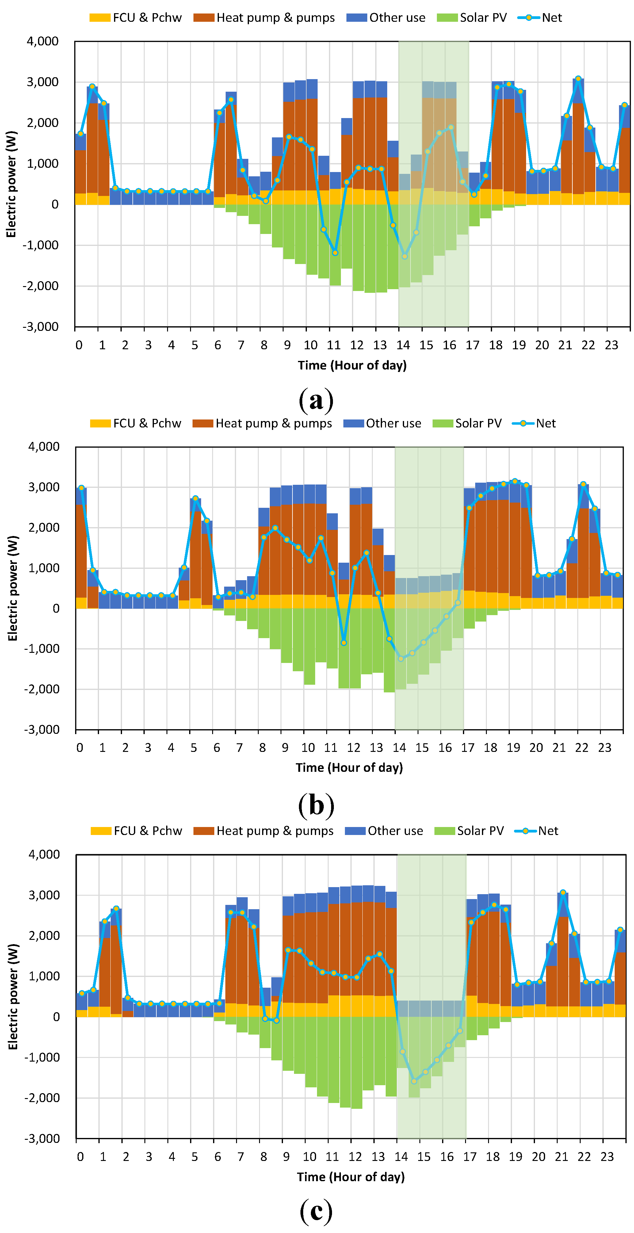
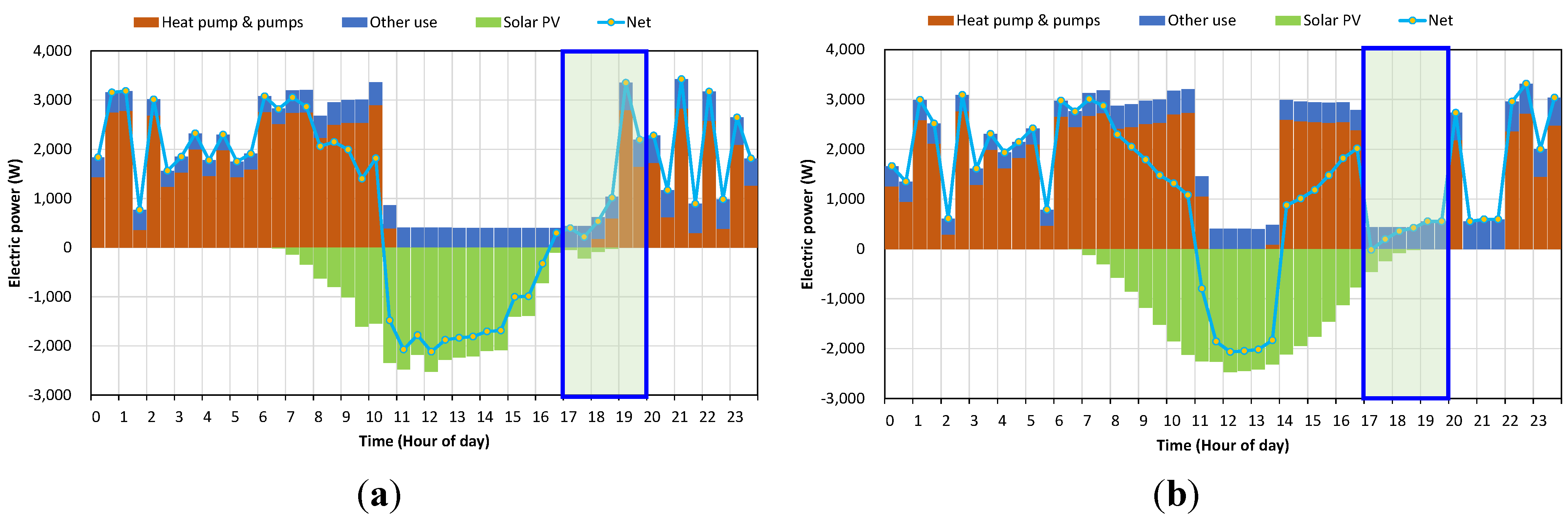
Figure 9 represents the net electricity consumption of the three different control strategies for cooling-mode tests with average values for 30-min intervals.
Table 3 presents electricity consumption during the peak period for the three control strategies.
Table 4 compares similar results regarding electricity consumption for the whole test day. “FCU & Pchw” indicates electricity consumption of the FCU and the chilled water circulation pump. “Heat pump and pumps” indicates the electricity consumption of the heat pump, the fluid circulation pump between the heat pump and the ground heat exchanger, and the fluid circulation pump between the heat pump and the buffer storage. The electricity generation from the solar PV system is negative in the figures so that the net electricity consumption can be negative if the PV generation exceeds the total electricity consumption.
As shown in
Figure 9a, the net electric power consumption with CC during the peak period from 2 pm to 5 pm was negative for 1 h, from 2 pm to 3 pm, and became positive for the remaining 2 h, from 3 pm to 5 pm. Due to the nearly cyclic power demand of the heat pump system, the power demand alternates with a period of 3–4 h. The net electricity consumption during the peak period is 1.77 kWh, with a total electricity consumption of 6.15 kWh and a solar power generation of 4.38 kWh. The net energy consumption with BSC, as seen in
Figure 9b, maintains a negative value except during the last 30 min, at 0.15 kW, from 4:30 pm to 5 pm during the peak period. Because of the subcooling of the buffer storage prior to the peak period, the electricity consumption of the heat pump increased much more than that with CC from 9 am to 2 pm. The heat pump did not run during the peak period; however, the FCU was running throughout the peak period. It was observed that the FCU power consumption increased gradually during the peak period. The temperature in the buffer storage tank increased slowly in the range between the lower setpoint and the higher setpoint because the setpoint for the buffer storage tank was set to 20 °C at 2 pm, from 10 °C at 9 am. As the temperature of the chilled water in the buffer storage tank rises, the FCU in each room requires more cool air supply to meet the indoor setpoint, resulting in a longer FCU operation time. The net energy consumption during the peak period with BSC, seen in
Table 3, is negative, at −1.90 kWh, with a total electricity consumption of 2.41 kWh and a solar power generation of 4.30 kWh. As seen in
Figure 9b, the net power demand during the peak period had its lowest value at the onset time of the peak,
i.e., at 2 pm; then it gradually increased toward the end of the peak period. It was observed that the shape of the net power demand curve is affected by the shape of the generated power curve, because the electricity demand of the house is significantly reduced in BSC while the power generated by the solar PV system is high. For CSC, the net energy consumption seen in
Figure 9c is negative throughout the peak period. Because of the subcooling and precooling requirements prior to the peak period, the electricity use of the heat pump increased much more than with CC or BSC. However, it should be noted that neither the heat pump nor the FCU ran during the peak period. Because the building thermal mass was cooled by precooling before the peak period, the cooling demand of the FCU and buffer storage during the peak period was reduced to zero in this case. This means that the indoor space temperature stayed below the setpoint (28 °C) until the end of the peak period, otherwise the FCU would have turned on during the peak period. The net energy consumption with CSC during the peak period presented in
Table 3 is −2.92 kWh, with a total energy consumption of 1.19 kWh and a solar power generation of 4.15 kWh. This means that the electricity production from the house exceeded the electricity consumption of the house, and therefore, it supplied excess electricity to the grid during the peak period. It should also be noted that the operating time of the heat pump increased by 2 and 4 h after the peak period with CSC and BSC, respectively, compared to CC. The reason that the operating time of the heat pump after the peak period with BSC is longer than that with CSC is that the water temperature is higher in the buffer storage tank in BSC. The increased thermal load due to precooling of the building thermal mass is transferred to the buffer storage tank before the peak period, resulting in higher energy consumption by the heat pump in CSC than in BSC. This phenomenon reduced the operating time of the heat pump after the peak period in CSC. The energy consumption of the cooling system for the whole day, presented in
Table 4, is roughly 23.3 to 23.5 kWh, which is not significantly different for different control strategies. This result, however, proves that the thermal storage control of the buffer storage and the building thermal mass does significantly reduce the cooling energy consumption during the peak period without sacrificing electricity consumption for the whole day.
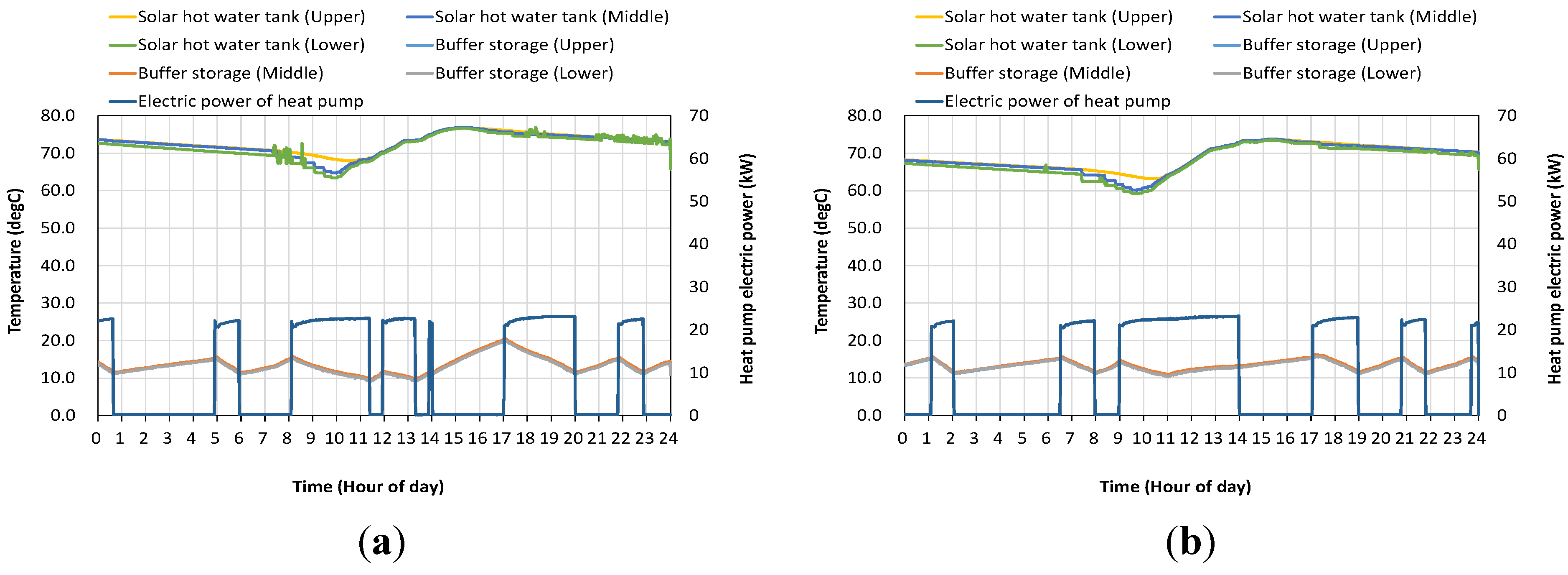
Figure 10 shows temperatures in the solar hot water tank and the buffer storage tank, and the heat pump electric power in BSC and CSC. The temperature in the buffer storage decreases from 9 am to 11 am, and then, increases until 2 pm, because the indoor setpoints were adjusted to a lower comfort limit temperature for precooling. During the on-peak period, the temperature increases more rapidly in the case of BSC, compared to CSC, both because there was no precooling in BSC control and because some of the FCU units should run when the indoor temperature reaches the indoor setpoint during on-peak period, which does not happen in CSC control.
Figure 9.
Energy consumption for different control strategies (a) CC; (b) BSC; and (c) CSC in space-cooling operation mode tests.
Figure 9.
Energy consumption for different control strategies (a) CC; (b) BSC; and (c) CSC in space-cooling operation mode tests.
Table 3.
Electricity consumption during on-peak period with three different control strategies for space-cooling-mode tests.
Table 3.
Electricity consumption during on-peak period with three different control strategies for space-cooling-mode tests.
| (Unit: kWh) | CC | BSC | CSC |
|---|
| Energy consumption | Energy consumption | Energy saving (%) | Energy consumption | Energy saving (%) |
|---|
| Heat pump and pumps | 3.90 | 0.00 | 100.00 | 0.00 | 100.00 |
| FCU and PCHW | 1.05 | 1.21 | −15.24 | 0.00 | 100.00 |
| Cooling sum | 4.95 | 1.21 | 75.56 | 0.00 | 100.00 |
| Other use | 1.19 | 1.19 | 0.00 | 1.19 | 0.00 |
| Total sum | 6.15 | 2.41 | 60.81 | 1.19 | 80.65 |
| Solar PV | −4.38 | −4.30 | 1.83 | −4.15 | 5.25 |
| Net sum | 1.77 | −1.90 | 207.34 | −2.95 | 266.67 |
Table 4.
Electricity consumption for the whole day for three different control strategies for space-cooling-mode tests.
Table 4.
Electricity consumption for the whole day for three different control strategies for space-cooling-mode tests.
| (Unit: kWh) | CC | BSC | CSC |
|---|
| Energy consumption | Energy consumption | Energy saving (%) | Energy consumption | Energy saving (%) |
|---|
| Heat pump and pumps | 23.44 | 23.30 | 0.60 | 23.49 | −0.21 |
| FCU and PCHW | 6.23 | 6.32 | −1.44 | 5.67 | 8.99 |
| Cooling sum | 29.66 | 29.62 | 0.13 | 29.16 | 1.69 |
| Other use | 10.38 | 10.38 | 0.00 | 10.38 | 0.00 |
| Total sum | 40.04 | 40.00 | 0.10 | 39.54 | 1.25 |
| Solar PV | −15.60 | −14.67 | 5.96 | −15.68 | −0.51 |
| Net sum | 24.44 | 25.33 | −3.64 | 23.86 | 2.37 |
Figure 10.
Temperature variation in solar hot water tank and buffer storage tank, and heat pump electric power for cooling operation mode test using (a) BSC and (b) CSC.
Figure 10.
Temperature variation in solar hot water tank and buffer storage tank, and heat pump electric power for cooling operation mode test using (a) BSC and (b) CSC.
Figure 11 presents the net electricity consumption of the two different control strategies for the heating-mode test with average values at 30min intervals. As shown in
Figure 11a, the net electric power consumption with CC during the peak period from 5 pm to 8 pm gradually increased, and the peak occurred around 7 pm. The net electricity consumption during the peak period was 3.84 kWh with a total electricity consumption of 4.04 kWh and a solar power generation of 0.20 kWh. The net energy consumption with CSC, as seen in
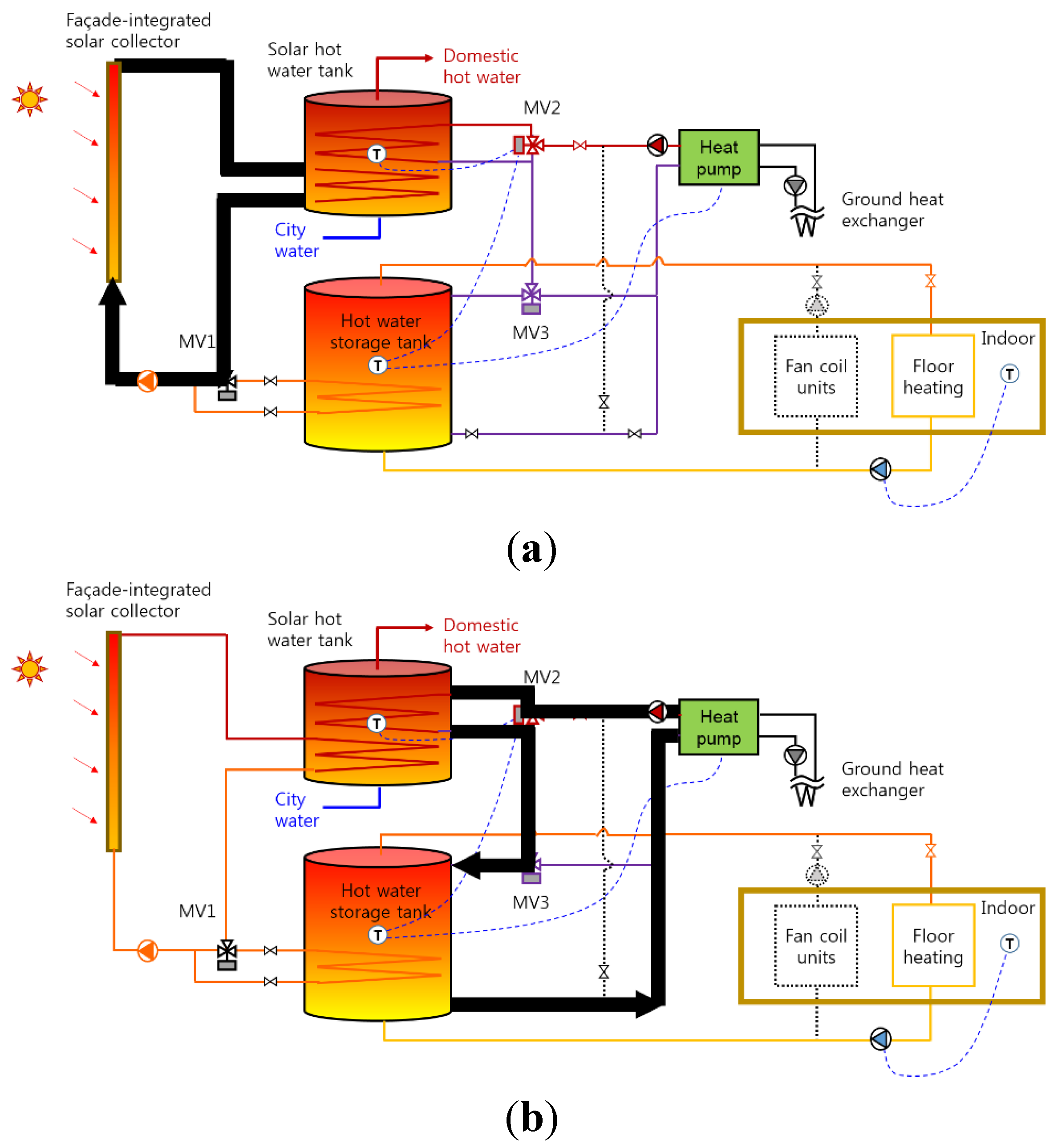
Figure 11b, was maintained near zero during the peak period. Because of the heating requirements of the heat pump prior to the peak period, similar to in the cooling test, the electricity consumption of the heat pump for heating water in the buffer storage increased much more than that with CC. The heat pump did not heat water in the buffer storage during the on-peak period. Hot water from a solar storage tank was also supplied to the buffer storage at the beginning of the on-peak period so as to raise the temperature in the upper part of the buffer storage tank. This can provide another benefit, by reducing the likelihood of heat pump operation during the on-peak period.
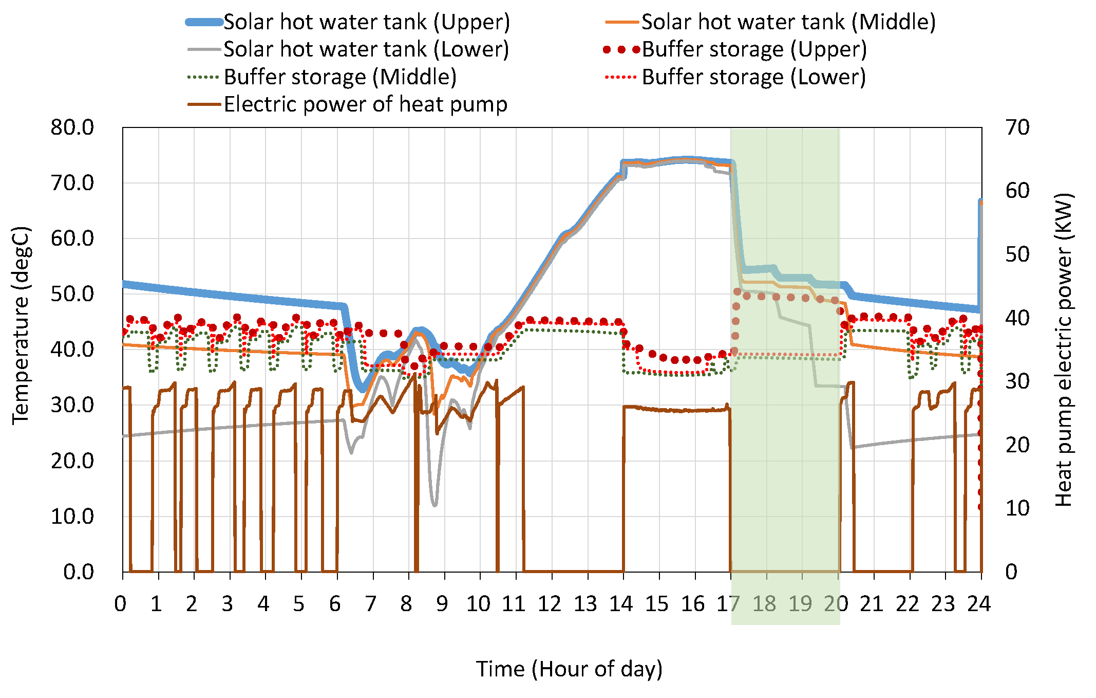
Figure 12 shows the water temperatures in the solar hot water tank and the buffer storage tank and the electric power of the heat pump in CSC in a space-heating-mode test. The temperature in solar hot water tank increases rapidly prior to the peak period; it maintains a temperature at the allowable high limit temperature, around 75 °C, and then, reduces the temperature rapidly from the beginning of the on-peak period, because the flow circulating between the solar hot water tank and the buffer storage tank was initiated to supply thermal energy stored in the solar hot water tank to the buffer storage tank, resulting in an increase in temperature in the upper part of the buffer storage tank. As seen in
Figure 11b, the net power demand during the peak period falls to its lowest value at the onset time of the peak at 5 pm, and then, slowly rises until the end of the peak period. It was observed that the shape of the net power demand curve is not strongly affected by the shape of the generated power curve, because the electricity demand of the house is significantly reduced when using CSC, whereas the power generated by the solar PV system is negligible during the on-peak period. The net energy consumption with CSC during the peak period is 1.02 kWh, with a total energy consumption of 1.43 kWh and a solar power generation of 0.41 kWh.
Figure 11.
Electricity consumption for different control strategies (a) CC and (b) CSC in space-heating operation mode tests.
Figure 11.
Electricity consumption for different control strategies (a) CC and (b) CSC in space-heating operation mode tests.
In order to evaluate the impact of building thermal mass of the house on thermal demands after the storage control test, the electric energy consumed by the heat pump was compared overnight for 7 h. The results obtained—13,259 Wh in conventional control and 13,488 Wh in thermal storage control—Did not show a significant difference between conventional control and thermal storage control.
Table 5,
Table 6 and
Table 7 summarize the electricity consumption and peak demand for the cooling and heating tests to compare the control strategies that use thermal storage to the conventional strategy. Negative energy savings means that the electricity consumption in thermal storage control is larger than that with conventional control. The net electricity consumption for the whole day showed quite different results for space-cooling and space-heating tests. The total energy consumption for the whole test day with BSC and CSC control for cooling mode was only marginally different from that observed for conventional control in the cooling test; however, it was roughly 12% higher in the heating test. However, compared to conventional control, the energy consumption during the on-peak period with CSC control was reduced by roughly 80% and 64% in the cooling and heating tests, respectively. Compared to conventional control, peak demand was also significantly reduced (86% and 83% in the cooling and heating test, respectively) when CSC control was adopted. If the impact of the solar PV electricity generation on the electricity consumption and peak demand of the building is considered in the cooling test, the energy savings are further increased. In the heating test, the solar radiation received during the on-peak period was not significant; therefore, the impact of the solar PV module was not as large as in the cooling test. The on-peak period for the heating test was assumed to occur in the late afternoon. It should also be noted that the solar radiation received was not exactly the same on the two test days, and therefore, the solar electricity generated on each day was slightly different.
Figure 12.
Temperature variation in solar hot water tank and buffer storage tank, and heat pump electric power for space-heating operation mode test with CSC.
Figure 12.
Temperature variation in solar hot water tank and buffer storage tank, and heat pump electric power for space-heating operation mode test with CSC.
Table 5.
Comparison of electricity consumption and peak demand for two test days using conventional and peak reduction control strategies in space-cooling-mode tests(BSC in space cooling mode).
Table 5.
Comparison of electricity consumption and peak demand for two test days using conventional and peak reduction control strategies in space-cooling-mode tests(BSC in space cooling mode).
| | Control strategy | CC | BSC | Saving (%) |
|---|
| Energy consumed during the day (kWh/day) | Without PV | 40.04 | 40.00 | 0.10 |
| With PV | 24.44 | 25.33 | −3.64 |
| Energy consumed during on-peak time (kWh/on-peak) | Without PV | 6.15 | 2.41 | 60.81 |
| With PV | 1.77 | −1.90 | 207.34 |
| Peak demand during on-peak time (kW/on-peak) | Without PV | 3.02 | 0.87 | 71.19 |
| With PV | 1.89 | 0.14 | 92.59 |
Table 6.
Comparison of electricity consumption and peak demand for two test days using conventional and peak reduction control strategies in space-cooling-mode tests (CSC in space cooling mode).
Table 6.
Comparison of electricity consumption and peak demand for two test days using conventional and peak reduction control strategies in space-cooling-mode tests (CSC in space cooling mode).
| | Control strategy | CC | CSC | Saving (%) |
|---|
| Energy consumed during the day (kWh/day) | Without PV | 40.04 | 39.54 | 1.25 |
| With PV | 24.44 | 23.86 | 2.37 |
| Energy consumed during on-peak time (kWh/on-peak) | Without PV | 6.15 | 1.19 | 80.65 |
| With PV | 1.77 | −2.95 | 266.67 |
| Peak demand during on-peak time (kW/on-peak) | Without PV | 3.02 | 0.40 | 86.75 |
| With PV | 1.89 | −0.34 | 117.99 |
Table 7.
Comparison of electricity consumption and peak demand for two test days using conventional and peak reduction control strategies in space-heating-mode tests (CSC in space heating mode).
Table 7.
Comparison of electricity consumption and peak demand for two test days using conventional and peak reduction control strategies in space-heating-mode tests (CSC in space heating mode).
| | Control strategy | CC | CSC | Saving (%) |
|---|
| Energy consumed during the day (kWh/day) | Without PV | 41.44 | 46.68 | −12.65 |
| With PV | 26.17 | 30.33 | −15.91 |
| Energy consumed during on-peak time (kWh/on-peak) | Without PV | 4.04 | 1.43 | 64.53 |
| With PV | 3.84 | 1.02 | 73.36 |
| Peak demand during on-peak time (kW/on-peak) | Without PV | 3.35 | 0.55 | 83.51 |
| With PV | 3.35 | 0.55 | 83.51 |
4.3. Limitations of the Study
This study compared several test days with different control strategies but with similar weather conditions for space-cooling and space-heating operations. The test results show the potential of simple control strategies to reduce the electricity consumption and peak electric demand during grid on-peak periods. Overall electricity consumption on the compared testing days showed results that were not significantly different. For a more exact comparison, one should perform evaluations using calibrated simulation tools and compare longer test days after the controls are applied. Nevertheless, the result that electricity consumption of the whole test days are not very different indicates that thermal storage control strategies can be applied under time-varying electric rate structures to benefit from lower electricity rates before and after the on-peak period.
In particular, heating operation tests were performed in March, meaning that weather conditions were not cold enough to match grid peak power days, and therefore, result in lower heating demand in the demonstration house. It should be noted that indoor setpoints were raised (resulting in higher heating demand) to simulate cold peak days. Therefore, the test results for heating operation do not provide an absolute comparison (but instead, a relative comparison) between thermal storage control and the conventional control strategy.
In this study, internal heat gain was simulated according to reference [
13]. But it should be noted that different internal heat gains should be considered according to different geographical region and cooling appliances.
Climatic conditions could affect the impact of the thermal storage control because weather conditions such as ambient temperature, solar radiation, and humidity are major factors of thermal demands in buildings. The average climatic conditions of the test site [
16] is summarized in
Table 8.
Table 8.
Monthly average climatic conditions of test site (Daejeon in Korea, Latitude 36.4° N, 127.4° E, Elevation of 72 m) [
16].
Table 8.
Monthly average climatic conditions of test site (Daejeon in Korea, Latitude 36.4° N, 127.4° E, Elevation of 72 m) [16].
| | Air Temperature (°C) | Relative humidity | Daily solar radiation horizontal (kWh/m2/day) | Heating degree-days (°C-Days) | Cooling degree-days (°C-Days) |
|---|
| January | −1.6 | 64.3% | 2.82 | 608 | 0 |
| February | 0.5 | 61.0% | 3.69 | 490 | 0 |
| March | 5.7 | 59.7% | 4.49 | 381 | 0 |
| April | 12.5 | 59.4% | 5.40 | 165 | 75 |
| May | 17.7 | 66.9% | 5.57 | 9 | 239 |
| June | 22.0 | 72.8% | 4.99 | 0 | 360 |
| July | 25.1 | 80.2% | 4.17 | 0 | 468 |
| August | 25.5 | 79.5% | 4.19 | 0 | 481 |
| September | 20.5 | 77.1% | 3.95 | 0 | 315 |
| October | 13.9 | 73.2% | 3.55 | 127 | 121 |
| November | 7.2 | 71.0% | 2.76 | 324 | 0 |
| December | 0.9 | 67.9% | 2.55 | 530 | 0 |
| Annual | 12.6 | 69.5% | 4.01 | 2,634 | 2,058 |
Higher building thermal capacity indicate higher potential for reducing energy consumption during the on-peak period by shifting more thermal load. The building tested in this study is a demonstration house for a low-energy solar house. To reduce thermal demand considerably, the thickness of the thermal insulation was approximately twice that of the thermal insulation of the conventional houses in Korea. The thickness of the insulation used for the roof, external walls, and floors is approximately 250 mm. The walls of the house were constructed using concrete. The characteristics of the material used for constructing buildings affect their thermal capacity or thermal inertia. The thermal time constant can be expressed as a product of thermal resistance and thermal capacitance, which is one of the most important characteristic parameters of buildings. The building tested in this study has approximately twice the insulation thickness than that of conventional houses in Korea. Thus, the thermal time constant of the house would be approximately twice that of the conventional houses. However, a more detailed evaluation is required to analyze the impact of building materials by using a calibrated building simulation model as a future study.


