3.2. Load Signature
The specification of load signature for DR is another important aspect in NIALM. The load signature selection metrics is based on some steady-state features or “macro features”, transient features or “micro features” and comprehensive load survey features such as appliance penetration distribution (
APD), appliances dependency distribution (
ADD) and appliance cost rate. Our proposed state analysis of appliance specific load monitoring is based more on steady-state analysis. The research focuses on the use of power components such as active power (
P), reactive power (
Q), and current harmonics components (
h). As reported in [
30], as many as nine feature metrics such as supply voltage
V, load current
I, apparent power
VA, power factor
pf, energy kWh, harmonics, and phase could be extracted from appliance load signature. Our proposed approach is based on real power, reactive power and current harmonics. The performance of the power load disaggregation can be improved significantly if other additional inputs that indirectly relate to the state of an appliance are available. For the significant improvement of our model, we focus on other parametric properties such as APD,
ADD and appliance cost rate.
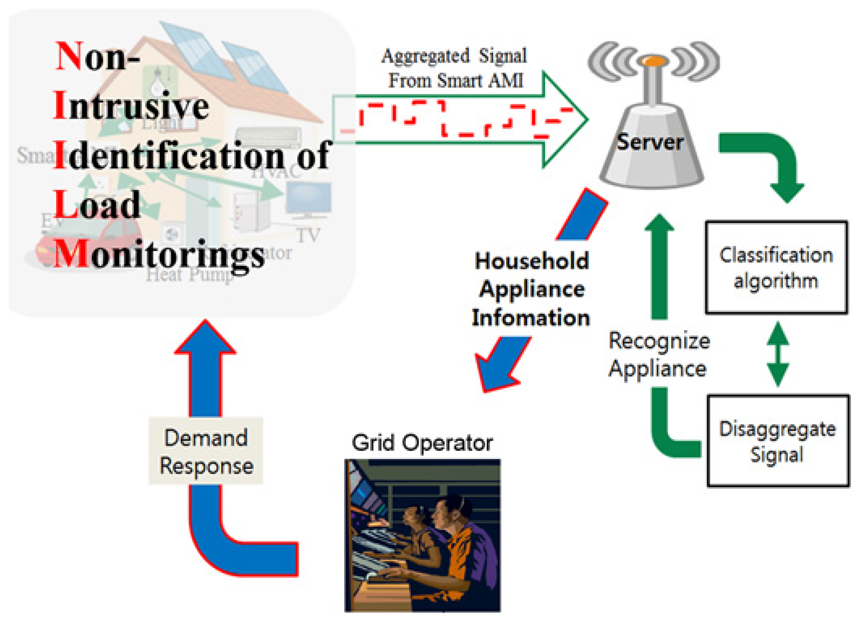
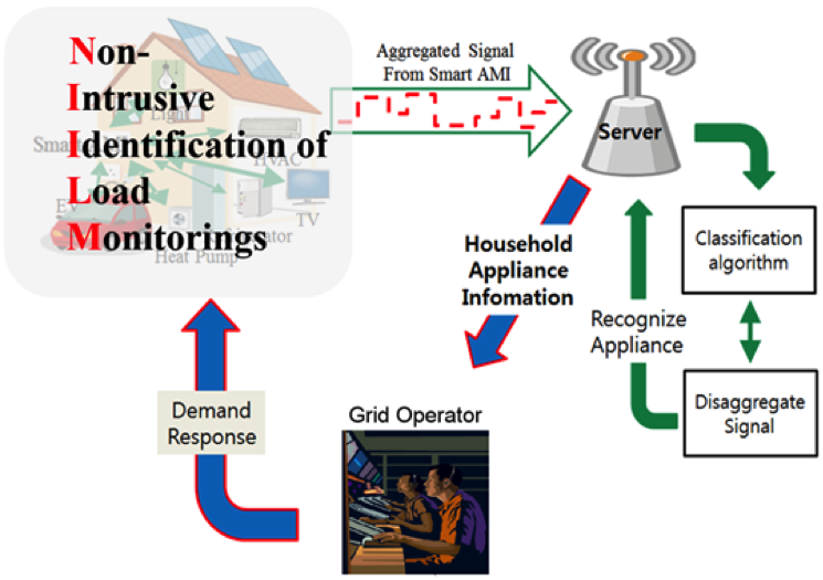
Figure 1.
System architecture.
Figure 1.
System architecture.
APD is the distribution of the usage of electronic appliances. The penetration rate is the average number of appliances per household in percentage. For example, a penetration rate of 90% for TV means that on average each household owns 0.9 TV (or 90% of households own one TV) and a penetration rate of 200% means that on average each household owns two TVs.
Table 1 shows some product cases with their penetration rate. The penetration rate of the appliance is used as feature to disaggregate aggregated load power.
Table 1.
Appliance penetration rate.
Table 1.
Appliance penetration rate.
| Product case | 2005 | 2010 | 2020 |
|---|
| Rate (%) | Rate (%) | Rate (%) |
|---|
| Mobile phone | 406 | 446 | 492 |
| Lighting | 93 | 107 | 143 |
| Radio | 60 | 60 | 60 |
| Electric toothbrush | 22.4 | 22.5 | 25.9 |
| Electric oven | 38 | 38 | 38 |
| TV+ | 144 | 202 | 210 |
| Washing machine | 96.6 | 97.9 | 100.0 |
| DVD | 75 | 90 | 130 |
| Audio mini system | 60 | 60 | 60 |
The usage pattern over a period of time can provide the frequency distribution of an appliance’s usage penetration. For instance, if at time t, the living room light is turn on over a period of time, T, the probability of the living room light being on at any time will be higher than the other appliances, which are rarely used.
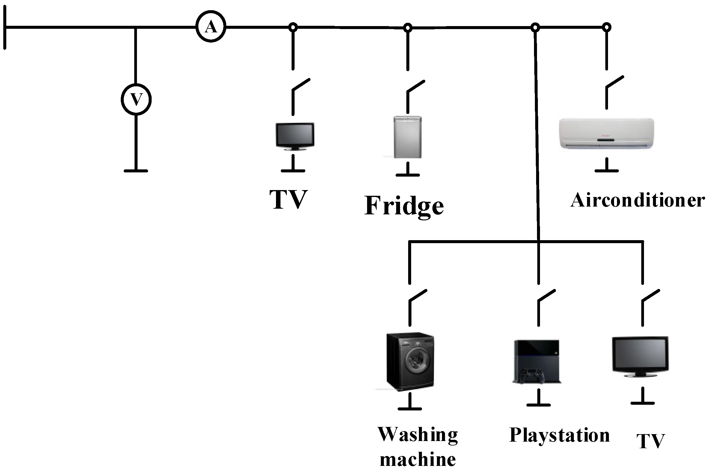
ADD describes the strong correlation in the usage pattern of some appliances with others. For instance, Playstation 4 cannot be used without a television and a stabilizer cannot be used without other appliances such as fridge, TV and audio system. We tested these dependencies with our dataset by measuring the correlation between every pair of appliances using Pearson’s coefficients. We subsequently computed the conditional probability of the appliance pairs that shows strong correlation. The conditional probabilities of the correlated pairs are used as a feature in disaggregating power.
3.4. Data Acquisition and Pre-Processing
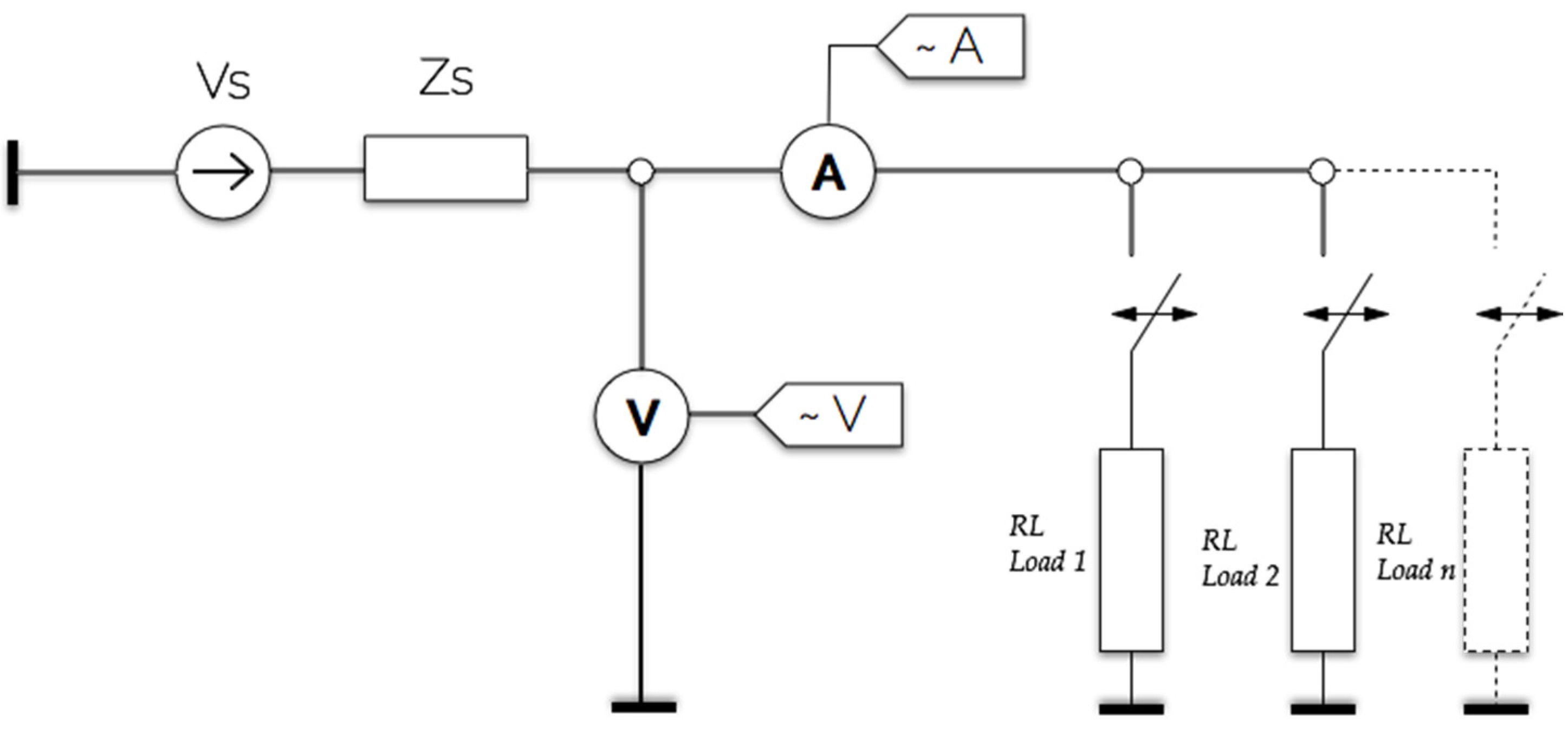
Figure 2 represents the power distribution layout of the household. In this simulated circuit, the voltage source supplying the household along with its internal impedance is designated as
Vs and
Zs respectively. The impedance reflects the voltage drop due to the loading of the electrical circuit.
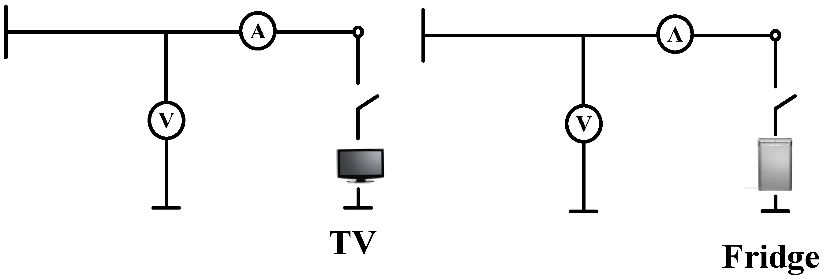
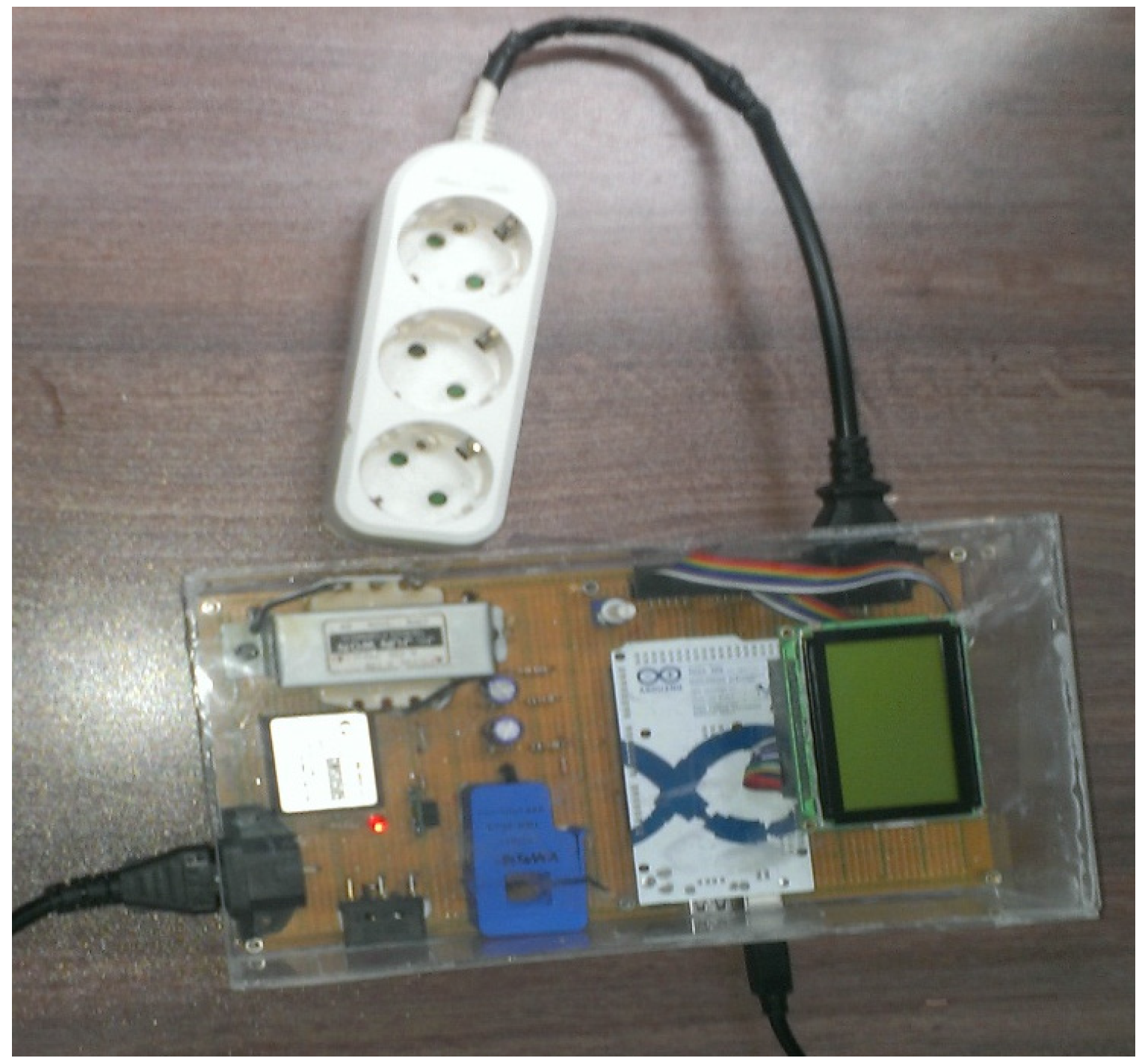
The measurement acquisition system includes an instantaneous current and voltage recorders together with the feature parameters. They are connected next to the voltage source in order to measure the total current of the household. The measured current and voltage instantaneous values are recorded and fed into the recognition algorithm. During this simulation, one appliance was connected at a time to measure its current and voltage within a specified time period. The measured parameters were stored in a database for processing. In a similar way, multiple appliances were connected at the same time and their parameters measured and stored.
Figure 2.
Single-phase power network.
Figure 2.
Single-phase power network.
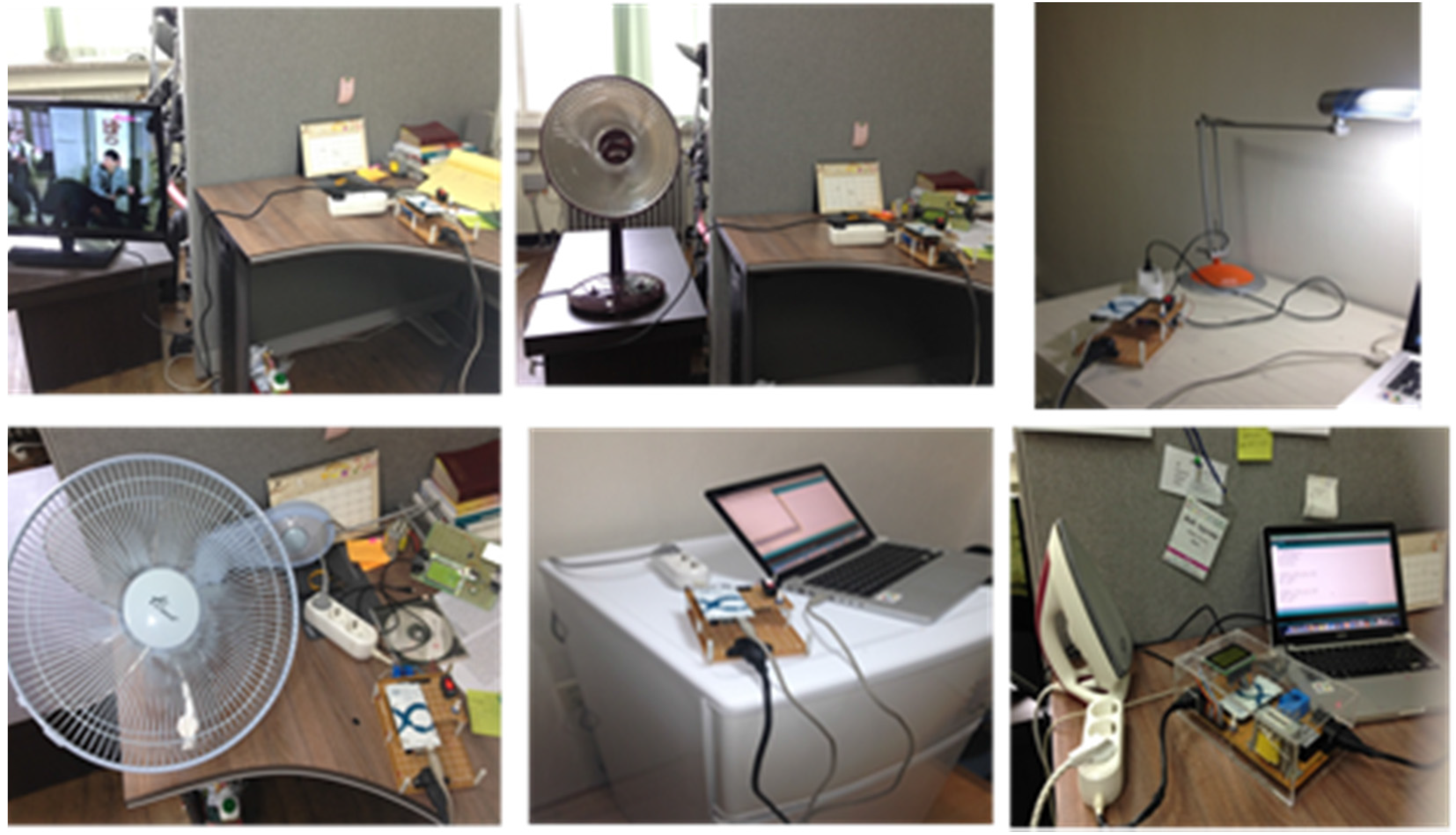
Six household electrical appliances were used as loads in this study: Fridge_new (Load 1), Fridge_old (Load 2), LCD_TV (Load 3), Desktop lamp (Load 4), Standing heater (Load 5) and wall fan (Load 6). These electrical appliances have the following operational states: two-state, multi-states and continuously variable state. Two measurement procedures were performed to collect data for each load.
Table 2 provides a detailed power rating of the listed appliances.
Table 2.
Appliance power ratings.
Table 2.
Appliance power ratings.
| No. | Appliance | I (A) | V (v) | P (W) | Frequency (Hz) |
|---|
| 1 | Fridge_new | 2.72 | 220 | 500 | 60 |
| 2 | Fridge_old | 2.72 | 220 | 500 | 60 |
| 3 | LCD TV | 0.27 | 220 | 60 | 60 |
| 4 | Desk lamp | 0.1 | 220 | 20 | 60 |
| 5 | Standing heater | 3.63 | 220 | 800 | 60 |
| 6 | Iron | 4.55 | 220 | 1000 | 60 |
The measured data were stored in a database for processing. The structure of the database was normalized to ensure data integrity and faster queries.
The measured data forms a pool of appliance signatures that could be represented by the matrix below:
For a given measured aggregated power
mv, the measured signal can be modeled a row vector:
where:
The initial step that was considered before finding the best combination that represents the data was to sort the appliance signatures. The sorting order of the signatures was based on the least value of the measured signal. After the data set has been sorted based on the sorting order, the data set was trimmed to eliminate records whose feature values are greater than the measured values. The new matrix has a record less than the original dataset.
3.5. Model Description
HMM is used for probabilistically modeling sequential data. HMMs are known to perform well at tasks such as speech recognition [
31]. A discrete-time HMM can be viewed as a Markov model whose states are not directly observed: instead, each state is characterized by a probability distribution function, modeling the observations corresponding to that state. Our model is based on HMM. We defined a probabilistic model that explains the generating process of the observed data. This model contains hidden variable that are not observed. With regards to our work, the states of the appliances are the hidden variables, and the aggregated features (
i.e.,
P,
Q,
H3,
H5,
H7) are the observations.
The model has several parameters that can be learned from the captured data. The learning process consists of estimating the factorial observations of the appliances. The parameters from the observation, such as the initial probability of selecting a given state and the transition probability and the observation probability estimate the model that best describe the observation. In order to achieve this, the parameters of the model are adjusted so as to maximize the efficiency of describing the model that best describe the observation. Subsequently, using this model with the estimated parameters, we can estimate the hidden variables, which are the states of the appliances. The pseudo-code for our algorithm is described below:
- (1)
Generate factorial states
- (2)
λ ← [A, B, π]; Initial parameters
- (3)
Repeat
- (4)
Q ← [q | λ]; Generate sequence
- (5)
λ′ ← λ; Generate new parameters
- (6)
Until λ converges
- (7)
q* ← ; The mostly like sequence
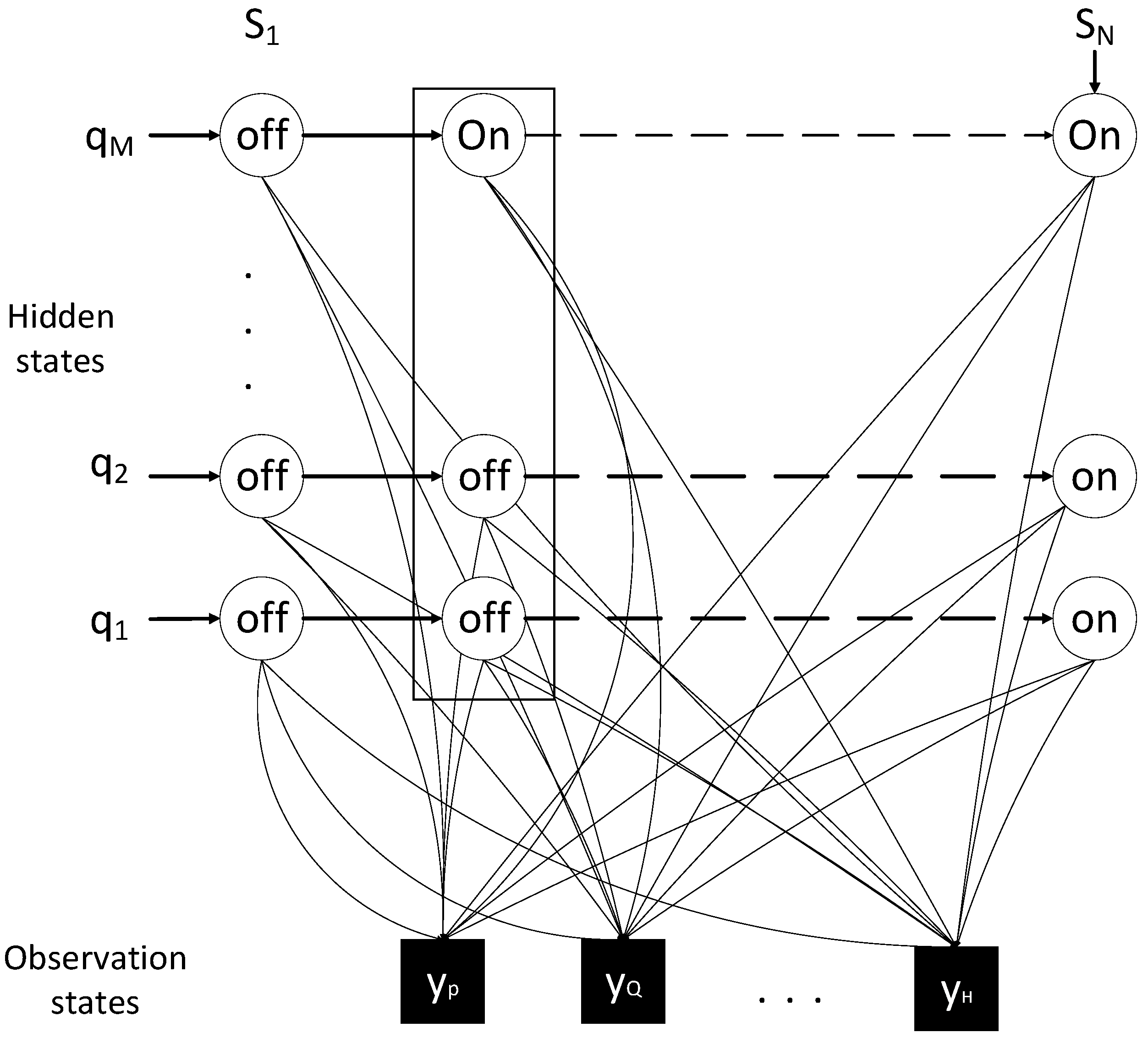
In
Figure 3, the network topology of MCFHMM where each of state consists of a list of appliances based on the factorial of the number of total appliances is shown. Each appliance has observation symbols, which contributes to the total measured observation symbols.
As stated in the earlier section, given the parameter estimator λ, where λ represent A, B, π and the Observation symbol, Y = {y1, y2, y3, …, yT}, How do we choose a corresponding state sequence Q = {q1, q2, q3, …., qM} which is optimal to the appliance state of operation and identification.
Mathematically, this quest can be express in the Equation (10):
Figure 3.
Network topology of multiple conditional factorial hidden Markov model (MCFHMM).
Figure 3.
Network topology of multiple conditional factorial hidden Markov model (MCFHMM).
For a single input,
Y will be constant and therefore so will
P(Y), so we only need to find:
: the probability of the observation sequence given the state sequence is the model likelihood, whereas
P(Q) the probability of the states is the prior probability of the sequence. It can be seen from the above algorithm that a complete specification of HMM requires specification of observation symbol, the specification of the state and the three probability measures A, B and π. For convenience, we use the compact notation:
The probability distribution for an appliance,
qi being ON can be defined as one minus the ratio of the error of the state to the total error of the model.
On the other hand, the probability distribution for an appliance,
qi being OFF can be defined as the ratio of the error of the state to the total error of the model:
The probability distribution for the observation,
can be defined as the observation over the total observations:
The initial state distribution,
= {
} where:
The Transition probability distribution, A = {
} is the movement from a state
to another state,
:
The observation symbol probability distribution in state j, B = {
} where:
i.e., the probability distribution is based on the dependency distribution between the appliances, the
APD and the observation distribution. Accordingly:
The
APD for a given state
j,
APD = {
Pj} where:
The
ADD = {
dij} for all the appliances in a given state j can be estimated by finding the Pearson correlation coefficient between each pair of appliances. The conditional probability of all the pair greater 0.9 is used as an additional feature,
i.e.,
The appliance usage penetration (AUP) =
for all the appliances in a given state
j, can be estimated as the sum of the probabilities of the occurrence of the appliances:
For a given set of parameter λ initially estimated, there is now the need to find how the choice of the sequence of the state has on the observation sequence, whether it could represent the given model. The joint probability of the observation sequence, Y and the set of the state sequence Q could be estimated by using the Forward-Backward procedure. Considering the forward variable, α
t(
i). We defined α
t(
i) as:
where
.
We estimated the probability of the partial observation sequence
y1,
y2, ···,
yt until time
t and the state
Si at time
t, given the model λ. What this means is that we solve α
t(
i) inductively. We initially estimated the forward variable by multiplying the initial observation symbol probability with its initial state distribution.
For N states, the initial forward variable generates a vector matrix, which consists of the probability of an appliance set,
occupying states
and the probability of its observation distribution. Subsequently, at time
t > 1, the forward variable could be estimated by induction as:
Similarly, we defined β
t(
i) as:
Finally, the joint probability of the observation sequence and the state sequence given a parameter could be defined as:
The main objective of the energy disaggregation algorithm is to discover the states of the appliances, which contribute to the observation sequence. Our focus is on the hidden states of the MCFHMM model that matches the observation sequence. After learning the parameter, λ, we estimated the most likely state sequence,
q* that maximize the model:


