
Increasing Fuel Efficiency of Direct Methanol Fuel Cell Systems with Feedforward Control of the Operating Concentration


Abstract
:
1. Introduction
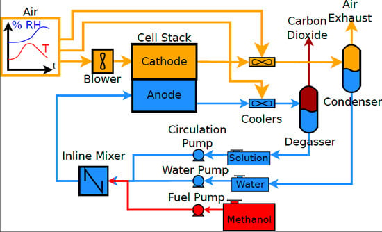
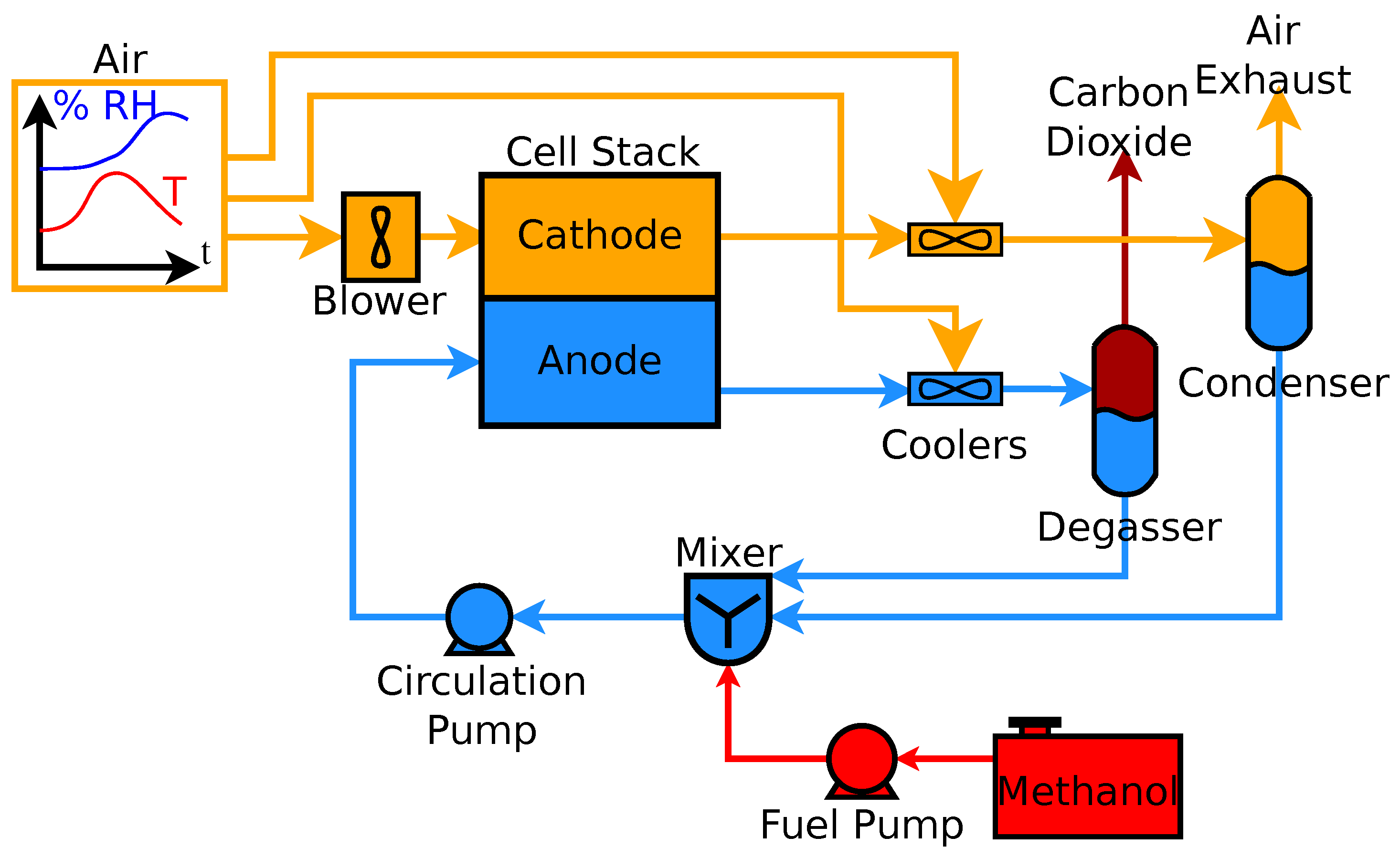
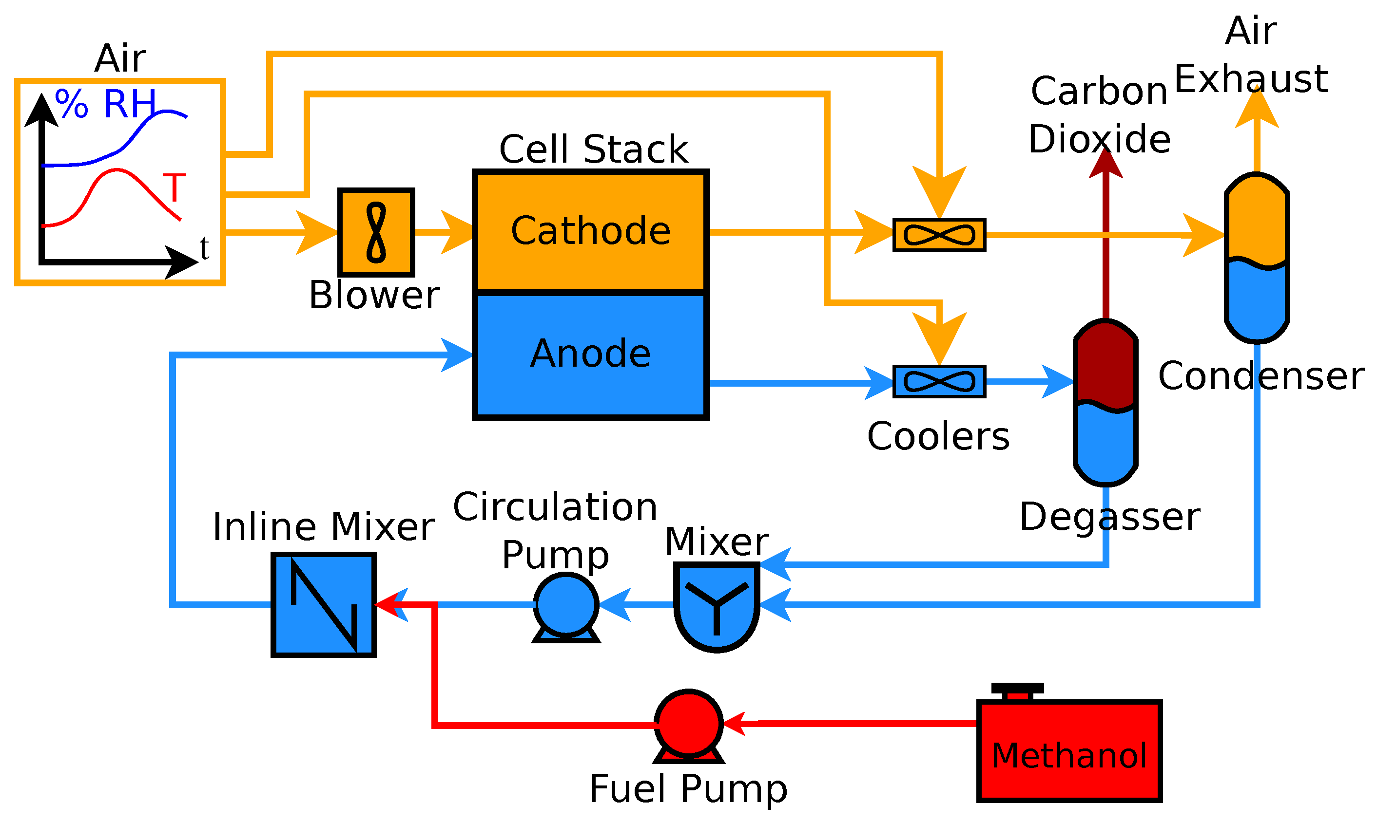
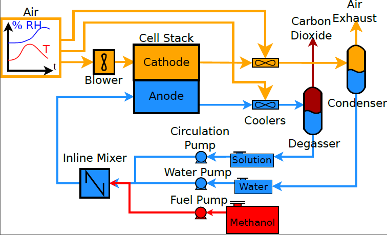
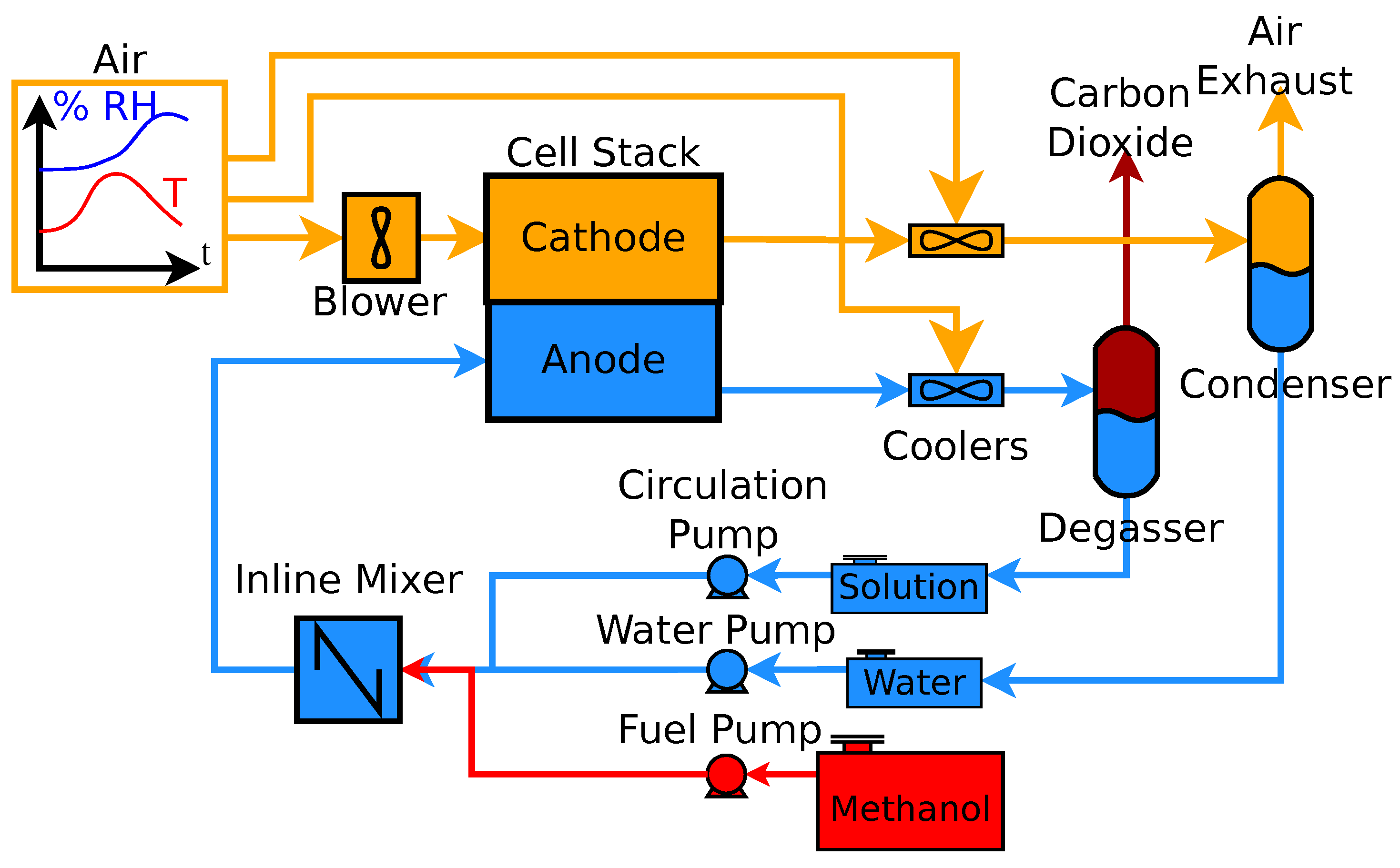
2. Systems

3. Methods
3.1. Modeling
3.1.1. Cell Model

| Components | Stack | |
|---|---|---|
| Component mass balance | (T1.1) | |
| Energy balance | (T1.2) | |
| Electro-osmotic water drag | (T1.3) | |
| Electro-osmotic drag coefficient | (T1.4) | |
| Index | ||
| Components | Separators | |
| Component mass balance | , | (T.15) |
| , | (T1.6) | |
| (T1.7) | ||
| Energy balance | (T1.8) | |
| Components | Mixer | |
| Component mass balance | (T1.9) | |
| Energy balance | (T1.10) |
3.1.2. Peripheral Devices
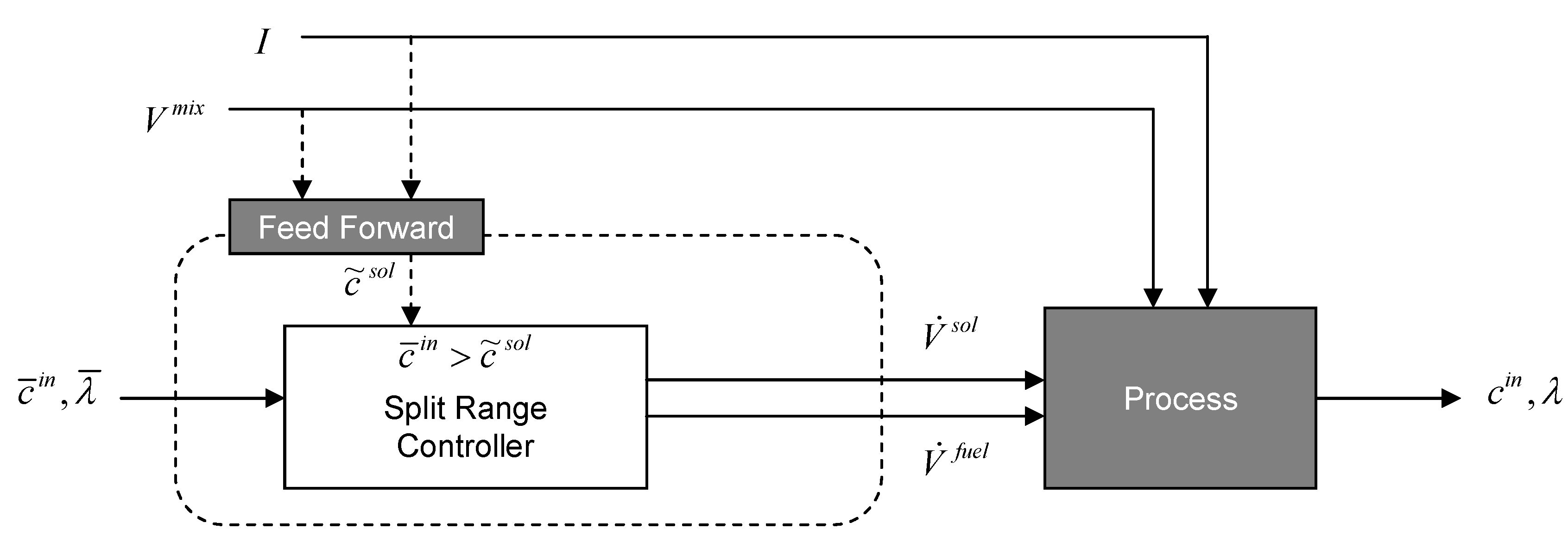
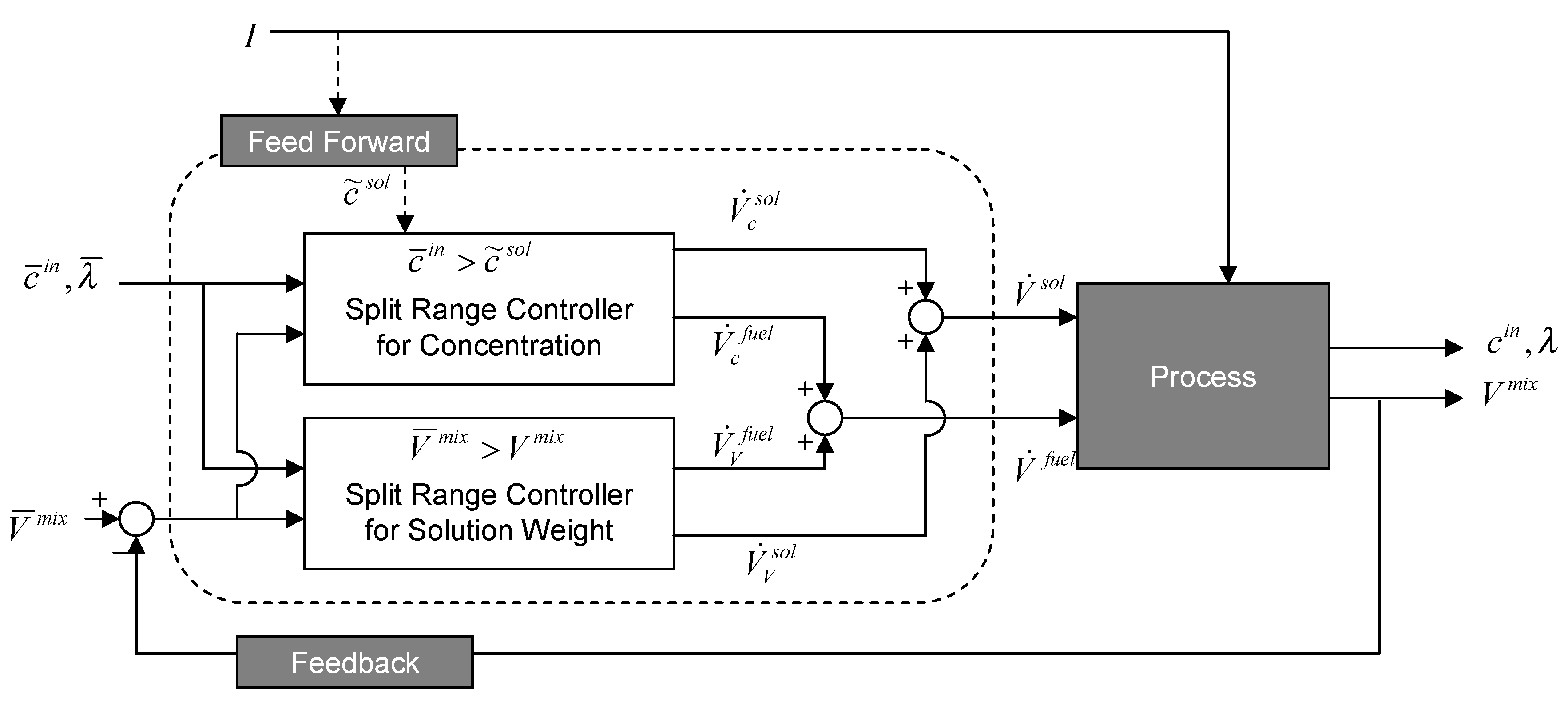
3.2. Controller Synthesis
| Controlled variable | Manipulated inputs | Disturbance | Measured outputs | Controller type |
|---|---|---|---|---|
| I, | I | Feedforward | ||
| I | I | Feedforward | ||
| I | I | Feedforward | ||
| Feedback | ||||
| I, | P feedback |
3.2.1. Concentration Set-Point
- Faradaic efficiency φ,
- Electrochemical efficiency ε and,
- Thermodynamic efficiency .
3.2.2. Concentration Estimate
3.2.3. Two-Mixer System

3.2.4. Separate Tank System
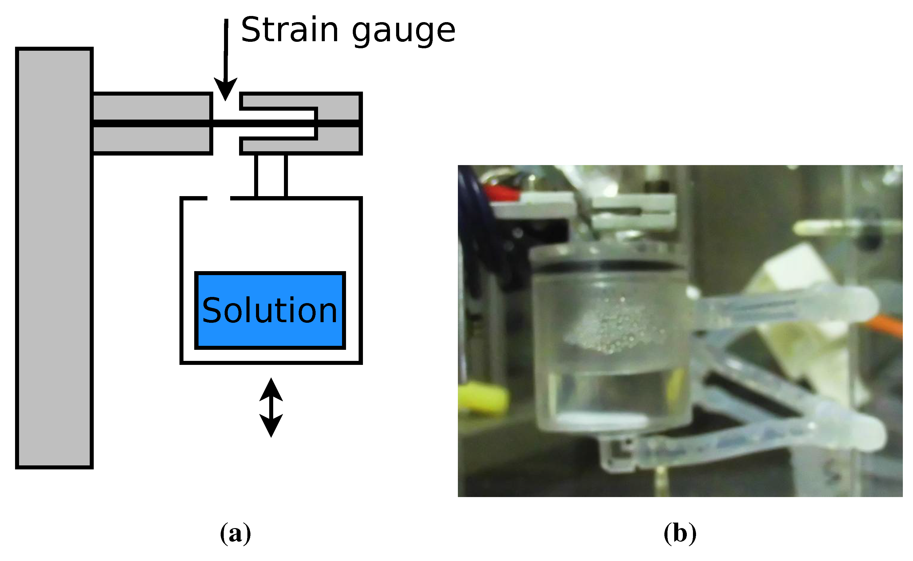
3.3. Experimental Setup
3.3.1. Equipment
3.3.2. Experimental Procedure
3.3.3. Error Analysis
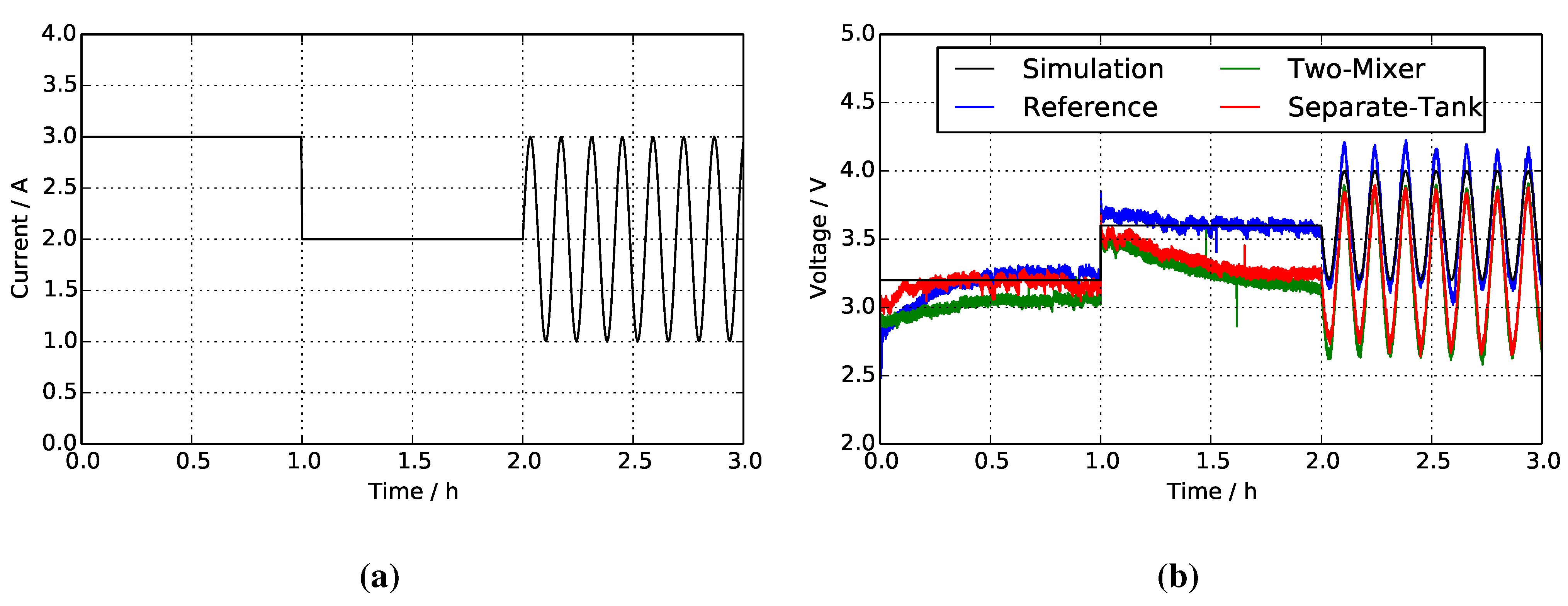
4. Results and Discussion

| Parameter | Reference | Two-mixer | Separate tanks |
|---|---|---|---|
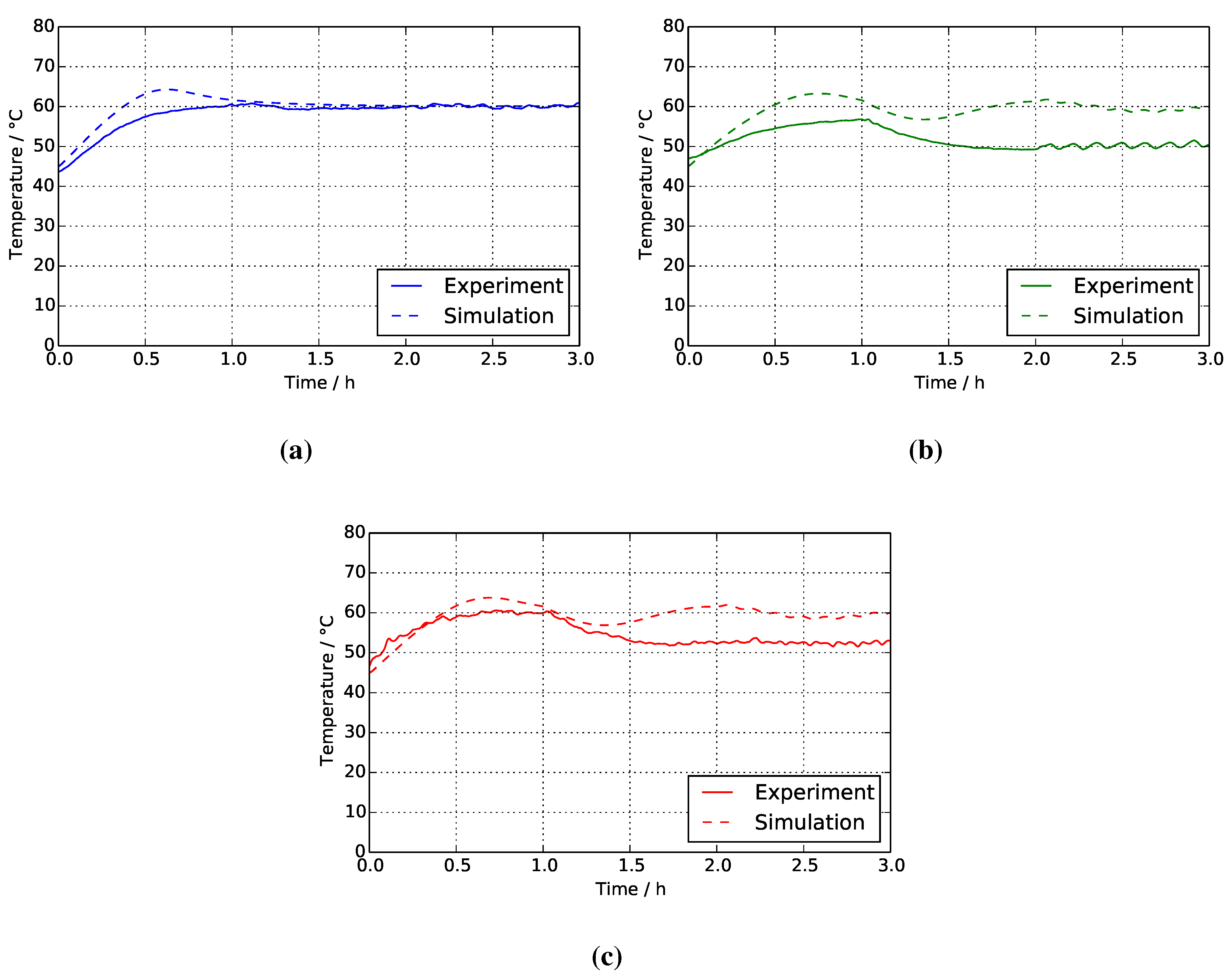
| Stack temperature /°C | 2.47 (Figure 8a) | 7.85 (Figure 8b) | 5.64 (Figure 8c) |
| Inlet concentration /M | 0.151 (Figure 9a) | 0.266 (Figure 9c) | 0.263 (Figure 9e) |
| Outlet concentration /M | 0.092 (Figure 9b) | 0.203 (Figure 9d) | 0.175 (Figure 9f) |
4.1. Reference System

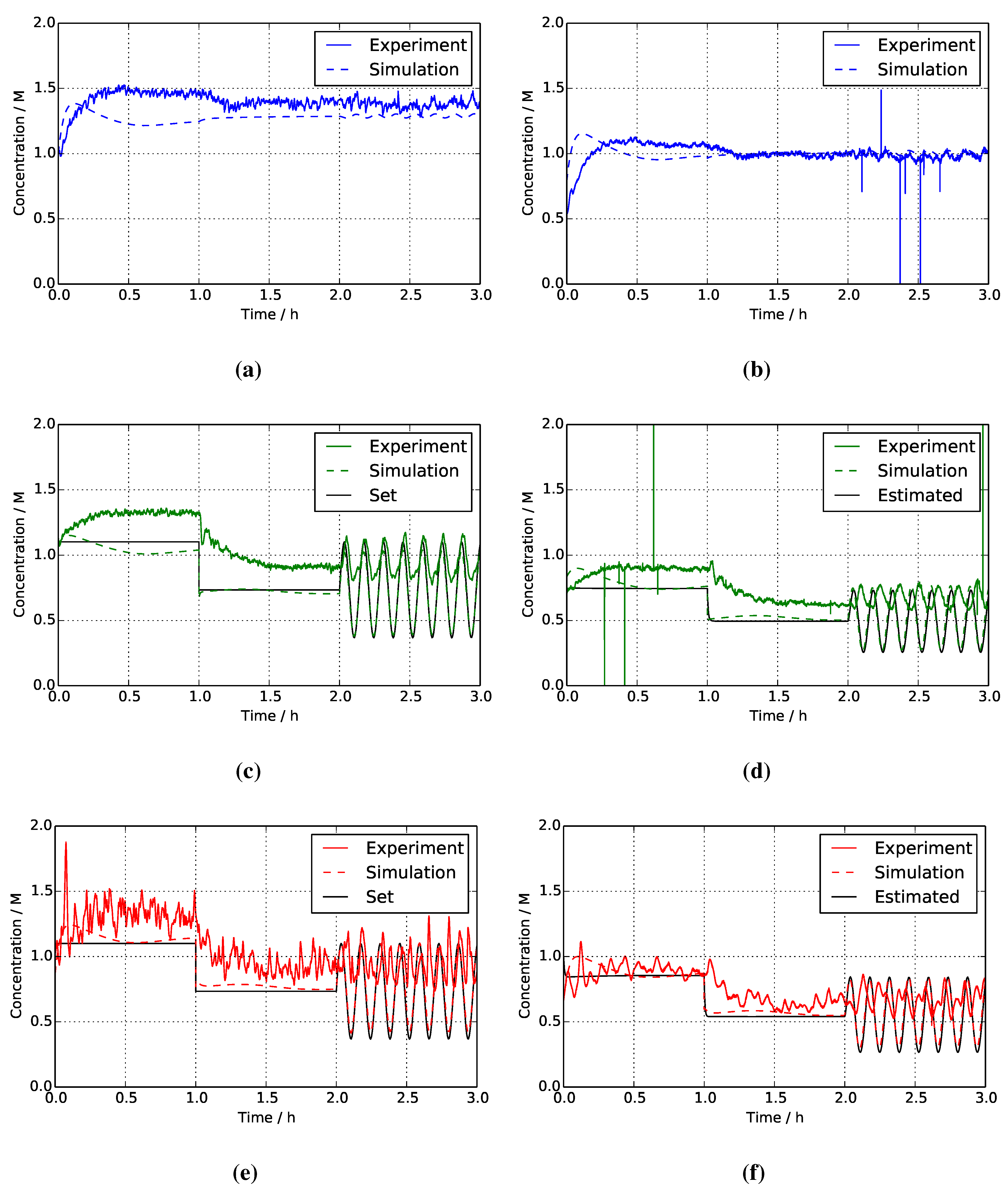
4.2. Two-Mixer System
4.3. Separate Tank System
4.4. Faradaic Efficiencies
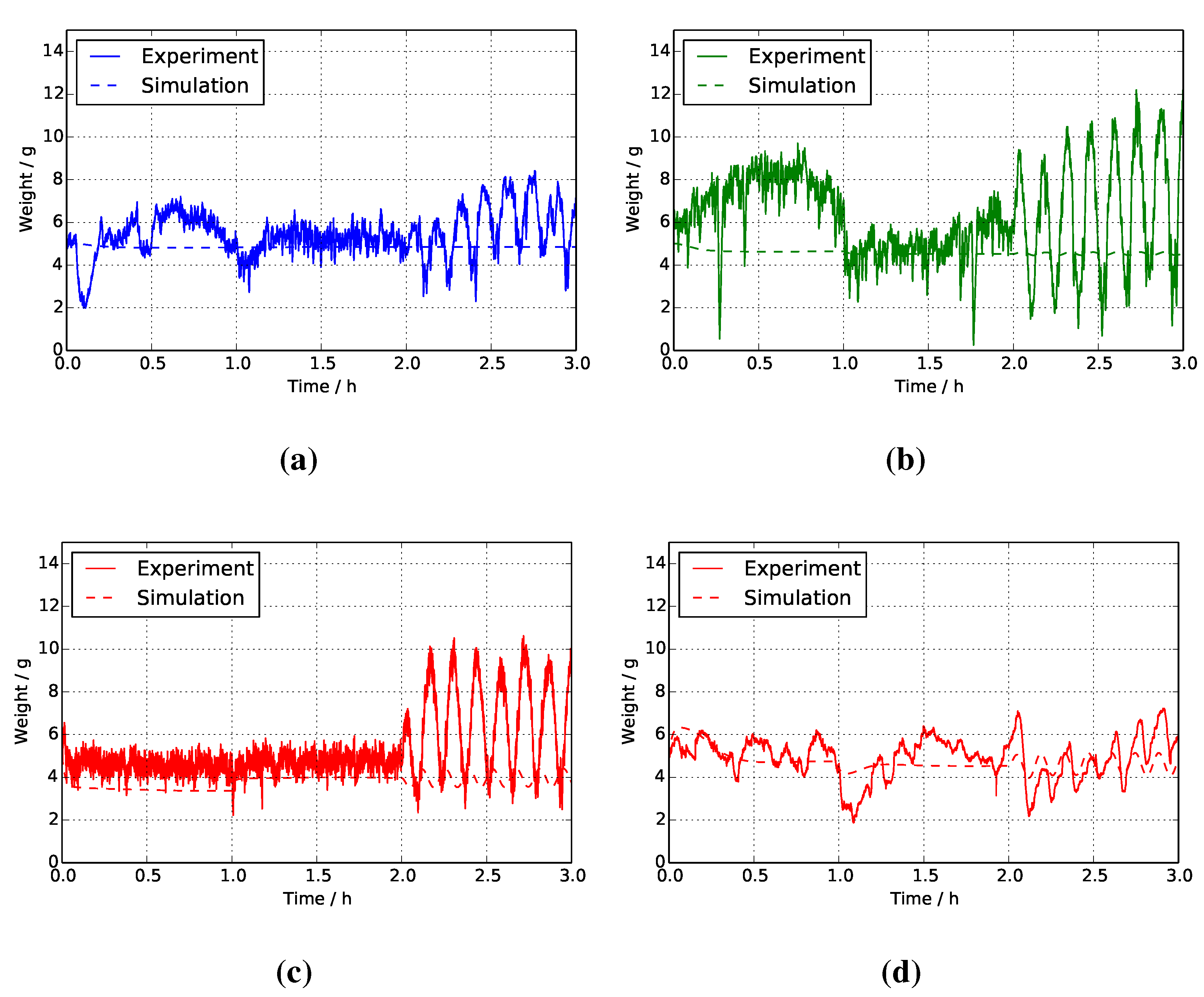
4.5. Liquid Holdup in Solution Tanks
5. Conclusions
Acknowledgments
Author Contributions
Conflicts of Interest
Latin Symbols
| a | Crossover parameter (= 1.6748 m/s) |
| A | Active area (= 0.003 m2) |
| b | Crossover parameter (= 0.173) |
| c | Concentration (mol/m) |
| E | Internal energy (J) |
Stack heat capacity (= 3000 J/K) | |
| i | Current density (A/cm2) |
| I | Current (A) |
| F | Faraday constant (= 96485 C/mol) |
Reaction Gibbs free energy (= −702 kJ/mol) | |
| h | Molar enthalpy (J/mol) |
Reaction enthalpy (= −726 kJ/mol) | |
Electro-osmotic drag coefficient (-) | |
| M | Molar mass (kg/mol) |
| N | Number of cells (= 9) |
| n | Amount of substance (mol) |
| R | Resistance (= 0.4 Ω) |
| U | Voltage (V) |
Open-circuit voltage (V) | |
| V | Volume (m3) |
| W | Weight (g) |
| y | Mole fraction (-) |
Greek Symbols
| β | Vapor molar fraction (-) |
| η | Overall efficiency (-) |
| φ | Faradaic efficiency (-) |
| ε | Electrochemical efficiency (-) |
| λ | Excess ratio (-) |
| ν | Current stoichiometric coefficient (-) |
| ξ | Crossover stoichiometric coefficient (-) |
| ρ | Density (kg/m3) |
| τ | Time constant (s) |
Superscripts
| an | Anode |
| cath | Cathode |
| cond | Condenser |
| deg | Degasser |
| fuel | Fuel |
| gas | Gas |
| ater | Water |
| liq | Liquid |
| mix | Mixer or solution tank |
| s | Side of anode or cathode |
| sol | Solution |
| stack | Stack |
Subscripts
| flows | Flows to the mixer from condenser, degasser or fuel reservoir |
| in | Inlet |
| j | Species |
| out | Outlet |
| x | Crossover |
Diacritics
estimate | |
set point | |
flow (s−1) |
References
- Carter, D.; Ryan, M.; Wing, J. The Fuel Cell Industry Review 2012; Technical Report for Fuel Cell Today: Hertfordshire, UK, 2012. [Google Scholar]
- Sharaf, O.Z.; Orhan, M.F. An overview of fuel cell technology: Fundamentals and applications. Renew. Sustain. Energy Rev. 2014, 32, 810–853. [Google Scholar] [CrossRef]
- Kamarudin, S.K.; Daud, W.R.W.; Ho, S.L.; Hasran, U.A. Overview on the challenges and developments of micro-direct methanol fuel cells (DMFC). J. Power Sources 2007, 163, 743–754. [Google Scholar] [CrossRef]
- Kim, J.H.; Yang, M.J.; Park, J.Y. Improvement on performance and efficiency of direct methanol fuel cells using hydrocarbon-based membrane electrode assembly. Appl. Energy 2014, 115, 95–102. [Google Scholar] [CrossRef]
- Tsai, M.C.; Yeh, T.K.; Chen, C.Y.; Tsai, C.H. A catalytic gas diffusion layer for improving the efficiency of a direct methanol fuel cell. Electrochem. Commun. 2007, 9, 2299–2303. [Google Scholar] [CrossRef]
- Meyers, J.P.; Bennett, B. Analytical model to relate DMFC material properties to optimum fuel efficiency and system size. J. Power Sources 2011, 196, 9473–9480. [Google Scholar] [CrossRef]
- Park, J.Y.; Seo, Y.; Kang, S.; You, D.; Cho, H.; Na, Y. Operational characteristics of the direct methanol fuel cell stack on fuel and energy efficiency with performance and stability. Int. J. Hydrog. Energy 2012, 37, 5946–5957. [Google Scholar] [CrossRef]
- Wu, W.; Lin, Y. Fuzzy-based multi-objective optimization of DMFC system efficiencies. Int. J. Hydrog. Energy 2010, 35, 9701–9708. [Google Scholar] [CrossRef]
- Arisetty, S.; Jacob, C.A.; Prasad, A.K.; Advani, S.G. Regulating methanol feed concentration in direct methanol fuel cells using feedback from voltage measurements. J. Power Sources 2009, 187, 415–421. [Google Scholar] [CrossRef]
- Zenith, F.; Krewer, U. Modeling, dynamics and control of a portable DMFC system. J. Process Control 2010, 20, 630–642. [Google Scholar] [CrossRef]
- Zenith, F.; Krewer, U. Simple and reliable model for estimation of methanol cross-over in direct methanol fuel cells and its application on methanol-concentration control. Energy Environ. Sci. 2011, 4, 519–527. [Google Scholar] [CrossRef]
- Zhao, T.; Xu, C.; Chen, R.; Yang, W. Mass transport phenomena in direct methanol fuel cells. Progress Energy Combust. Sci. 2009, 35, 275–292. [Google Scholar] [CrossRef]
- Scott, K.; Taama, W.; Kramer, S.; Argyropoulos, P.; Sundmacher, K. Limiting current behaviour of the direct methanol fuel cell. Electrochim. Acta 1999, 45, 945–957. [Google Scholar] [CrossRef]
- Zenith, F.; Na, Y.; Krewer, U. Effects of process integration in an active direct methanol fuel-cell system. Chem. Eng. Process. Process Intensif. 2012, 59, 43–51. [Google Scholar] [CrossRef]
- Skogestad, S. Simple analytic rules for model reduction and PID controller tuning. J. Process Control 2003, 13, 291–309. [Google Scholar] [CrossRef]
© 2015 by the authors; licensee MDPI, Basel, Switzerland. This article is an open access article distributed under the terms and conditions of the Creative Commons Attribution license (http://creativecommons.org/licenses/by/4.0/).
Share and Cite
Na, Y.; Zenith, F.; Krewer, U. Increasing Fuel Efficiency of Direct Methanol Fuel Cell Systems with Feedforward Control of the Operating Concentration. Energies 2015, 8, 10409-10429. https://doi.org/10.3390/en80910409
Na Y, Zenith F, Krewer U. Increasing Fuel Efficiency of Direct Methanol Fuel Cell Systems with Feedforward Control of the Operating Concentration. Energies. 2015; 8(9):10409-10429. https://doi.org/10.3390/en80910409
Chicago/Turabian StyleNa, Youngseung, Federico Zenith, and Ulrike Krewer. 2015. "Increasing Fuel Efficiency of Direct Methanol Fuel Cell Systems with Feedforward Control of the Operating Concentration" Energies 8, no. 9: 10409-10429. https://doi.org/10.3390/en80910409