1. Introduction
A practical gearbox system for wind turbines or vehicle manual transmissions under excitation conditions shows severe vibro-impacts due to clearance-type nonlinearities [
1,
2,
3,
4,
5,
6,
7,
8,
9]. In general, clearance-type nonlinearties mean the nonlinear characteristics caused by the clearance such as a distance between two sub-systems. For example, a gear backlash is a representative clearance located between two gear teeth where repetitive separation and contact motions are caused by various engine input conditions, which produce severe vibro-impacts due to the alternating engine input torque flow. Regarding these vibro-impacts, various methods have been suggested to understand the impact phenomena caused by clearances such as gear backlash. For example, Padmanabhan and Singh [
1] employed the harmonic balance method (HBM) to simulate neutral gear rattle in an automotive transmission. Kim
et al. [
3] examined impact damping with clearance-type nonlinearities with focus on gear backlash. Yoon and Lee [
8] used two smoothening factors to investigate practical nonlinear dynamic behaviors due to piecewise-type nonlinearities. Yoon and Yoon [
9] employed the HBM to investigate the dynamic characteristics of a single-degree-of-freedom (DOF) torsional system accompanied by a multi-stage clutch damper model. Other studies have examined various vibration problems using the HBM [
10,
11,
12,
13,
14,
15,
16,
17,
18,
19,
20,
21,
22]. For instance, nonlinear problems using a Duffing oscillator or cubic stiffness have been settled by utilizing the nonlinear output frequency response functions (NOFRFs) and incremental harmonic balance (IHB) method [
10,
11]. Also, chaotic behaviors of physical systems have been examined [
12,
13]. Additionally, the response of a system with a hysteretic restoring force has been studied by applying two degree of freedom chain systems with sinusoidal inputs [
14]. Incremental or multi-component HBMs have been employed as well to investigate the nonlinear system responses [
15,
16,
17,
18]. The time domain responses for the
ith sub-system have been extended based upon the Galerkin scheme [
19,
20,
21,
22]. Although many studies have investigated clearance-type nonlinearities, difficulties still remain in implementing these methods on practical systems.
As an example of geared systems, a manual transmission driveline is introduced for this research and the dynamic behaviors of such systems can be generally observed in other geared systems such as wind turbines. As the theoretical background of this study contains the concepts of gear contact/separation as well as transmission errors describing the relationship of gear mesh forces
vs. relative displacement of the gear pair, the scope of this research can be adapted to macro scale geared system such as wind turbine system drivelines.
Figure 1 shows a reduced-order model of a manual transmission driveline, which is an example of a physical system, with pertinent nonlinear elements [
7,
8]. It is a 5-speed manual transmission model with parallel type gears. The transmission is assumed to be under the third gear engaged and the fifth gear unloaded status. The order of the original system has been reduced so that most of the speed gears are unloaded and rotating except for one engaged through the synchronizer and gear-shifting mechanism. The key components such as the gear pairs, the clutch hub, the flywheel, the input shaft, the axles and the tire-vehicle system are characterized by the lumped torsional inertia
I or stiffness
k. The fixed gears and the synchronizer assembly are considered as the input and output shafts. The reduced model with six DOF is the minimum level of system that can accommodate all the key parameters, such as the multi-stage clutch dampers, drag torques, and gear backlash on both engaged and unloaded gear pairs. These nonlinearities are illustrated in the schematic diagram shown in
Figure 1. Definitions of the key parameters are listed in
Table 1.
Figure 1.
A nonlinear torsional system model with six degrees of freedom with multiple nonlinearites.
Figure 1.
A nonlinear torsional system model with six degrees of freedom with multiple nonlinearites.
Table 1.
Definitions of key parameters.
Table 1.
Definitions of key parameters.
| Key parameters | Definition | Key parameters | Definition |
|---|
| Fgu | Gear mesh force of unloaded gear | θh | Absolute motion of clutch hub |
| Fge | Gear mesh force of engaged gear | θi | Absolute motion of input shaft |
| TE | Input (engine) torque | θou | Absolute motion of unloaded gear |
| TC | Overall clutch torque | θo | Absolute motion of output shaft |
| TDi | Drag torque on input shaft | θv | Absolute motion of vehicle |
| TDo | Drag torque on output shaft | ch | Damping of clutch hub |
| TDu | Drag torque on unloaded gear | ci | Damping of input shaft |
| TDVE2 | Drag torque on vehicle | cg | Damping of gear mesh |
| If | Inertia of flywheel | cVE2 | Damping of vehicle |
| Ih | Inertia of clutch hub | ki | Stiffness of input shaft |
| Iie | Inertia of input shaft | kVE2 | Stiffness of vehicle |
| Iou | Inertia of unloaded gear | Riu | Radius of unloaded gear on input shaft |
| IOG | Inertia of output shaft | Rie | Radius of engaged gear on input shaft |
| IVE2 | Inertia of vehicle | Rou | Radius of unloaded gear on output shaft |
| θf | Absolute motion of flywheel | Roe | Radius of engaged gear on output shaft |
Figure 2 illustrates the piecewise-type nonlinearity between the flywheel and clutch hub and clearance-type nonlinearity between engaged and unloaded gear pairs [
7,
8,
9]. In this figure, clutch torque profiles are expressed including hysteresis levels and transition angles. A nonlinear function
TC has been depicted by the relationship of clutch torque
vs. relative displacement
δ1Pr. This profile is measured under the static load conditions when the torque levels of multi-staged linear torsional spring are determined by both
δ1Pr and
, which is defined as the relative velocity between clutch and flywheel.
TC,
δ1pr, and
kCn indicate overall clutch torque, relative displacement between the flywheel and the clutch hub, and torsional stiffness of
nth stage clutch damper, respectively.
Figure 2b indicates the expected gear mesh force with the relationship of the relative displacement of the gear pair
δ vs. the gear mesh force
F. Here,
kg and
b indicate the gear mesh stiffness and the gear backlash, respectively. Observing this figure, the dynamic conditions of the forces are abruptly changed at
b/2 or −
b/2. To simulate strong nonlinearities at multiple points in the torsional system, the HBM will be used by extending the previously proposed basic formulations [
9,
22]. In addition, this study examines the nonlinear behaviors of an impact pair from the geared systems, in the frequency domain, by extending prior impact pair analysis [
23].
Figure 2.
Nonlinear characteristics of multi-stage clutch dampers and gear backlash: (a) Nonlinear function
for multi-stage clutch dampers; (b) Gear mesh force.
Figure 2.
Nonlinear characteristics of multi-stage clutch dampers and gear backlash: (a) Nonlinear function
for multi-stage clutch dampers; (b) Gear mesh force.
The specific objectives of this study are as follows: (1) the dynamic behaviors of impact pairs in a geared system were investigated by implementing piecewise-type nonlinearities at multiple points; (2) the effects of key parameters on the vibro-impacts were examined using the HBM to improve the vibratory conditions; and (3) the impact phenomena were numerically mapped in the bifurcation diagrams for the key parameters, which provides insight into the gear rattle criteria. Overall, within the scope described above, this research could help readers understand the basic concepts of the geared systems so that they can develop specific simulation methods of highly nonlinear systems such as wind turbines.
2. Problem Formulation with 6-DOF Nonlinear System Model
Based on the nonlinear system shown in
Figure 1, the basic equations are derived as follows [
7,
8,
9]. A reduced 6-DOF torsional system model is considered in this research, since a larger dimension may cause problems for nonlinear analysis. It includes nonlinear terms describing the clutch torque
TC, unloaded gear force
Fgu, and engaged gear force
Fge. The governing equations are derived from the moment equilibrium of each segment and placed in the matrix form. Assuming that drag torques are constant, the governing equations are given as:
Here,
θk(
t) (
k =
f,
h,
i,
ou,
o,
v) is the absolute motions of sub-systems such as the flywheel, clutch hub, input shaft, unloaded gear, output shaft, and vehicle. Equations (1a)–(1f) can be expressed in the matrix formulation by defining a state vector
as follows.
Here,
M,
C, and
K are inertia, damping, and stiffness matrices, respectively, and
and
are a nonlinear function and input torque vectors respectively. The other parameter designations and the values used in the simulation are summarized in
Table 2 and
Table 3 [
7,
8,
9,
22]. The employed nonlinear models can be derived as follows [
7,
8]. The nonlinear function describing the overall clutch torque
TC is defined as the summation of the preload torque
TSPr, stiffness torque
TS, and hysteresis torque
TH:
The torque caused by the preload
TSPr is determined by the function of relative displacement
δ1pr:
Here,
TPr1 and
TPr2 indicate the positive and negative preload,
σC is a smoothening factor, and
φPr is the phase at the preload when
δ1 is zero, respectively. The clutch torque resulted by the stiffness
TS(
δ1) is defined as follows:
In these equations,
kC(
i) is the clutch stiffness,
Dsp(
i) and
Dsn(
i) are the positive and negative sides of the clutch displacements induced by stiffness at the
ith stage, and
φp(
i) and −
φn(
i) are the
ith transition angles of the positive and negative sides. The torque due to hysteresis
TH for the multi-staged clutch under asymmetric transition angles is determined as follows:
where
H(
i) indicates the
ith stage of hysteresis and
DHp(
i) and
DHn(
i) stand for the positive and negative sides of relative motions resulted by hysteresis at the
ith stage, respectively.
Table 2.
Employed values of the torsional system parameters [
7,
8].
Table 2.
Employed values of the torsional system parameters [7,8].
| Inertia | Value (kg·m2) | Stiffness | Value (Nm·rad−1) | Radius | Value (mm) |
|---|
If
(Flywheel) | 1.38 × 10⁻¹ | kC
(Clutch for the linear model) | 1838.0 | Rie
(Engaged gear on the input shaft) | 35.5 |
Ih
(Clutch hub) | 5.76 × 10⁻³ | ki
(Input shaft) | 10000 | Roe
(Engaged gear on the output shaft) | 46.0 |
Iie
(Input shaft) | 4.53 × 10⁻³ | kVE2
(Drive shaft) | 6.63 × 10² | Riu
(Unloaded gear on the input shaft) | 45.9 |
IOG
(Output shaft) | 7.80 × 10⁻³ | kg
(Gear mesh) | 2.7 × 10⁸ (Nm−1) | Rou
(Unloaded gear on the output shaft) | 35.6 |
Iou
(Unloaded gear) | 5.23 × 10⁻⁴ | | | | |
IVE2
(Vehicle) | 3.27 | | | | |
The nonlinear function for the gear mesh force
Fg is defined as the following equation.
Here, b is defined as the gear backlash and the subscripts e and u are “engaged’ and ‘unloaded”. σg is the smoothening factor in the calculation of the gear mesh force.
In Equations (3)–(7b), the nonlinear function for the overall clutch torque
TC is the summation of the pre-load torque
TSPr, stiffness torque
TS, and hysteresis torque
TH. All of the clutch torques are expressed as a function of relative displacement
δ1pr given by Equation (4b), where
is the phase at the pre-load when the relative motion
δ1 between the flywheel and clutch hub is zero [
7,
8,
9].
TPr1 and
TPr2 are the positive and negative pre-loads, and
,
, and
are smoothening factors for the clutch stiffness, hysteresis, and gear backlash, respectively. Values of 1 × 10
2, 0.1, and 1 × 10
10 are employed for
,
, and
to calculate the clutch torques induced by the stiffness, hysteresis, and gear mesh forces, respectively [
7,
8,
9]. These smoothening factors are used for numerical convergence, especially for the stiff problem, and they are determined to minimize the difference between the physical discontinuities and smoothened simulation functions [
7,
8,
9].
Table 3.
Property values of the real-life multi-stage clutch damper [
7,
8].
Table 3.
Property values of the real-life multi-stage clutch damper [7,8].
| Property | Stage | Value |
|---|
Torsional stiffness, kCi
(linearized in a piecewise manner)
(Nm/rad) | 1 | 10.1 |
| 2 | 61.8 |
| 3 | 595.8 |
| 4 | 1838.0 |
| Hysteresis, Hi (Nm) | 1 | 0.98 |
| 2 | 1.96 |
| 3 | 19.6 |
| 4 | 26.5 |
Transition angle at positive side
(δi > 0), (rad) | 1 | 0.05 |
| 2 | 0.16 |
| 3 | 0.30 |
| 4 | 0.39 |
Transition angle at negative side
(δi < 0), (rad) | 1 | −0.04 |
| 2 | −0.05 |
| 3 | −0.09 |
| 4 | −0.15 |
kC(i) is the clutch stiffness,
Dsp(i) and
Dsn(i) are the switching functions at positive and negative sides of clutch relative velocities at the
ith stage [
9], and
and
are the
ith transition angles of the positive and negative sides, respectively.
H(i) is the
ith stage of hysteresis, and
DHp(i) and
DHn(i) are the positive and negative sides of the relative motions induced by hysteresis at the
ith stage, respectively. The nonlinear function for the gear mesh force
Fg is expressed by the gear backlash
b, and subscripts
e and
u indicate engaged and unloaded states. The transitional relative displacements between gear pairs are denominated by
ρe and
ρu. The properties employed for the multi-stage clutch damper are summarized in
Table 3. A value of 0.1 mm is given for
b [
7,
8].
To determine the dynamic characteristics in terms of natural frequencies and mode shapes based on the linear time-invariant (LTI) assumption, a clutch stiffness value of
kC = 1838.0 Nm∙rad
−1 is employed in Equation (5a) from
Table 3, since the 4
th stage of torsional spring is operating under the given excitation condition. The natural frequencies based on the eigensolutions are
f1 = 7.5 Hz,
f2 = 60.6 Hz, and
f3 = 273 Hz [
7,
8]. To focus on impact phenomena such as gear rattle, the main resonance regime centers on
f2 = 60.6 Hz, because the physical driveline with a 4-cylinder engine is normally excited by gear impacts between 700 RPM (23.3 Hz) and 3000 RPM (100 Hz) [
7,
8]. Thus, the frequency will be normalized with
f2 = 60.6 Hz in further calculations. The driveline shown in
Figure 1 is assumed to be in steady state given the sinusoidal excitations.
3. HBM and Numerical Simulation (NS) with Jumping Phenomena
By employing the HBM from prior studies [
9,
22], the nonlinear system responses with multiple locations of nonlinearities such as multi-stage clutch damper and gear backlash can be simulated based on the Galerkin scheme.
Figure 3 shows a comparison of the HBM and numerical simulation (NS) results with focus on the maximum, mean, and minimum values in the time history of the relative displacement of the unloaded gear pair
δ4(t), which can be calculated with the following equation. In this simulation, the normalized frequency
is used:
To simulate the time responses using NS, the modified Runge-Kutta method has been employed [
7,
8]. Since the gear impact phenomenon consists of many super-harmonics, the simulation becomes more reliable as the number of harmonics
Nmax is increased [
8]. However, this study is mainly limited to
Nmax ≤ 6 due to calculation time and convergence problems, which occur when the number of harmonics is increased beyond 6, such as
Nmax = 8 or 12. Here,
η indicates the sub-harmonic index.
The input torque
TE(
t) with
Nmax is calculated using the mean value of the input torque
Tm and the alternating part of the engine torque
Tpi as follows:
In this equation,
ωp and
are the firing frequency and phase, respectively. Directly measured values from an engine dynamometer test of
Tm = 168.9 Nm,
Tpi = 251.5 Nm, and
rad are employed for the HBM analysis [
7,
8].
Figure 3.
Comparison of the HBM (
Nmax = 6 and
η = 2) results with the NS results in the frequency domain. Key: ───, HBM;
![Energies 08 08924 i001]()
, NS by frequency up-sweeping;
![Energies 08 08924 i002]()
, NS by frequency down-sweeping.
Figure 3.
Comparison of the HBM (
Nmax = 6 and
η = 2) results with the NS results in the frequency domain. Key: ───, HBM;
![Energies 08 08924 i001]()
, NS by frequency up-sweeping;
![Energies 08 08924 i002]()
, NS by frequency down-sweeping.
To estimate the dynamic behaviors of the impact pair, the damping matrix is constructed using the assumed modal damping ratio
ζ = 0.02, since it is much difficult to physically measure [
7]. In addition, drag torques of Case IV in
Table 4 are used for the baseline for this study since there is no impact with Case IV which will be explained more in detail. The drag torque values are given by assuming 4 different cases: Case I, vehicle normal driving condition; Case II, severe dynamic conditions of gearbox system; Case III, severe gear impact condition; Case IV, the most stable condition.
Table 4.
Employed properties for the drag torques for various conditions [
7,
8].
Table 4.
Employed properties for the drag torques for various conditions [7,8].
| Drag torque (Nm) | Value |
|---|
| Case I | Case II | Case III | Case IV |
|---|
| Drag torque on the input shaft, TDi | 75.0 | 11.9 | 48.4 | 30.8 |
| Drag torque on the output shaft, TDo | 57.9 | 9.2 | 37.4 | 23.8 |
| Drag torque on the unloaded gear, TDu | 3.9 | 3.1 | 2.5 | 7.2 |
| Drag torque on the vehicle, TDVE2 | 57.3 | 189.0 | 114.6 | 143.2 |
As shown in
Figure 3, the HBM and NS results in the frequency domain match well with each other. However, there is a large difference in the calculation times. For example, the HBM takes only 1 minute and 29 seconds, but the NS requires 3 hours.
Nmax = 6 and
η = 2 are employed for the HBM. Here,
η is limited to 2 by assuming that only period-doubling effect can be marginally observed in a practical system.
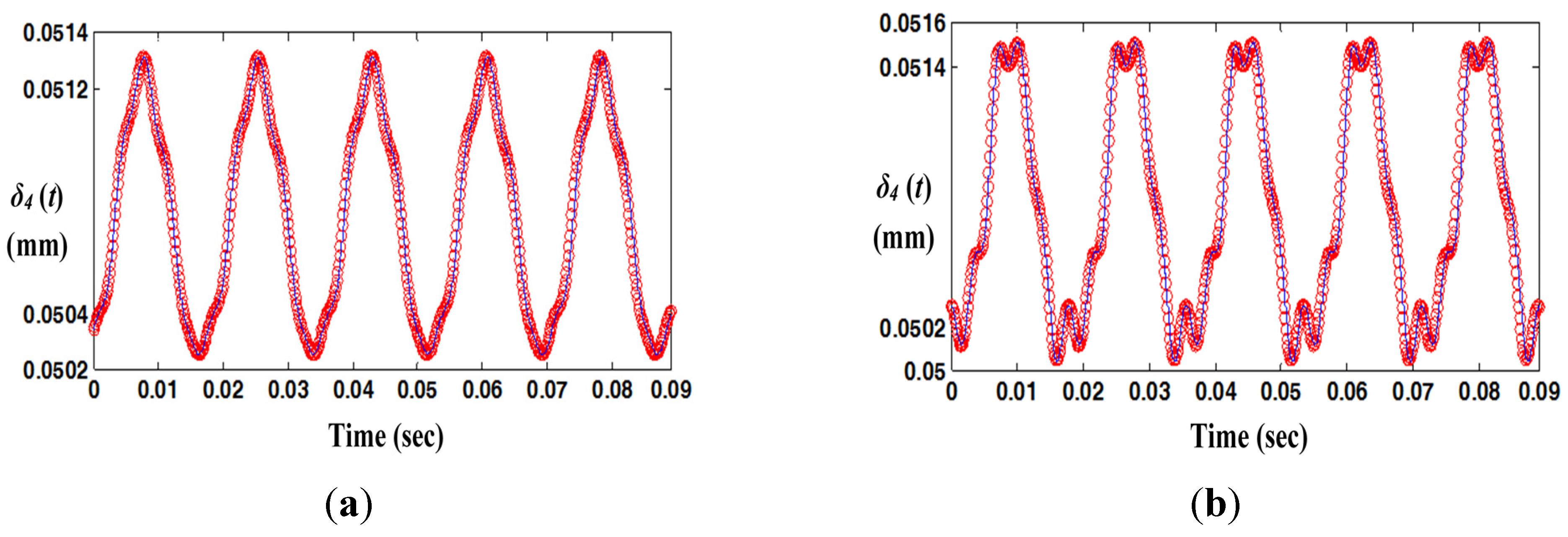
Figure 4 compares the results in the time domain under frequency up- and down-sweeping conditions. By focusing on the normalized frequency
= 0.93 (= 56.5 Hz), where the jumping phenomenon is observed in
Figure 3, the system responses differ considerably depending on the initial conditions and frequency sweeping directions. For example, as shown in
Figure 4b, the dynamic behavior of
δ4(
t) under the frequency down-sweeping condition includes more super-harmonic terms than
δ4(
t) under the frequency up-sweeping condition given in
Figure 4a. This is clearly shown at the peaks of the time history
δ4(
t).
Figure 4.
Comparison of the HBM (
Nmax = 6 and
η = 2) results with the NS results in the time domain at 56.5 Hz: (
a) time histories of
δ4(
t) under frequency up-sweeping; (
b) time histories of
δ4(
t) under frequency down-sweeping. Key:
![Energies 08 08924 i001]()
, HBM;
![Energies 08 08924 i003]()
, NS.
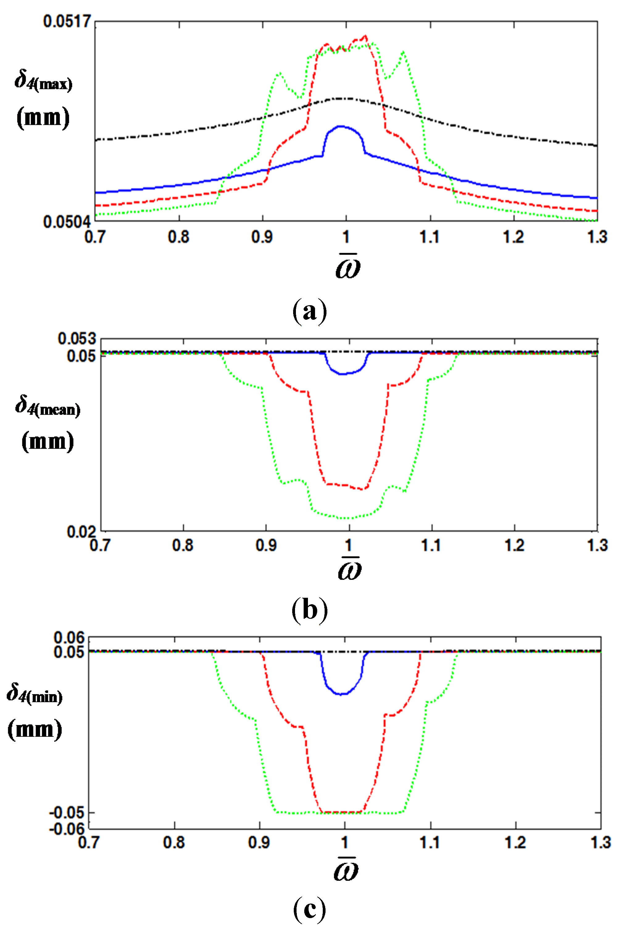
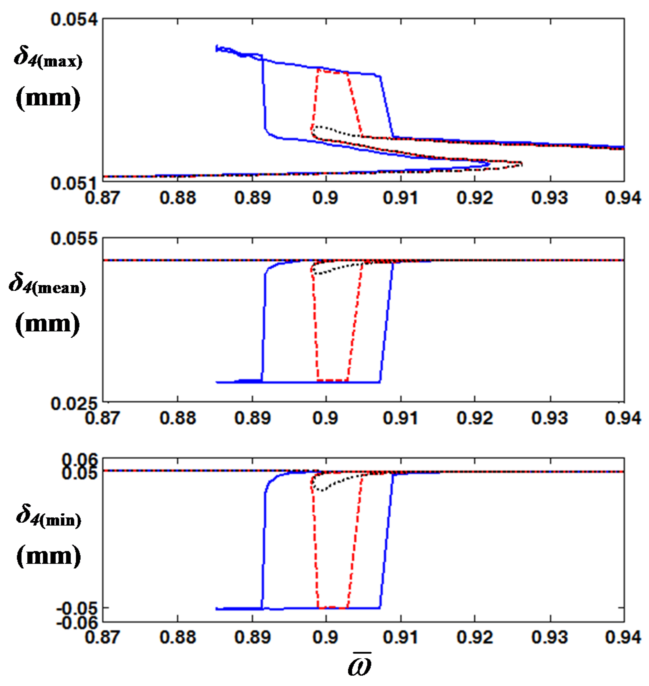
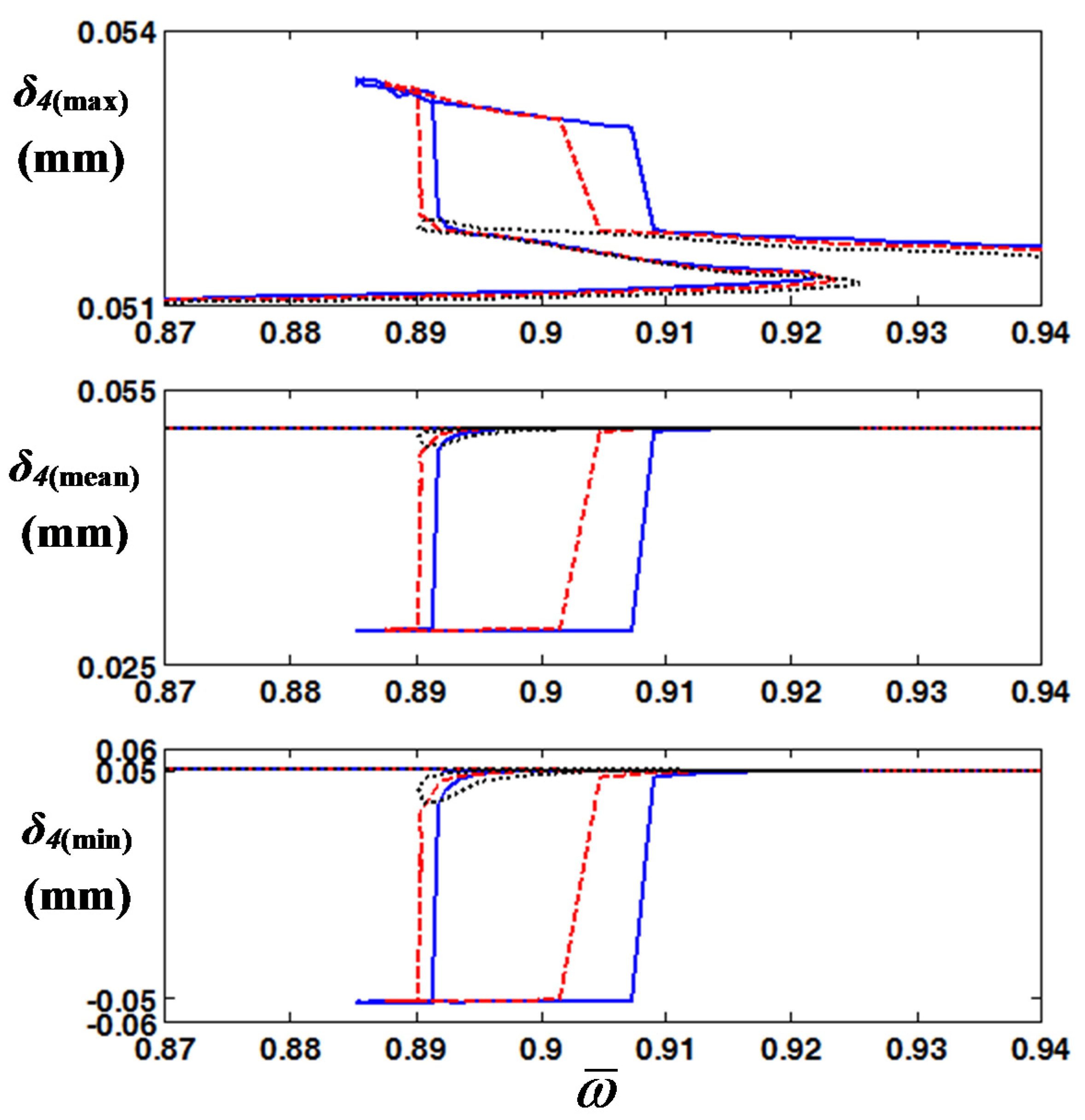
Figure 5 explains the variation in the max, mean, and min values of
δ4(
t) from the HBM in the frequency domain when the number of harmonics is increased. To clearly observe the nonlinear behaviors of gear impact, a damping ratio of 1.3% is used, with which severe impact phenomena such as double-sided impact can be observed [
7,
8]. As shown in
Figure 5, the maxima and minima at resonance and the shape of the backbone are significantly affected by
Nmax. For example, the maximum and minimum values for
Nmax = 1 or
Nmax = 3 along with sub-harmonic index
η = 1 [
9,
22] are considerably smaller than those with
Nmax = 6 and
η = 1 or
Nmax = 6 and
η = 2.
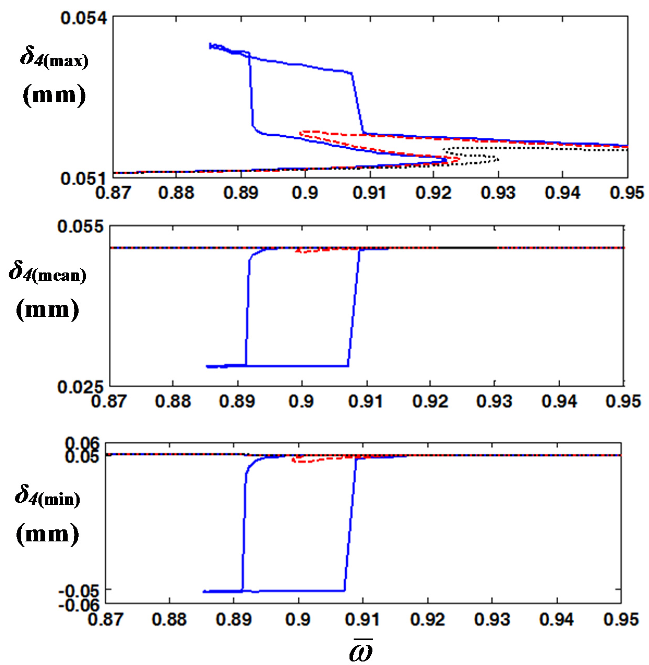
When the jumping phenomena for the gear impact occur, the system response shows considerably different tracks depending on the frequency sweeping directions with
Nmax = 6 and
η = 2, as shown in
Figure 5. When the system is under frequency up-sweeping, the value of the system response
δ4(max) increases following the black dotted line until
reaches a value slightly larger than 0.92.
Figure 5.
Max, mean, and min values of
δ4(
t) from the HBM for 4 cases with different numbers of harmonics: (
a)
δ4(
t)
(max); (
b)
δ4(
t)
(mean); (
c)
δ4(
t)
(min). Key:
![Energies 08 08924 i003]()
,
Nmax = 1 and
η = 1;
![Energies 08 08924 i004]()
,
Nmax = 3 and
η = 1;
![Energies 08 08924 i005]()
,
Nmax = 6 and
η = 1; ─ - ─,
Nmax = 6 and
η = 2.
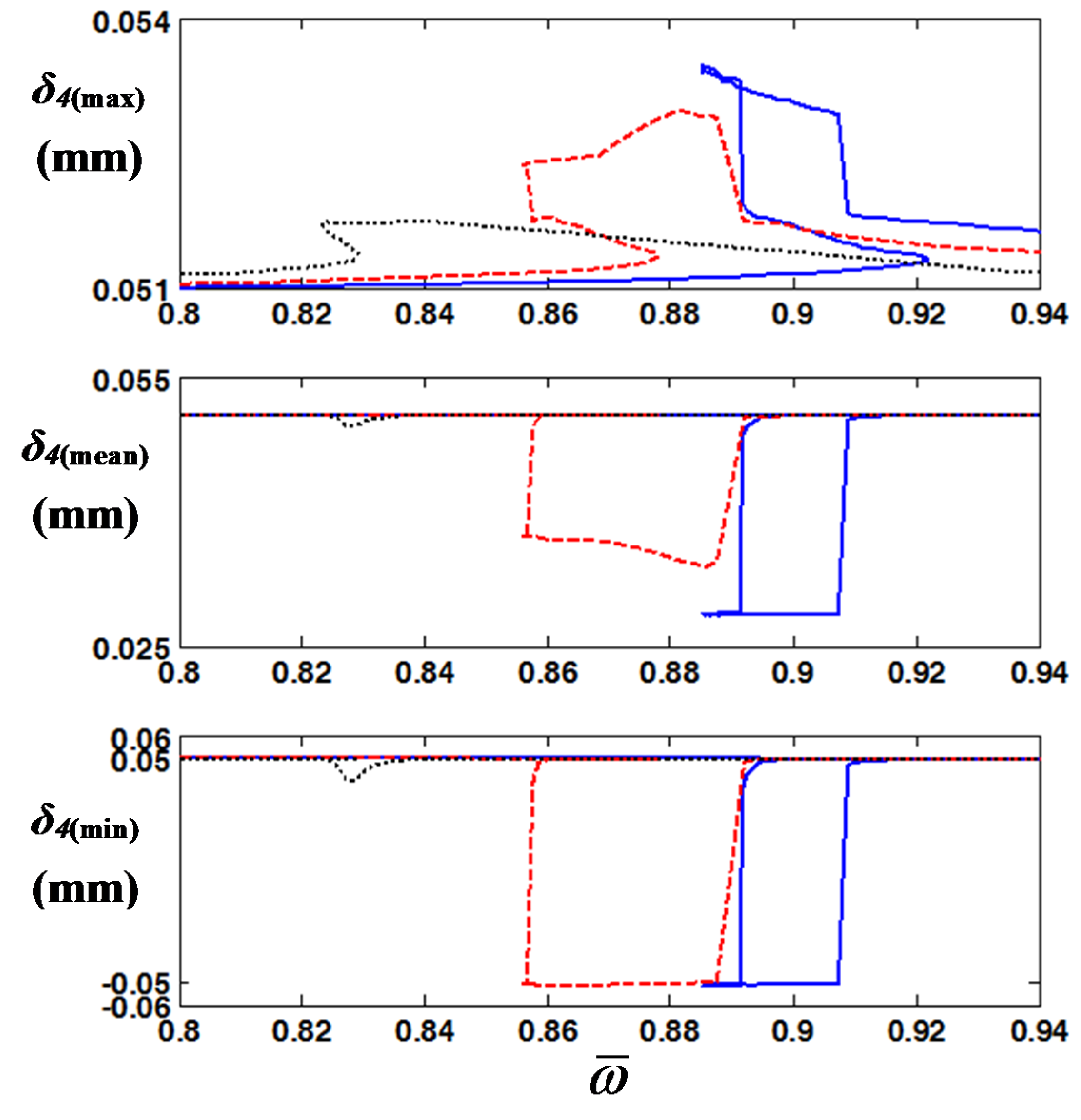
However, under frequency down-sweeping, the system responses have two jumping regimes, where jumping up occurs around
= 0.91 and jumping down occurs around
= 0.885. This dynamic characteristic reflects behavior similar to that observed in a prior study with a single gear pair [
23]. Thus, the simulation results shown in
Figure 5 prove that the gear impact analysis with an individual component can be reasonably extended to the simulation conditions
in situ. In addition, the key factors to reduce the vibro-impacts can be determined easily based on the practical model with six DOF compared with a previously suggested component model [
23]. In the next sections, the criteria with respect to the vibro-impacts will be investigated and discussed based on the simulation results.
4. Impact Pair Analysis with Key Parameters
Gear impacts in a geared system occur under various driving conditions corresponding to the drag torque properties listed in
Table 4 [
7]. The drag torques are estimated based on the results of a prior study [
7,
8] by assuming that the gearbox is operated under different loading conditions, which have significant effects on the drag torque for the vehicle
TDVE2. The other drag torques
TDi,
TDo, and
TDu can be evaluated as suggested previously [
7].
The simulated results for different drag torque conditions are compared in
Figure 6. The results from Case I, II and III show the clear nonlinear impacts compared with Case IV where there is no impact. Case I is estimated by assuming that the vehicle system is operated under normal conditions. Case II involves the gearbox system being affected by double-sided impact. Case III shows the most severe gear impacts compared to the other cases since it shows double-sided impact as well as wider gear impact range. For example, even though Case II shows the same maxima of
δ4(max) and minima of
δ4(min) as Case III, the gear impact range for Case III is wider than for Case II.
Figure 6.
Max, mean, and min values of
δ4(
t) from the HBM for various drag torque conditions: (
a)
δ4(
t)
(max); (
b)
δ4(
t)
(mean); (
c)
δ4(
t)
(min). Key:
![Energies 08 08924 i003]()
, Case I;
![Energies 08 08924 i004]()
, Case II;
![Energies 08 08924 i005]()
, Case III; ─ - ─, Case IV.
Figure 6.
Max, mean, and min values of
δ4(
t) from the HBM for various drag torque conditions: (
a)
δ4(
t)
(max); (
b)
δ4(
t)
(mean); (
c)
δ4(
t)
(min). Key:
![Energies 08 08924 i003]()
, Case I;
![Energies 08 08924 i004]()
, Case II;
![Energies 08 08924 i005]()
, Case III; ─ - ─, Case IV.
With focus on the gear impact, these vibro-impacts are significantly affected by the drag torque values on the unloaded gear
TDu, as shown in
Table 4. Thus, only Case IV overcomes the gear impacts, as shown in
Figure 6. Based on the results, the gear impacts are related to the drag torque of the vehicle and the unloaded gear itself, which extends the gear rattle criteria concepts by including
TDVE2. Thus, it will be clearly shown in the bifurcation diagram in the later section.
Figure 7,
Figure 8,
Figure 9 and
Figure 10 show the results of parametric studies with key property values such as the damping ratio
ζ, clutch stiffness
kC4, and inertias of the flywheel
If and unloaded gear
Iou, given the drag torques of Case IV listed in
Table 4.
Figure 7 compares the HBM results for three modal damping ratios of 1.3%, 1.5%, and 2%. As the damping value increases, the gear impacts are improved from double-sided impact to no-impact conditions [
7,
8,
9]. In addition, the backbone curve can be anticipated with the resonance regimes easily.
Figure 8 shows the effects of the clutch stiffness
kC4 on the gear impacts given the modal damping ratio of 1.3%. When
kC4 is reduced, the gear impacts are improved from double-sided to single-sided impacts. However, changing the stiffness values affects the resonance regimes, because
kC4 is significantly related to the natural frequencies of the torsional system [
7,
8,
22].
Figure 9 and
Figure 10 compare the gear impact conditions for the various inertias of the flywheel and unloaded gear. As clearly shown, increasing the inertia of the flywheel or decreasing the inertia values of the unloaded gear improves the gear impact conditions. Moreover, there are distinct differences in the HBM results in relation to these values. For example, the increase in
If changes the resonance area of
δ4(max),
δ4(mean), and
δ4(min), while the gear impact conditions are improved. However, the reduction in
Iou does not affect the resonance area of
δ4(max),
δ4(mean), and
δ4(min).
Figure 7.
Max, mean, and min values of
δ4(
t) from the HBM (
Nmax = 6 and
η = 2) for 3 values of damping ratio. Key:
![Energies 08 08924 i003]()
,
ζ = 0.013;
![Energies 08 08924 i004]()
,
ζ = 0.015;
∙∙∙∙∙∙∙∙∙∙,
ζ = 0.02.
Figure 7.
Max, mean, and min values of
δ4(
t) from the HBM (
Nmax = 6 and
η = 2) for 3 values of damping ratio. Key:
![Energies 08 08924 i003]()
,
ζ = 0.013;
![Energies 08 08924 i004]()
,
ζ = 0.015;
∙∙∙∙∙∙∙∙∙∙,
ζ = 0.02.
Figure 8.
Max, mean, and min values of
δ4(
t) from the HBM (
Nmax = 6 and
η = 2) for 3 values of clutch stiffness. Key:
![Energies 08 08924 i003]()
,
kC4 = 1838 Nm/rad;
![Energies 08 08924 i004]()
,
kC4 = 1562.3 Nm/rad;
∙∙∙∙∙∙∙∙∙∙,
kC4 = 1279.2 Nm/rad.
Figure 8.
Max, mean, and min values of
δ4(
t) from the HBM (
Nmax = 6 and
η = 2) for 3 values of clutch stiffness. Key:
![Energies 08 08924 i003]()
,
kC4 = 1838 Nm/rad;
![Energies 08 08924 i004]()
,
kC4 = 1562.3 Nm/rad;
∙∙∙∙∙∙∙∙∙∙,
kC4 = 1279.2 Nm/rad.
Figure 9.
Max, mean, and min values of
δ4(
t) from the HBM (
Nmax = 6 and
η = 2) for 3 values of inertia of flywheel
If. Key:
![Energies 08 08924 i003]()
,
If = 0.1376 kg∙m;
![Energies 08 08924 i004]()
,
If = 0.1433 kg∙m;
∙∙∙∙∙∙∙∙∙∙,
If = 0.1434 kg∙m.
Figure 9.
Max, mean, and min values of
δ4(
t) from the HBM (
Nmax = 6 and
η = 2) for 3 values of inertia of flywheel
If. Key:
![Energies 08 08924 i003]()
,
If = 0.1376 kg∙m;
![Energies 08 08924 i004]()
,
If = 0.1433 kg∙m;
∙∙∙∙∙∙∙∙∙∙,
If = 0.1434 kg∙m.
Figure 10.
Max, mean, and min values of
δ4(
t) from the HBM (
Nmax = 6 and
η = 2) for 3 values of inertia of unloaded gear
Iou. Key:
![Energies 08 08924 i003]()
,
Iou = 5.23×10
‒4 kg∙m;
![Energies 08 08924 i004]()
,
Iou = 4.97×10
‒4 kg∙m;
∙∙∙∙∙∙∙∙∙∙,
Iou = 4.61×10
‒4 kg∙m.
Figure 10.
Max, mean, and min values of
δ4(
t) from the HBM (
Nmax = 6 and
η = 2) for 3 values of inertia of unloaded gear
Iou. Key:
![Energies 08 08924 i003]()
,
Iou = 5.23×10
‒4 kg∙m;
![Energies 08 08924 i004]()
,
Iou = 4.97×10
‒4 kg∙m;
∙∙∙∙∙∙∙∙∙∙,
Iou = 4.61×10
‒4 kg∙m.
Overall, based on the HBM results shown in
Figure 7,
Figure 8,
Figure 9 and
Figure 10, the gear impact conditions still follow the previously suggested gear rattle criteria [
7,
8]. The vibro-impact conditions are improved with changes of the resonance regimes and key parameters such as
kC4 and
If based on the HBM, which was not discussed in prior studies. Thus, these parametric studies can give design concepts to avoid gear impacts and system-level vibration problems.
5. Investigation of Bifurcation Diagrams with Focus on Vibro-impacts
Based on the case studies in
Section 4, bifurcation diagrams can be drawn by fixing the specific excitation frequency to
= 0.9 where the double-sided impact occurs. The gear impact conditions can be mapped efficiently by comparing the bifurcation phenomena with gear rattle areas using the values of
δ4(max),
δ4(mean), and
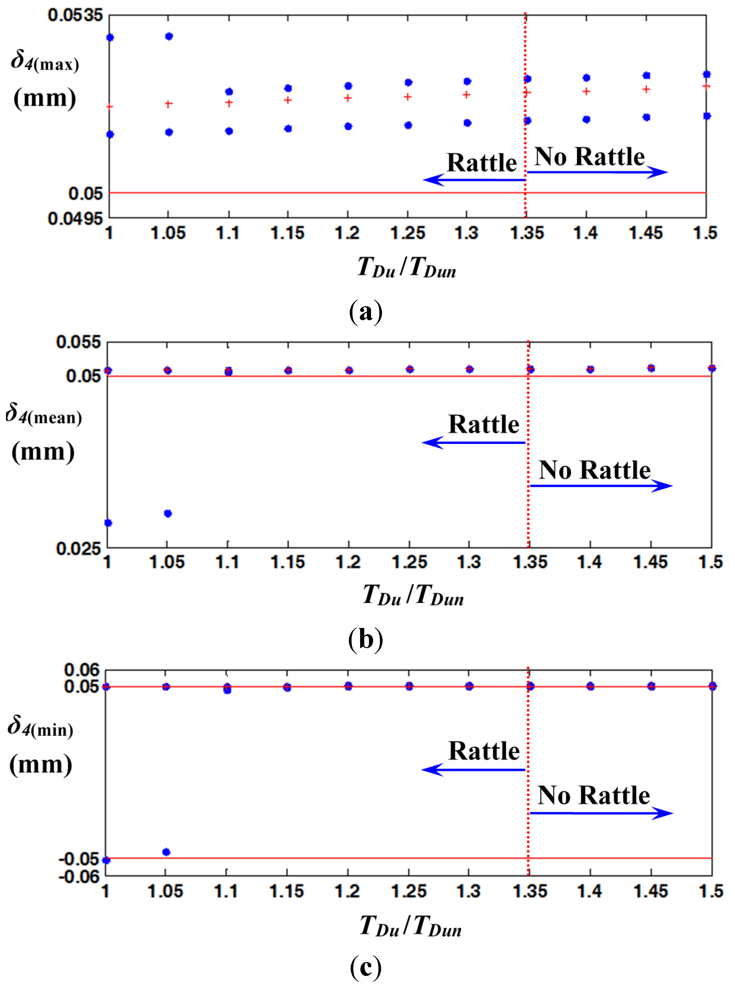
δ4(min). When the gear rattle criteria are determined, “No rattle” indicates frequency areas without any vibro-impacts at any initial conditions. “Rattle” indicates that at least one vibro-impact exists in any condition, either single- or double-sided impact.
Figure 11 includes useful information such as the bifurcation and gear rattle regimes for given drag torques on the unloaded gear
TDun, where the subscript
n indicates the given value of 7.2 Nm for Case IV, as listed in
Table 4.
Here, the unstable values marked by a red cross in
Figure 11 are estimated by employing Hill’s method and the jumping phenomena occur at these areas as shown in
Figure 2 [
2]. Based on the simulated results, when
TDu is increased, the gear impacts decrease and reach the no-impact condition in the region of
TDu /
TDun > 1.35. And this is correlated well with the prior studies [
7,
8]. However, the bifurcation still remains for the entire range of
TDu /
TDun. This means that
δ4(
t) shows considerably different dynamic behaviors depending on the values of
TDu /
TDun and the initial conditions. The red lines in
Figure 11 indicate the marginal area of gear backlash with a value of 0.05 mm at
b/
2 or −0.05 mm at −
b/
2.
Figure 12,
Figure 13 and
Figure 14 show the bifurcation diagrams for the key parameters considered in
Section 4.
Figure 11.
Bifurcation diagrams of max, mean, and min values of
δ4(
t) for drag torque on the unloaded gear: (
a)
δ4(
t)
(max); (
b)
δ4(
t)
(mean); (
c)
δ4(
t)
(min). Key:
![Energies 08 08924 i006]()
, stable value;
![Energies 08 08924 i007]()
, unstable value;
![Energies 08 08924 i008]()
, marginal area of gear backlash.
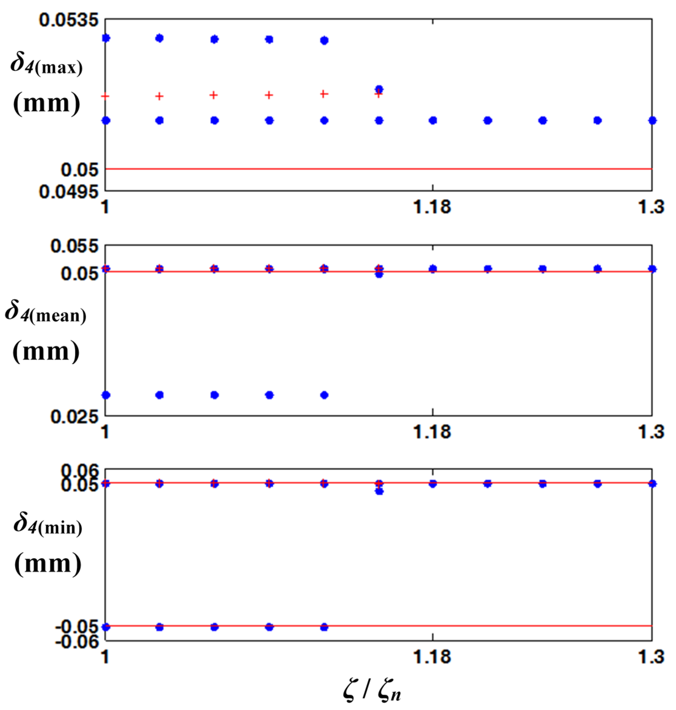
In general, the gear impact phenomena are closely related to the bifurcation regimes, along with the initial or frequency sweeping conditions.
Figure 12 shows the bifurcation results for damping ratios. The employed modal damping
ζn is 0.013, and the bifurcation disappears when
ζ / ζn is greater than 1.18, where the gear impact is also resolved.
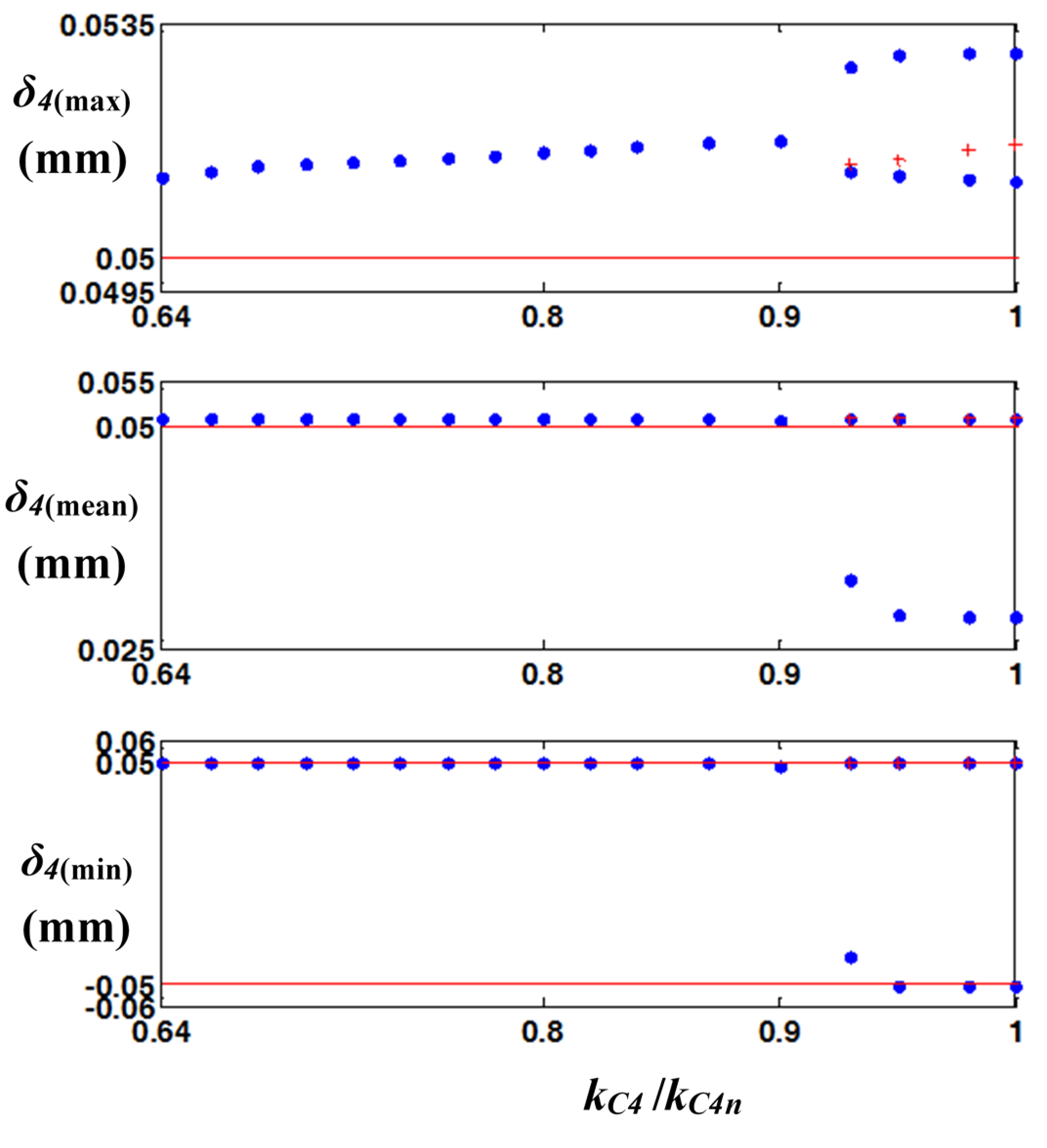
Figure 13 shows bifurcation diagrams for
kC4 /
kC4n, where
kC4n is 1838.0 Nm/rad. The bifurcation disappears when
kC4 /
kC4n is lower than 0.9, and the vibratory problems due to gear impacts are resolved when
kC4 /
kC4n is less than 0.8.
Figure 14 shows bifurcation diagrams for
If /
Ifn, where
Ifn = 1.38×10
−1 kg·m
2. The bifurcation and gear impacts do not occur when
If /
Ifn > 1.05. In contrast,
Figure 15 shows bifurcation diagrams for
Iou /
Ioun with the reverse tendency compared to the bifurcation for
If /
Ifn. For example, the bifurcation and gear impacts disappear when
Iou /
Ioun < 0.66.
Figure 12.
Bifurcation diagrams of max, mean, and min values of
δ4(
t) for damping ratio. Key:
![Energies 08 08924 i006]()
, stable value;
![Energies 08 08924 i007]()
, unstable value;
![Energies 08 08924 i008]()
, marginal area of gear backlash.
Figure 12.
Bifurcation diagrams of max, mean, and min values of
δ4(
t) for damping ratio. Key:
![Energies 08 08924 i006]()
, stable value;
![Energies 08 08924 i007]()
, unstable value;
![Energies 08 08924 i008]()
, marginal area of gear backlash.
Figure 13.
Bifurcation diagrams of max, mean, and min values of
δ4(
t) for clutch stiffness. Key:
![Energies 08 08924 i006]()
, stable value;
![Energies 08 08924 i007]()
, unstable value;
![Energies 08 08924 i008]()
, marginal area of gear backlash.
Figure 13.
Bifurcation diagrams of max, mean, and min values of
δ4(
t) for clutch stiffness. Key:
![Energies 08 08924 i006]()
, stable value;
![Energies 08 08924 i007]()
, unstable value;
![Energies 08 08924 i008]()
, marginal area of gear backlash.
Figure 14.
Bifurcation diagrams of max, mean, and min values of
δ4(
t) for inertia of flywheel. Key:
![Energies 08 08924 i006]()
, stable value;
![Energies 08 08924 i007]()
, unstable value;
![Energies 08 08924 i008]()
, marginal area of gear backlash.
Figure 14.
Bifurcation diagrams of max, mean, and min values of
δ4(
t) for inertia of flywheel. Key:
![Energies 08 08924 i006]()
, stable value;
![Energies 08 08924 i007]()
, unstable value;
![Energies 08 08924 i008]()
, marginal area of gear backlash.
Figure 15.
Bifurcation diagrams of max, mean, and min values of
δ4(
t) for the inertia of the unloaded gear. Key:
![Energies 08 08924 i006]()
, stable value;
![Energies 08 08924 i007]()
, unstable value;
![Energies 08 08924 i008]()
, marginal area of gear backlash.
Figure 15.
Bifurcation diagrams of max, mean, and min values of
δ4(
t) for the inertia of the unloaded gear. Key:
![Energies 08 08924 i006]()
, stable value;
![Energies 08 08924 i007]()
, unstable value;
![Energies 08 08924 i008]()
, marginal area of gear backlash.
Overall, based on the examination of the bifurcation diagrams for the key parameters, the gear impacts can be resolved by adapting relevant parameters, as suggested in prior studies [
7,
8,
9]. Thus, the vibration problems caused by the gear impacts can be resolved by increasing
TDU,
If, and
ζ or decreasing
kC4 and
Iou. Moreover, the bifurcation sometimes does not disappear where the gear impacts are resolved, as shown in
Figure 11, where the bifurcation can be observed for the entire range of
TDu/TDun, including the non-impact region. On the other hand, the bifurcation is directly correlated with the impact phenomena in some cases. For example, as shown in
Figure 15, the bifurcation and gear impact occur (or disappear) at the same
Iou/Ioun.


 , NS by frequency up-sweeping;
  , NS by frequency down-sweeping.

 , NS.
, NS.

 , Nmax = 3 and η = 1;
  , Nmax = 6 and η = 1; ─ - ─, Nmax = 6 and η = 2.


 , stable value;
  , unstable value;
  , marginal area of gear backlash.