Article

Energy Consumption Prediction for Electric Vehicles Based on Real-World Data

by
Cedric De Cauwer
*,
Joeri Van Mierlo
and
Thierry Coosemans
Electrotechnical Engineering and Energy Technology, MOBI Research Group, Vrije Universiteit Brussel, Pleinlaan 2, 1050 Brussels, Belgium
*
Author to whom correspondence should be addressed.
These authors contributed equally to this work.
Energies 2015, 8(8), 8573-8593; https://doi.org/10.3390/en8088573
Submission received: 30 April 2015 / Revised: 30 July 2015 / Accepted: 3 August 2015 / Published: 12 August 2015
(This article belongs to the Special Issue Electrical Power and Energy Systems for Transportation Applications)

Abstract

:
Electric vehicle (EV) energy consumption is variable and dependent on a number of external factors such as road topology, traffic, driving style, ambient temperature, etc. The goal of this paper is to detect and quantify correlations between the kinematic parameters of the vehicle and its energy consumption. Real-world data of EV energy consumption are used to construct the energy consumption calculation models. Based on the vehicle dynamics equation as underlying physical model, multiple linear regression is used to construct three models. Each model uses a different level of aggregation of the input parameters, allowing predictions using different types of available input parameters. One model uses aggregated values of the kinematic parameters of trips. This model allows prediction with basic, easily available input parameters such as travel distance, travel time, and temperature. The second model extends this by including detailed acceleration data. The third model uses the raw data of the kinematic parameters as input parameters to predict the energy consumption. Using detailed values of kinematic parameters for the prediction in theory increases the link between the statistical model and its underlying physical principles, but requires these parameters to be available as input in order to make predictions. The first two models show similar results. The third model shows a worse fit than the first two, but has a similar accuracy. This model has great potential for future improvement.

1. Introduction

The energy consumption of vehicles has been a widely assessed research topic. Until recent years, research was focused on fuel consumption of conventional vehicles, and how driving styles, ITS (Intelligent Transport System) systems, and other intelligent systems impact fuel consumption [1]. Recently, these studies have been extended to the energy use of electric vehicles (EVs). EV energy consumption studies can generally be divided according to their purpose and model calculation methodology. Studies report the development of energy models for the purpose of EV drivetrain design and optimization [2,3], assessment of the influences on the energy consumption [4,5,6], and global energy consumption or grid impact due to the introduction of EV or hybrid vehicles [7,8]. In some cases the energy model is used for an (all-electric) range prediction [9]. The methodology for the calculation of energy consumption either consists of creating a vehicle model that simulates electrical parameters based on kinematic and dynamic requirements (backwards simulation) [3,5,6,7] or by means of statistical models based on measurements of the EV consumption, either from real-world data [4,9] or test cycles [2]. Using real-world measurements has the advantage of predicting more realistic values for energy consumption, but relies on available data and statistical modeling and is often uncoupled from the vehicle dynamics and drivetrain behavior. In contrast, using a vehicle model gives you a direct link with the vehicle dynamics and drivetrain behavior, making the identification of influences of the drivetrain parameters on energy consumption more clear. Although Shankar et al. [4] and Neaimeh et al. [9] both use real-world measurements for the calculation of the energy consumption, only a limited number of external parameters are included in their models and the link with the vehicle dynamics is low. In Neaimeh et al. [9], the prediction was based on a simplified vehicle dynamics model and only included road inclination as an external influencing parameter, whereas Shankar et al. [4] use a purely statistical approach based on road type detection and its linked average consumption. This paper proposes to extend those models and fill this knowledge gap by including more external parameters while increasing the link with the vehicle dynamics. The goal here is to detect and quantify correlations between the kinematic parameters of the electric vehicle and its energy consumption using real-world data, in order to predict the real-world consumption of electric vehicles as an intermediate step towards range prediction. A model that uses real-world data compared to using cycle test values produces more realistic energy consumptions, and has added value for research topics relying on consumption data as input. Life Cycle Assessments (LCA) and Total Cost of Ownership (TCO) studies, for example, still use energy consumption based on the New European Drive Cycle (NEDC) [10,11,12] or other standardized cycles.

2. Energy Models

The goal is to build up EV energy consumption models based on real-world measurements. The proposed models are statistical models based on the underlying physical principles of the vehicle dynamics and kinematics. As the ultimate goal of this study is all-electric range (AER) prediction for electric vehicles, the energy consumption considered in this paper is the energy consumption on a battery-to-wheel scope as defined in De Cauwer et al. [13] and corresponds to the energy drawn from the battery. Therefore, energy losses in the energy supply chain prior to the battery are not considered as they do not impact the range of the EV. As such, grid losses and charging losses are not included in this model. As De Cauwer et al. [13] argues, it does, however, influence real-world tank-to-wheel consumption and therefore the costs associated with real-world EV use. The battery-to-wheel consumption of an electric vehicle is a function of the required mechanical energy at the wheels, determined by the kinematic parameters over a trajectory, the drivetrain efficiency, and the energy consumption of auxiliaries. The total required mechanical energy at the wheels as a function of the kinematic parameters describing vehicle movement can be expressed in the vehicle dynamics equation:
E i j = 1 3600 [ m i j . g . ( f . c o s φ + s i n φ ) + 0.0386. ( ρ . C x . A . v i j ² ) + ( m i j + m f ) . d v d t ] d i j ,
where:
E i j = Mechanical energy required at the wheels to drive on a distance   d i j   [ kWh ] m i j = Total vehicle mass   [ kg ] m f = Fictive mass of rolling inertia   [ kg ] g = Gravitational acceleration   [ m / s 2 ] f = Vehicle coefficient of rolling resistance   [ - ] φ = Road gradient angle   [ ° ] ρ = Air density   [ kg / m 3 ] C x = Drag coefficient of the vehicle   [ - ] A = Vehicle equivalent cross section   [ m 2 ] v i j = Vehicle speed between the point   i   and the point   j   [ km / h ] d i j = Distance driven from point   i   to point   j   [ km ]
Equation (1) includes five terms, each describing a contribution to the energy consumption. These terms describe, respectively, the rolling resistance, potential energy, aerodynamic losses, kinetic energy, and energy for the acceleration of rotational parts. The aerodynamic losses and rolling resistances are pure energy losses. The potential and acceleration (kinetic) energy for EVs, unlike for conventional vehicles, can partly be recovered by regenerative braking. It is the EV battery that provides, through the numerous energy conversion steps of the drivetrain, the required energy for traction. Additionally, the EV battery also provides the energy to supply the auxiliaries. Heating and air-conditioning systems can make a significant contribution to the EV energy consumption and are ambient temperature dependent.
The proposed models are statistical models that correlate these kinematic parameters over a trajectory and the measured energy consumption at the battery, based on the vehicle dynamics equation. They are application specific, because different research topics do not necessarily have the same input data available for the model, nor do they require the same level of accuracy. Three models will be proposed here: one using the aggregated trip data, a second using aggregated trip data with additional acceleration data, and a third using shorter trip segments or “micro-trips” to calculate energy consumptions. These models have a direct link with the vehicle kinematics (vehicle speed, distance, altitude, etc.) but do not yet allow extraction of secondary effects that impose kinematic constraints (such as traffic and weather), although this information is inherently included in the real-world data.The first energy model is a model based on macro trips, i.e., uses aggregated values of the kinematic parameters that describe trips. These are the average vehicle speed, the distance driven, and the elevation. By applying multiple linear regression on the real-world measured values of the consumed energy and kinematic parameters for trips, a linear model is created based on the vehicle model presented above. The model presented in Lebeau et al. [14] used the vehicle dynamics equation to calculate the required mechanical energy and added a temperature- and time-dependent term to account for auxiliaries and temperature-dependent efficiencies. The difference here is that the prediction is purely statistical without any calculation based on theoretical values, and based on the underlying known relations between energy consumption and a number of independent variables presented in Equation (1). As such we must have a distance-dependent term describing rolling resistance, a speed-squared-dependent term describing aerodynamic losses, a height-dependent term describing potential energy, and a term describing auxiliary consumption. Two obvious factors influencing energy consumption that are present in the physical model, i.e., acceleration and weight variation, are absent here. This approach is justified for applications where the input data for the prediction only contain aggregated values of the kinematic parameters (such as those presented in Lebeau et al. [14]). The weight factor cannot be extracted as this information was not in the available data. To describe the linear dependency of the auxiliary use and the energy consumption, we introduce a temperature-scaled, time-dependent term. To be able to introduce such a term into the linear regression, we reform the temperature scale to an absolute one, with 20 °C being the neutral temperature, and introduce the parameter aux ∊ [0,1], with its value being the ratio of the time the auxiliaries are on. Now the independent variable in the regression analysis describing auxiliary consumption becomes:
| 20 T | a u x t
with:
T : a m b i e n t   t e m p e r a t u r e   i n   ° C   t : t i m e   d i f f e r e n c e   a u x :   D u r a t i o n   o f   a u x i l i a r i e s   s w i t c h e d   o n T o t a l   d u r a t i o n   o f   t r i p
The resulting formula using linear regression describing energy consumption in this simplified model then becomes:
E = B 1 s + B 2 v 2 s + B 3 | 20 T | a u x t + B 4 H p o s + B 5 H n e g + ε
with:
B i : r e g r e s s i o n   c o e f f i c i e n t s   E : e n e r g y   v : average speed  s : d i s t a n c e | 20 T | a u x : s c a l e d   t e m p e r a t u r e   v a l u e   w i t h   T   i n   ° C   t   : t i m e   H p o s : p o s i t i v e   e l e v a t i o n   H n e g : n e g a t i v e   e l e v a t i o n   ε :   e r r o r   t e r m
Except for the temperature, the unit of each parameter does not matter as a linear relationship is assumed; it will only change the regression coefficients but not the result. This model will be referred to as the macro model. Using the average speed instead of the integration in the aerodynamic term ( B 2 v 2 s ) in Equation (3) (or sum because of the discrete nature of the data) introduces a (large) approximation because of the quadratic nature of the term. Moving towards a model that is no longer restricted by the available input data for prediction, the aerodynamic term in Equation (3) can be replaced by:
B 2 i = 1 n v i 2 s i  
with:
i = 1 n s i = s
where n is the number of recorded data points.
Similarly, the v i can be used to include a term describing acceleration, so kinetic energy changes are calculated by the sum of the squared speed differences. If divided by the distance driven, this becomes a characteristic metric that is here called the constant motion factor (CMF) and describes the kinetic energy changes per unit distance:
C M F =   i = 2 n | v ² i v ² i 1 |   s  
Over a complete trip there will be as much positive change as negative change and the contributions of decelerations and accelerations to the CMF will be virtually equal. Including Equations (5) and (6) in Equation (3) gives:
E = B 1 s + B 2 i = 1 n v i 2 s i + B 3   abs ( 20 T )   aux   t + B 4 i = 2 n | v ² i v ² i 1 |   s i + B 5 Hpos + B 6 Hneg + ε = B 1 s + B 2 i = 1 n v i 2 s i + B 3 | 20 T |   aux   t + B 4   CMF   s + B 5 Hpos + B 6 Hneg + ε
This model uses non-averaged data of the speed and distance parameters and sums them up over the trip before performing the linear regression on the aggregated values. The model and its coefficients are still based on the aggregated trips but not yet based on micro-trips. Therefore we will refer to this model as the hybrid model.
Another option is to segment a trip into pieces of equal duration (micro-trips) and use the detailed measuring points to make a prediction on the micro trip consumption using linear regression. Thereafter the consumptions of the segments are integrated over the trip to predict the total consumed energy. Unlike for the macro trips, for the micro trips the contributions of the positive and negative speed changes to the CMF will not necessarily be equal and the CMF should be split in CMF+ and CMF when vi+1 > vi and vi+1 < vi respectively.
In this model, Equation (7) evolves to:
E = E m i c r o = s e g m e m t s t r i p B 1 i s e g m e m t s i + B 2 i s e g m e m t v i 2 s i + B 3 | 20 T s e g m e m t | a u x s e g m e m t t s e g m e m t + B 4 ( i s e g m e m t C M F i + ) s + B 5 ( i s e g m e m t C M F i ) s + B 6 i s e g m e m t H p o s i + B 7 i s e g m e m t H n e g i + ε
This model has the potential to be the most accurate as it does not apply averaging and so more information resides in the values of the parameters. However, these detailed values of the kinematic parameters to be fed into the model for prediction are not necessarily readily available for any random trip, making prediction with this model impossible. To make this model applicable for the prediction of energy consumption of new trips, an additional correlation has to be done between characteristic values of these kinematic and physical (measured here) parameters and external factors so that their occurrence in the chosen trip can be predicted. This model will be referred to as the micro model.

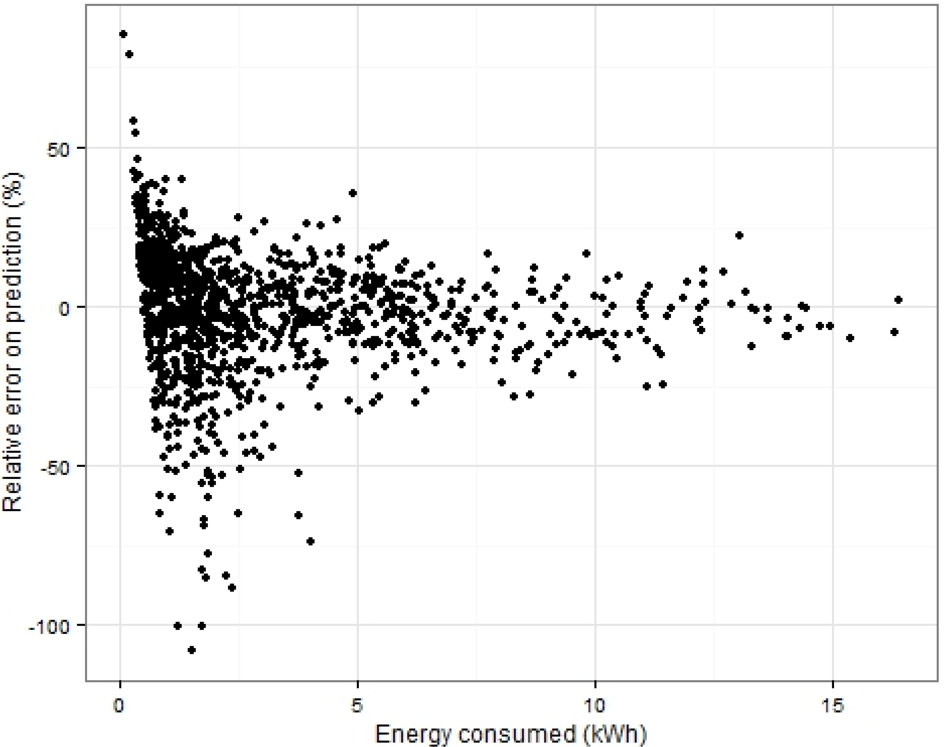
3. Data Availability and Reliability

The available data were generated with a logger device recording the CAN bus signals of a 2012 Nissan Leaf (24 kWh Li-Ion battery, 80 kW electric motor, 1700 kg vehicle mass [15]) during a two year period of 2013 and 2014. A CAN logger registered the battery current and voltage, the state-of-charge (SoC), the GPS coordinates, and the timestamp at a 1 Hz frequency. This provided a dataset containing 23,700 km distance covered, spread over the 261 days in 2013 and 312 days in 2014 when the vehicle was driven (out of a total of 730 days registered). The vehicle was driven by up to 10 individuals on a regular basis, with no restrictions of use, and was located in the outer region of the city of Brussels. This way most types of use and road topology (urban, highway, rural, 
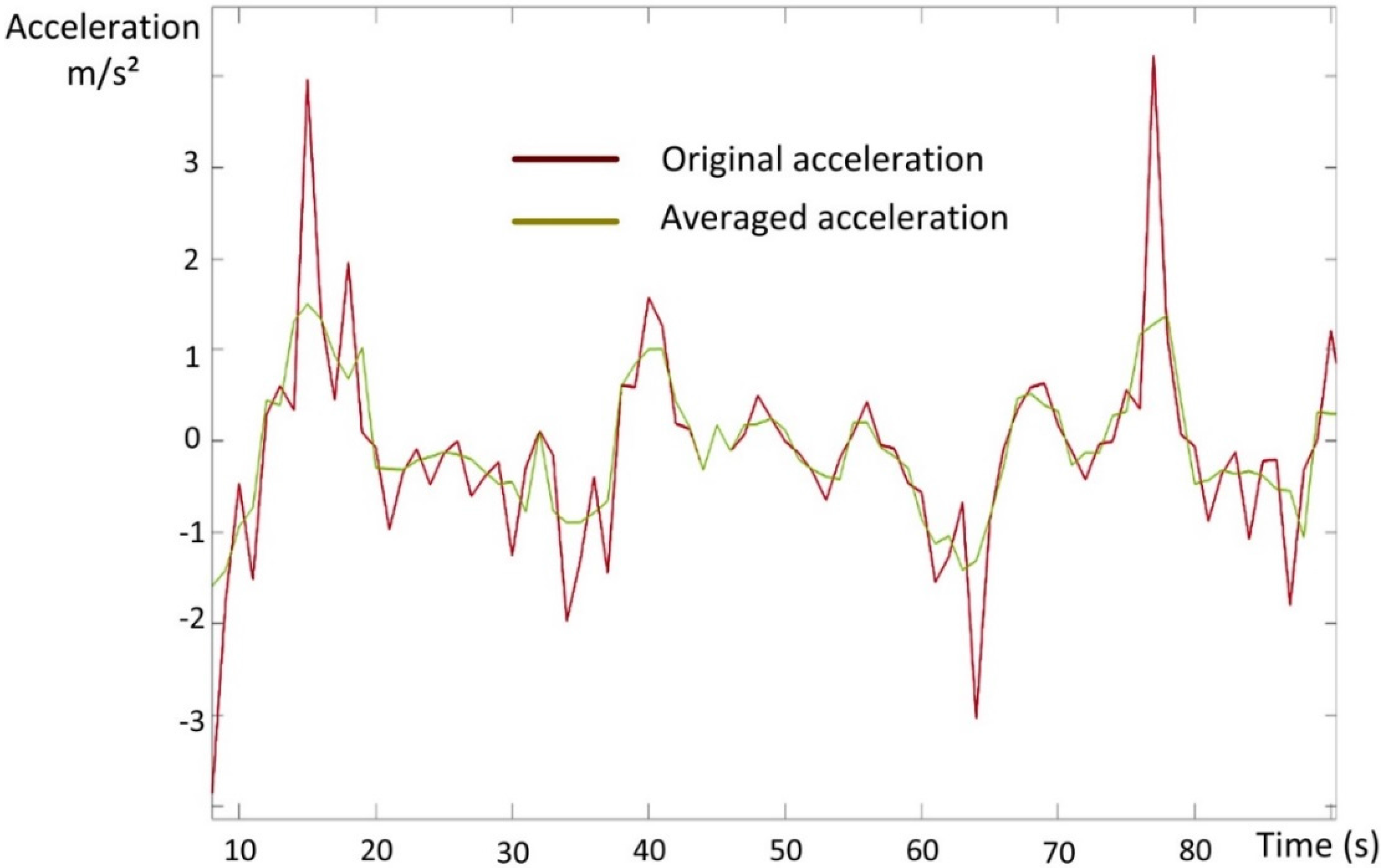
etc.) are represented in the data. However, because the data are generated by only one vehicle, the constructed models are drivetrain specific and potential differences in the impact of the external factors on real-world energy consumption for different EV types cannot be extracted from the data. The speed and acceleration values used are based on position coordinates; therefore an error exists on speed and especially acceleration. The acceleration often showed unrealistic acceleration peaks of over 2 m/s². Therefore, if the speed was monotonically increasing (positive acceleration) or decreasing (negative acceleration) over multiple measurement points, the acceleration was averaged up to a maximum of three measurement points (3 s). By increasing the duration over which the acceleration is calculated, the relative error of the acceleration decreases, but the acceleration is more averaged. The maximum of three measurement points (so 3 s) was chosen to have a balance between both. The acceleration peaks and the averaged values are illustrated in Figure 1 by plotting the acceleration values for 2014 for a selection of data points.
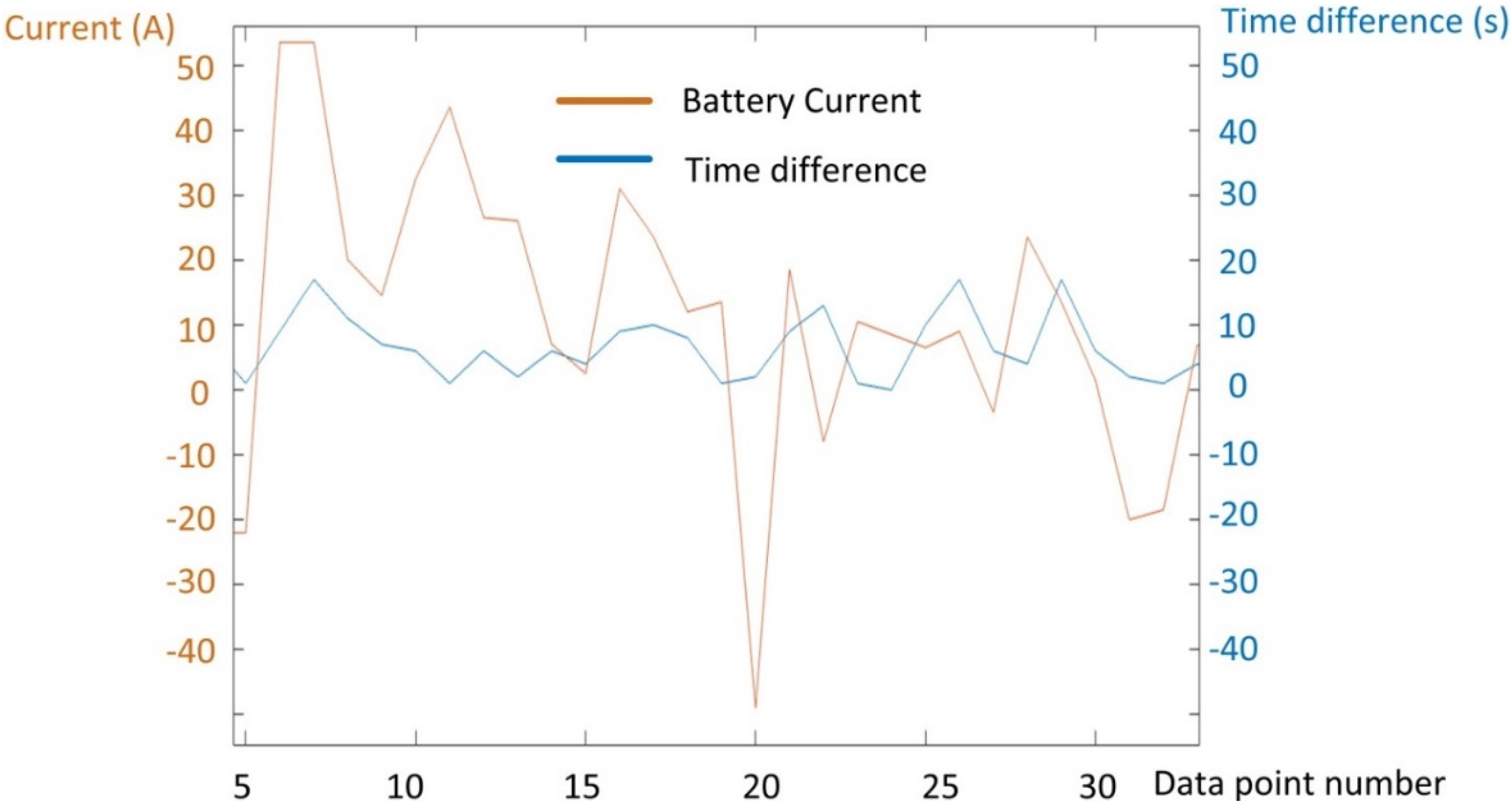
Occurrences of loss of satellite connection caused the data to “jump”, i.e., divert from the 1 Hz data point registration. Because of this, the vehicle “jumps” to the next location, making the distance between the points the straight line distance, causing the distance and acceleration to be wrong. Moreover, as the energy consumption is calculated by integrating the battery voltage and current over time, decreasing the log frequency increases integration error. This effect can be considerable when driving into tunnels. Making a hard filter to eliminate all trips that recorded events of time lapses over 3 s resulted in only 15%–30% of the total available trips remaining. Investigation of these particular trips with time lapses showed they did not significantly alter the results of the models on a systematic basis. Therefore, when using the data structured under the form of trips, we decided not to use this hard filter but to eliminate individual cases (entire trips) after analysis using statistical post-processing tools: extreme values of the standard residuals (>2) and Cook’s distances (>1) were individually investigated and eliminated in the case of non-reliable data. Figure 2 shows a part of a trip where time lapses are registered. It also shows the current value at those points to illustrate that data jumps at non-average current values lead to large energy errors due to the integration.
Figure 1. Acceleration and averaged acceleration for a number of data points.
Energies 08 08573 g001
An additional problem was the occasional speed spike. The trips containing unrealistic high speed values were deleted a posteriori after detection of outliers through the same statistical post-processing tools. After the post-processing and filtering was applied, the remaining usable data for the model construction consisted of 21,300 driven kilometers. All the remaining usable data was used for the multiple linear regression and not split up into parts for model construction and model validation. The statistical nature of the model, the vast amount of measured data used, and post-processing sensitivity analysis justify this approach. However, for further improvement and usefulness of the model, the considered vehicle fleet could be extended and further validation of the individual contributions of external factors could be performed.
Figure 2. Example of data point jumps and the current value at those points.
Energies 08 08573 g002

4. Model Results

4.1. Macro Models

The results of the multiple linear regressions for both the macro model and hybrid model are presented in Table 1. The table gives the correlation coefficient (R2), an overview of the regression coefficients (Bi) and its standard deviation (SE Bi) and confidence level (P), the standardized beta estimates (βi), and the relative average contribution of each term. The standardized beta estimates give the number of standard deviations by which the prediction will change when the predictor changes one standard deviation and is, as such, an indication for the importance of a predictor. The relative average contribution of a term (expressed as a percentage) is the contribution of that term to the total energy consumption and is calculated by taking the sum over all trips of that term, multiplied by its regression coefficient and then divided by the sum of all energy consumption.
The confidence levels of the regression coefficients show that all predictors are very significant. The relative average contribution is an indication of how each predictor (term) contributes to the total energy consumption. The difference of the relative average contributions and standardized beta coefficients for the different predictors between the macro and hybrid model shows that the model is sensitive to the presence or absence of significant predictors. Introducing the CMF to include acceleration in the model has a big impact on the regression coefficients and thus the average contribution of the terms to the total consumption. The acceleration term accounts for almost 20% of the energy consumption, mostly at the cost of the rolling resistance contribution, which decreases by 25%. Introducing an acceleration term also causes minor shifts in the other terms. It is, however, logical that with the absence of an acceleration term in the macro model, the contribution of the acceleration shifts to the distance term because, on average, longer trips will have more acceleration actions. However, on individual trips, this is not the case at all because for trips with an equal distance, the amount and magnitude of acceleration actions can vary significantly depending on the road type, congestion level, and driving style. In both models a constant term also makes a contribution to the prediction. These constant terms come out of the linear regression, but were not defined in the physical model. This means part of the variability of the data is not accounted for by the predictors from the physical model and resides in this intercept term. One cause can be the non-linear auxiliary consumption during trips, which is caused by the conditions of the vehicle after a period of standstill. After a period of standstill, the vehicle first has to be brought to the requested temperature before maintaining this temperature for the rest of the trip, during which the consumption can be expected to be linearly time dependent. Although average contributions of the intercept terms are small for both models (3%–4%), the contribution per individual trip can be much higher. The average contribution is a good measure of how much each term contributes to the total energy consumption but gives no information on the distribution of contributions across the trips. There are considerable variations in the relative contribution of each term to the consumed energy across these trips. For the constant term, for example, the absolute contribution will be the same for a very short or very long trip, making the relative contribution vary strongly. For the auxiliaries, the distribution of contributions also includes trips with no auxiliary use, thus pulling the average value down. To illustrate these examples, the distributions of the contribution to the energy consumption per trip by the auxiliary and constant term resulting from the model are shown in Figure 3 and Figure 4, respectively.
Table 1. Multiple linear regression results for the macro and hybrid model.
Adjusted R2BiSE BiβiPAvg. % Contribution
Model 1 macro0.956 <0.001
Constant 1.19E-12.65E-2 <0.0014%
Rolling resistance 1.32E-11.84E-30.83<0.00178%
Aerodynamic 5.00E-64.45E-70.11<0.0016%
Auxiliaries 1.83E-17.35E-30.14<0.0017%
Pos. elevation 3.08E-33.72E-40.23<0.00126%
Neg. elevation −2.54E-33.68E-4−0.19<0.001−21%
Model 2 hybrid0.968
Constant 9.24E-22.33E-2 <0.0013%
Rolling resistance 9.36E-22.40E-30.58<0.00155%
Acceleration 1.00E-27.53E-30.16<0.00118%
Aerodynamic 5.59E-62.35E-70.24<0.00115%
Auxiliaries 1.78E-16.28E-30.14<0.0017%
Pos. elevation 2.75E-33.18E-40.21<0.00123%
Neg. elevation −2.59E-33.15E-4−0.20<0.001−22%
R2: correlation coefficient; Bi: regression coefficient; SE Bi: standard deviation of the regression coefficient; βi: standardized beta estimate; P: confidence level; Avg. % contribution: the relative average contribution.
Figure 3. Distribution of the relative contribution of the auxiliary term to the energy consumption of all trips.
Energies 08 08573 g003
Figure 4. Distribution of the relative contribution of the constant term to the trip consumption for all trips.
Energies 08 08573 g004
The distribution of the contribution of the auxiliaries to the energy consumption given by the model is hyperbolic, with a spike for non-auxiliary use trips and contributions running up to about 80% (rare occasions). The trips with a prediction of a high relative contribution of the auxiliary energy consumption are trips with low average speed. Relative contributions of the auxiliary consumption for trips with an average speed of over 40 km/h do not exceed 40%. A low average speed means a low average power demand (or increased standstill periods), increasing the auxiliary consumption relative to the total consumption. This effect is most noticeable in this simple macro model, where the contribution of the accelerations is not accounted for and this driving characteristic is only represented in the speed-dependent (quadratic) aerodynamic term. This shows how a different use of the vehicle results in significantly different energy consumption. The distribution of the constant term contribution to the energy consumption prediction is a direct result of the distribution of the trip consumptions and ranges up to almost 25%.
Using R to construct the 0.99 confidence interval for the predicted value, then dividing those values by the predicted value gives the confidence interval on the prediction relative to the value itself. The results are shown in Figure 5. For trips over 5 kWh, the 0.99 confidence interval remains within 5% of the predicted value, meaning that the distributions of the regression coefficients are narrow and very significant and the average of those predictions are statistically not likely to be more than 5% off. Looking at the actual relative error on the prediction (that is, the measured value minus the predicted, divided by the measured value), errors can be quite large for trips with a low quantity of energy consumed (<2.5 kWh), although the concentration of trips remain within the 25% error margin. The relative error on the prediction for the macro model and its distribution can be seen in Figure 6 and Figure 7, respectively. The graph in Figure 6 also shows that the average relative error decreases for trips with a higher quantity of energy used and stays within the 25% error band for trips higher than 2.5 kWh consumption (except for a few negative errors). This band narrows further with increased consumption.
Figure 5. Confidence intervals for the predicted values of the macro model, expressed in relative distance (%) to the predicted value.
Energies 08 08573 g005
Figure 6. Relative error prediction (%) as a function of the consumed energy (kWh) in the trip for the macro model.
Energies 08 08573 g006
Figure 7. Distribution of the relative errors (%) for the macro model.
Energies 08 08573 g007
The plot of relative errors of the hybrid model has a very similar shape to the macro model, but with lower errors and an error band that narrows down more quickly with increased energy consumption trips, as can be seen in Figure 8.
Figure 8. Relative error on the prediction (%) as a function of the consumed energy (kWh) in the trip for the hybrid model.
Energies 08 08573 g008

4.2. Micro Model

The results of the hybrid model show that moving towards more detailed values of the predictors shifts the regression coefficients and results in a better correlation. A next step can be dividing the trips into smaller segments to build the regression model, and then aggregating the predictions of the energies for the segments to obtain the energy consumption of a considered trip. Using this approach, detailed values of the kinematic parameters, instead of averaged or aggregated values, are required to be able to calculate the predictor values over segments, making this model unusable for cases where these data are not available. Yet, if it is possible to link characteristic values of these predictors to known parameters, such as congestion levels and road type, this approach has great potential for improving the above model. Following this logic, these segments need to have sufficiently significant values for the predictors but avoid over aggregation. Therefore trips have been segmented into blocks with an equal duration of 2 min, 5 min and 10 min for experiments with the magnitude of the blocks, starting with 2 min segments. The results of the multiple linear regression using 2 min micro-trips are listed in Table 2.
Table 2. Results of the multiple linear regression for the micro-trip model.
Adjusted R2BiSE BiβiPAvg. % Contribution
Model 3 Micro0.89
Constant 3.38E-21.49E-3 <0.00118%
Rolling resistance 6.43E-21.80 E-30.35<0.00135%
Acceleration (pos) 3.14E-33.81E-30.52<0.00159%
Acceleration (neg) 1.98E-33.87E-30.33<0.001−136%
Aerodynamic 7.85E-61.58 E-70.41<0.00117%
Auxiliaries 1.94E-23.44E-30.22<0.0019%
Pos. elevation 1.05E-34.01E-50.12<0.00111%
Neg. elevation −1.16E-33.99E-5−0.13<0.001−12%
Again, all predictors are very significant. The relative average contributions of the auxiliaries’ term, aerodynamic term, and acceleration term are very similar to the hybrid model, but other contributions are different. The 2 min segment model showed the following problems:
  • A large contribution of the constant (error) term (20% on average);
  • A bigger negative contribution of the negative elevation than the positive contribution of the positive elevation, which does not correspond to the physics;
  • Low correlation coefficient (around 0.89).
This resulted in a process of detailed investigation to find the reasons for these problems and how to solve them. The problems were not caused by an insufficient number of data points per segment, as increasing the segment duration (and thus the level of aggregation) did not resolve this problem. One way of solving the problem is to combine a dataset of 2 min segments with a dataset of 10 min segments. This led to results that correspond to the physical principles of the model, yet are statistically unsound because of the artificial distribution of energy consumptions with the two levels of duration. Therefore the two min segment seems the best choice and gave the best results. However, the problems listed above demonstrate that a lot of the variability in the data is not accounted for by the model. The suspected reason for this is that because of the low predictor values, the errors in the measurements (such as integration error, assumptions in Equation (2), etc.) become more significant and influence the linear regression. The relative error on the prediction of the micro-trips (segments) and its distribution are depicted in Figure 9 and Figure 10, respectively. The figures show that large error exists for the prediction segment energy consumption, but the bulk of the error lies within the 25% error band. The existence of large error for the segment predictions is consistent with the observation above that less variability is accounted for in the micro model. Combining the micro segment predictions, the energy consumption for the trips can be calculated. The relative error on that prediction is given in Figure 11. Despite the flagrant problems with the model listed above, it shows comparable accuracy to the macro and hybrid model for the prediction of energy consumption of complete trips.
Figure 9. Relative errors on the micro-trip energy consumption predictions using the micro model.
Energies 08 08573 g009
Figure 10. Distribution of the relative errors on the micro-trip energy consumption predictions using the micro model.
Energies 08 08573 g010
Figure 11. Relative error in the trips’ energy consumption predictions using the micro model.
Energies 08 08573 g011
Comparing Figure 11 with Figure 6 and Figure 8 demonstrates that the micro model accuracy is similar to the accuracy of the macro and hybrid model, with errors drastically decreasing when the quantity of consumed energy is above 2.5 kWh and is within the 25% error band for most of the trips.
Another approach would be to split up the energy consumption into positive (tractive power) and negative (regenerative braking) power, and construct a linear model for the regenerative energy with the negative acceleration and elevation. Using this approach, however, the negative elevation turns out not to be a significant parameter. This is not illogical, as gentle elevation differences do impact the positive power (tractive effort required) but do not necessarily result in negative power, as is further discussed in Section 5.

5. The Regenerative Braking Influencing Factors

Regenerative braking for EVs is an important part of the EV drivetrain efficiency [16] and regenerative braking strategies are a topic of research [16,17,18]. 
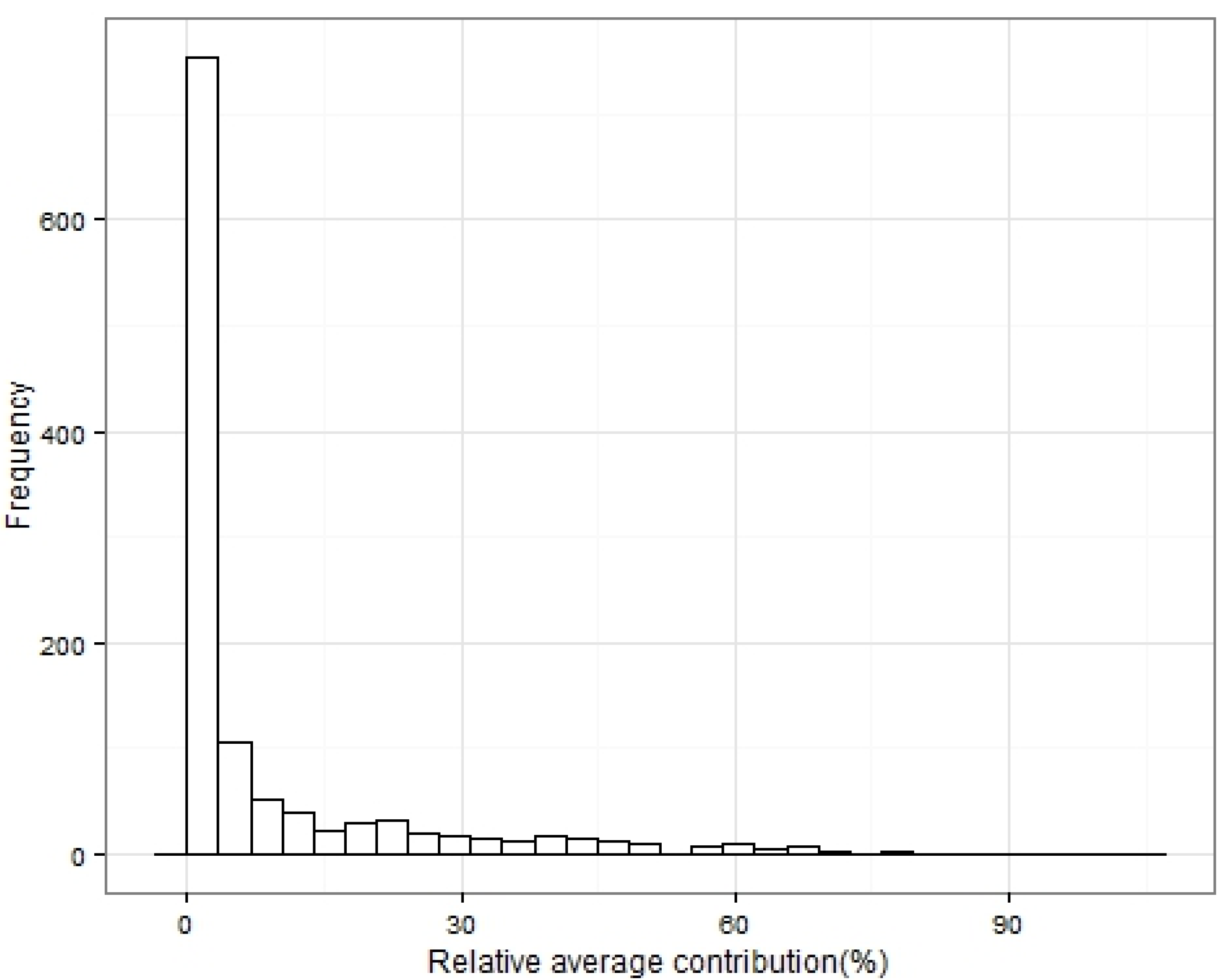
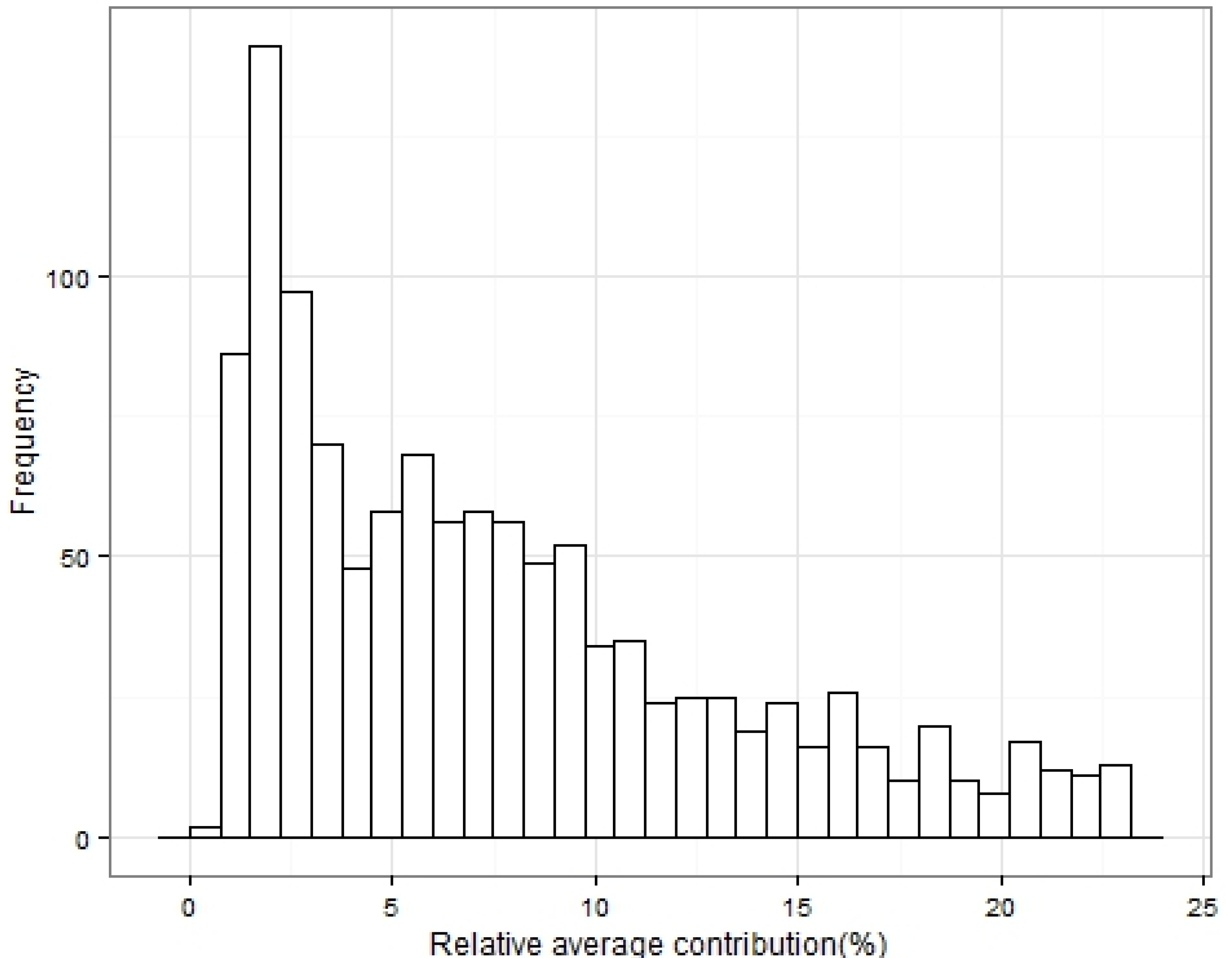
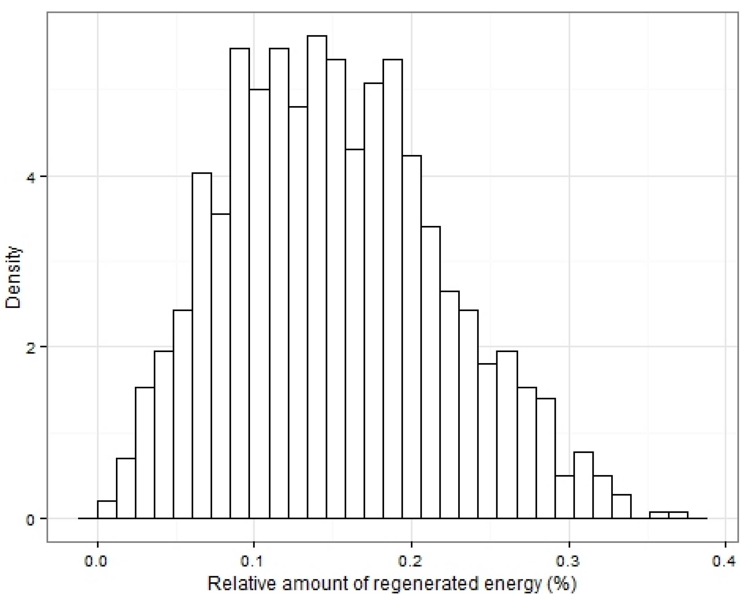
Figure 12 depicts the distribution of the relative amount of regenerated energy, defined as the ratio of the total amount of energy returned to the battery to the total amount of energy extracted from the battery. Figure 12 shows that while the average percentage of regenerated energy is about 15%, regenerated percentages can go up to 40% in extreme cases.
Figure 12. Distribution of regenerated energy percentage for all trips.
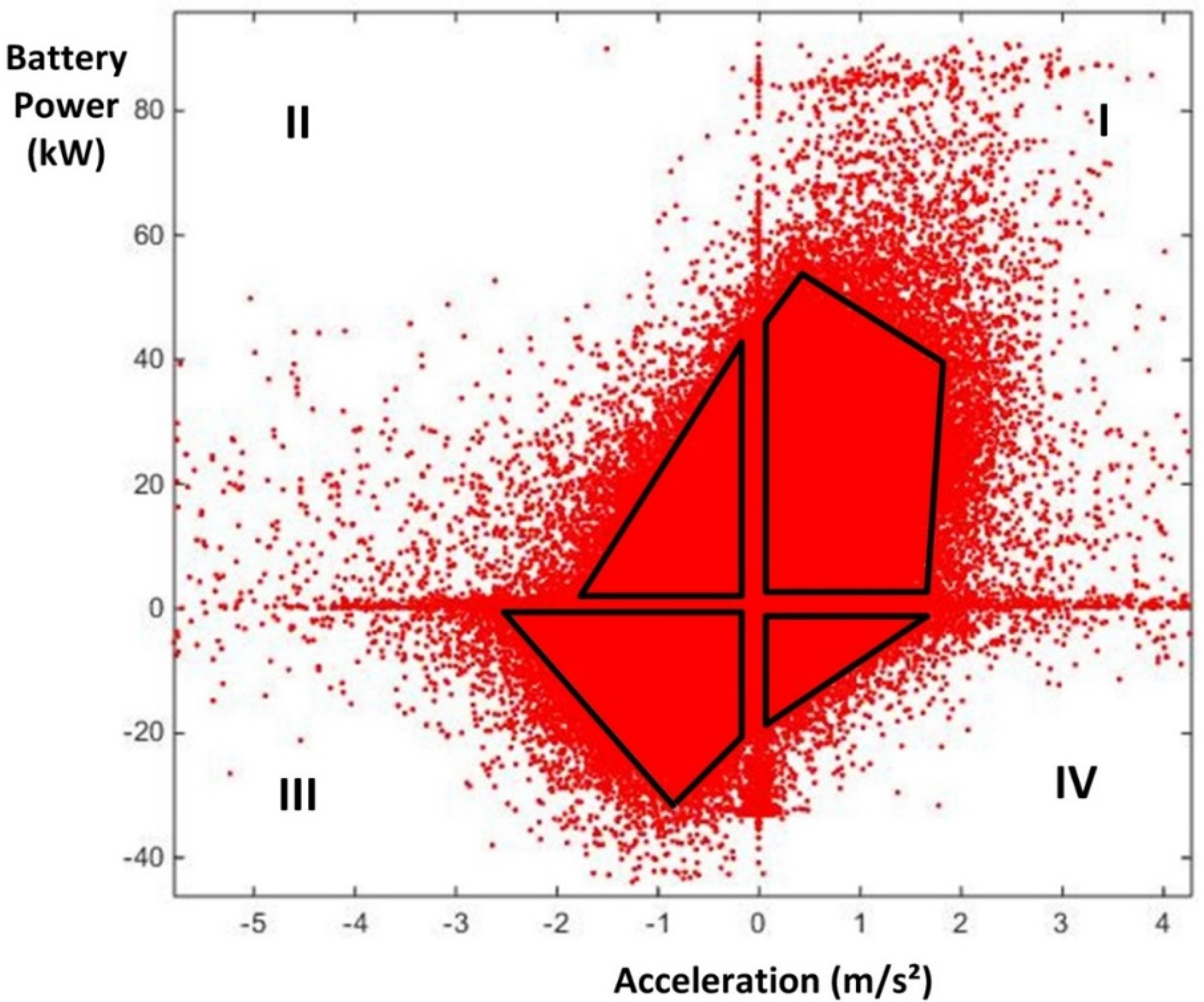
Energies 08 08573 g012
Figure 13. Four quadrant operation data points for the 2013 data.
Energies 08 08573 g013
The regenerative energy percentage is heavily dependent on the number of braking actions performed during a trip, which depends on road topology, traffic situation, and driving style, in combination with the regenerative braking strategy and drivetrain efficiency. This is shown in Mammosser et al. [17], where efficiency maps for regenerative braking are generated as a function of the braking force and vehicle speed using a vehicle simulation tool. In the second and third models, part of the use of the vehicle (braking actions) is represented in the CMF+ and CMF, but these parameters do not include all effects. Regenerative braking only occurs within a torque and power window and driving style can have a further effect on efficient regenerative braking. Figure 13 depicts all the 2013 data points in an acceleration–battery power plane and illustrates the effect of driving style on regenerative braking. From Figure 13 it is observed that the regenerative power does not exceed 40 kW and has its largest value at a specific deceleration (at about −1 m/s2 here, but for more information on the accuracy of this value see Section 3 (Data Availability and Reliability)). This highlights the non-linear principle of the regenerative braking energy and should be thoroughly investigated to further improve the model.
The battery power-vehicle acceleration plane can be divided into four quadrants. Quadrant one consists of actions using traction power for acceleration (so positive battery power and acceleration) and quadrant three for regenerative braking (negative power and acceleration). Less obvious are the actions residing in quadrant 2 and 4. Quadrant 2 has use of traction power but decreasing speed (negative acceleration), meaning traction power is still being used but not sufficiently to overcome resistive forces (for example, slowing down while climbing a hill). Quadrant 4 consists of actions where there is positive acceleration yet power is regenerated. This seems a very artificial condition, but the easiest example of a situation that would allow that to happen is driving steeply downhill. For ease of view, the bulk of the data in each of these quadrants are marked with a black cross section. Figure 13 seems to have a great number of outliers or extreme values, but since more than 1 million data points are depicted, this is not abnormal. Although the arguments above show why further analysis is required to better model regenerative braking and driving style, the CMFs can be used to categorize the use of the vehicle and are important parameters in the linear regression models above.
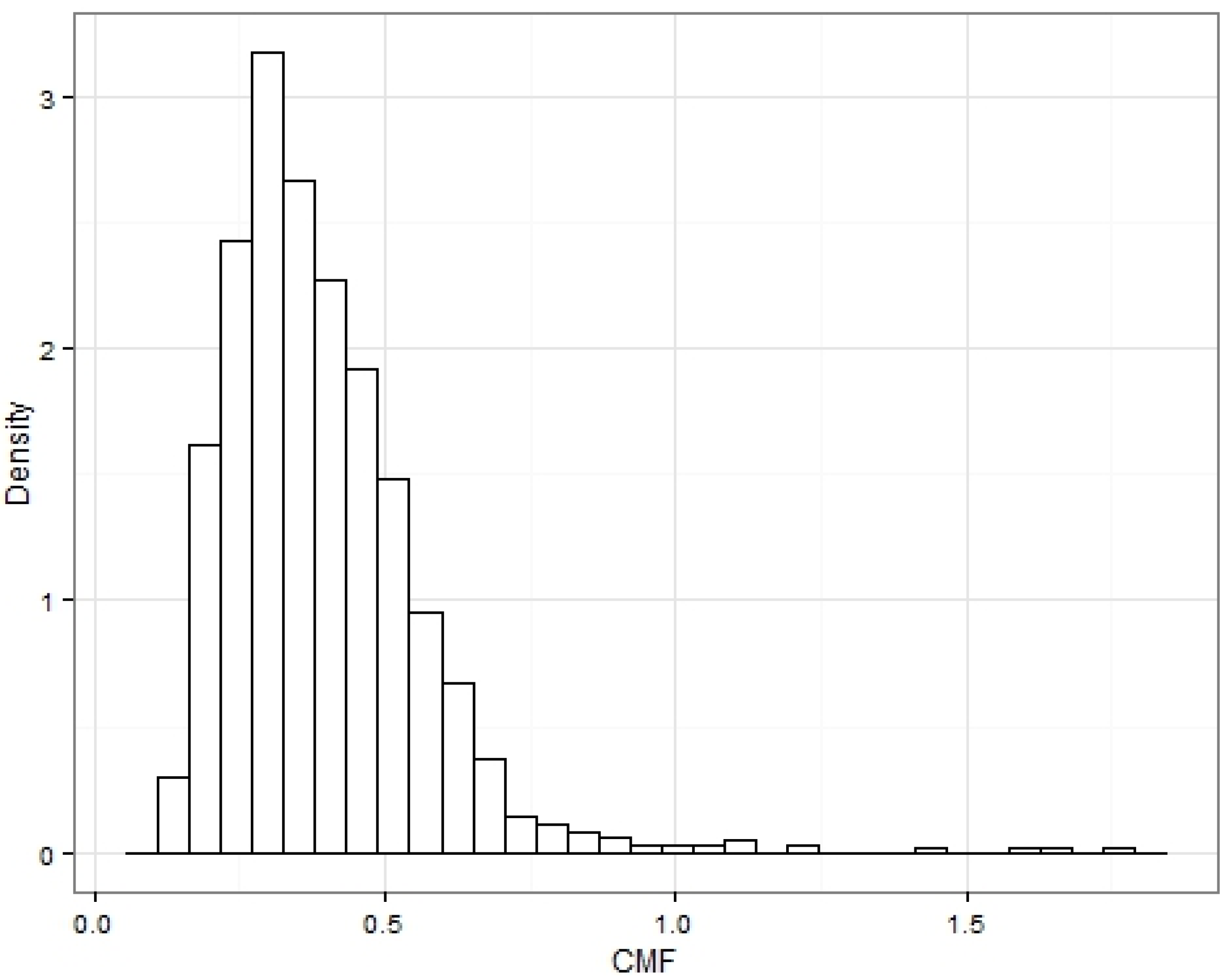
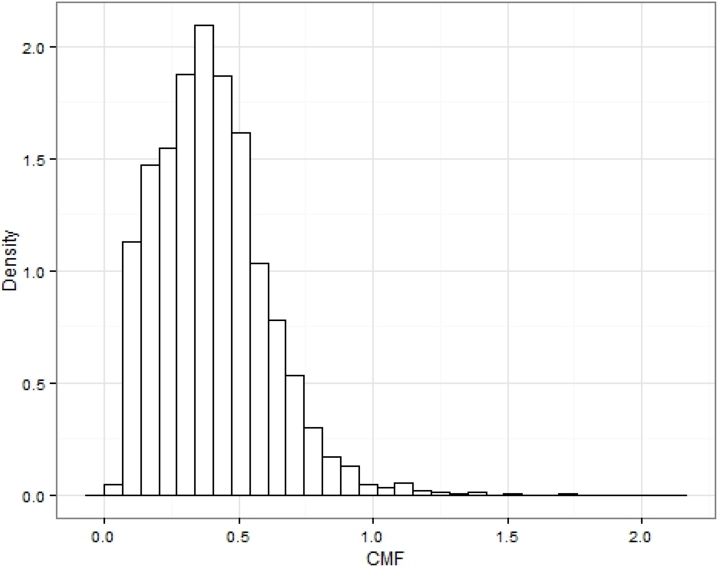
 Figure 14 and Figure 15 depict the distribution of the CMFs for macro-trips and micro-trips, respectively. Both show similar distributions and show that occurrences of CMFS greater than 1 are very rare and greater than 2 non-existent (macro trips did show CMFs greater than 2 but from statistical analysis these outliers were investigated and deleted from the sample because of the corrupted data). These CMFs are calculated from the speed in km/h and distance in km. Having a value varying between 0 and 1 is convenient for the characterization, as the CMF basically indicates the amount of kinetic energy change per km, which will vary according to the road topology/traffic situation and driving style.
Figure 14. Histogram of the constant motion factor for the macro trips.
Energies 08 08573 g014
Figure 15. Histogram of the constant motion factor for the micro-trips.
Energies 08 08573 g015
Another parameter influencing regenerative braking is the weight of the vehicle. Increased mass results in an increased kinetic energy per unit speed. Moreover, this can shift the regenerative braking window. To investigate the influence of increased mass on vehicle consumption, during a three-month test phase in 2015 the vehicle was loaded with 200 kg. We expected to see shifted regression coefficients for the acceleration and elevation terms, as well as increased average consumption. This was not, in fact, observed, but a longer monitoring period might be required for the energy consumption to be significantly different.

6. Conclusions

Using the underlying physical relationships expressed in the vehicle dynamics equation, three models for EV energy consumption prediction have been constructed by applying the statistical method of multiple linear regression to real-world trip and energy consumption data for an EV. Because the data set consists of one vehicle’s data only, the constructed models are drivetrain specific and potential differences in the impact of the external factors on real-world energy consumption for different EV types are not included in these models. Each model uses a different level of aggregation for the input parameters (predictors), which allows for prediction according to the available input data. One model uses kinematic parameters aggregated over trips; one model extended this model by including detailed acceleration parameters over the trip; and a third model uses detailed values of the kinematic parameters to predict the energy consumption over micro-trips. Multiple linear regression with a high correlation coefficient proved to be a good technique for predicting the energy consumption using aggregated trip data by accounting for a large portion of the variability residing in the data. Introducing more detailed trip data in the second model shifted the correlation coefficients and showed the importance of including a term representing the acceleration. From the results it is clear that moving towards a model with a higher level of detail has the potential to create a more accurate model. Both the first and second model had the concentration of the prediction errors within the 25% and stayed within that level for trips with energy consumption over a few kWhs. Using multiple linear regression on micro-trips in the third model resulted in regression coefficients that do not correspond to the underlying physical principles. Moreover, to make this model applicable, this detailed level of input has to be extracted and predicted from road, environmental, and traffic situations. Despite these drawbacks for the third model, in addition to a lower correlation coefficient and high constant term (so there is less variability accounted for), the prediction of the consumption over a complete trip had similar accuracy to the other two models, which indicates the potential of this method. So, further study of statistical outliers, mapping the non-linear effects of regenerative braking, and linking traffic situations and driving style with characteristic parameters such as the CMF have the potential to contribute to a model that is both accurate and extractable from available and statistical road data.

Acknowledgments

The authors would like to acknowledge the Agency for Innovation by Science and Technology in Flanders (IWT) as the funder for the PhD grant of Cedric De Cauwer, and Flanders Make for the support to our team. The authors would also like to acknowledge the EVA, iMOVE and EVTeclab platforms of the Flanders’ Living labs for providing the required framework to perform the research for this paper.

Author Contributions

Cedric De Cauwer contributed in all parts of the process of this publication: collecting the data, processing the data, constructing the model, statistical analysis, interpreting the results, and writing the paper. Joeri van Mierlo contributed in the construction of the model, the interpretation of the results, and reviewing the paper. Thierry Coosemans contributed in the construction of the model, the interpretation of the results, and reviewing the paper.

Conflicts of Interest

The authors declare no conflict of interest.

References

  1. Fotouhi, A.; Yusof, R.; Rahmani, R.; Mekhilef, S.; Shateri, N. A review on the applications of driving data and traffic information for vehicles’ energy conservation. Renew. Sustain. Energy Rev. 2014, 37, 822–833. [Google Scholar] [CrossRef]
  2. Wager, G.; McHenry, M.P.; Whale, J.; Bräunl, T. Testing energy efficiency and driving range of electric vehicles in relation to gear selection. Renew. Energy 2014, 62, 303–312. [Google Scholar] [CrossRef]
  3. Dib, W.; Chasse, A.; Moulin, P.; Sciarretta, A.; Corde, G. Optimal energy management for an electric vehicle in eco-driving applications. Control. Eng. Pract. 2014, 29, 299–307. [Google Scholar] [CrossRef]
  4. Shankar, R.; Marco, J. Method for estimating the energy consumption of electric vehicles and plug-in hybrid electric vehicles under real-world driving conditions. Intell. Transp. Syst. IET 2013, 7, 138–150. [Google Scholar] [CrossRef]
  5. Yao, E.; Yang, Z.; Song, Y.; Zuo, T. Comparison of electric vehicle’s energy consumption factors for different road types. Discret. Dyn. Nat. Soc. 2013, 2013, 328757:1–328757:7. [Google Scholar] [CrossRef]
  6. Badin, F.; le Berr, F.; Briki, H.; Petit, M.; Magand, S.; Condemine, E. Evaluation of EVs energy consumption influencing factors. In Proceedings of the 2013 World Electric Vehicle Symposium and Exhibition (EVS27), Barcelona, Spain, 17–20 November 2013; pp. 1–12.
  7. Kambly, K.R.; Bradley, T.H. Estimating the HVAC energy consumption of plug-in electric vehicles. J. Power Sources 2014, 259, 117–124. [Google Scholar] [CrossRef]
  8. Yuksel, T.; Michalek, J.J. Effects of Regional Temperature on Electric Vehicle Efficiency, Range, and Emissions in the United States. Environ. Sci. Technol. 2015, 49, 3974–3980. [Google Scholar] [CrossRef] [PubMed]
  9. Neaimeh, M.; Hill, G.A.; Hübner, Y.; Blythe, P.T. Routing systems to extend the driving range of electric vehicles. Intell. Transp. Syst. IET 2013, 7, 327–336. [Google Scholar] [CrossRef]
  10. Messagie, M.; Boureima, F.S.; Coosemans, T.; Macharis, C.; Van Mierlo, J. A range-based vehicle life cycle assessment incorporating variability in the environmental assessment of different vehicle technologies and fuels. Energies 2014, 7, 1467–1482. [Google Scholar] [CrossRef]
  11. Messagie, M.; Lebeau, K.; Coosemans, T.; Macharis, C.; van Mierlo, J. Environmental and financial evaluation of passenger vehicle technologies in Belgium. Sustainability 2013, 5, 5020–5033. [Google Scholar] [CrossRef]
  12. Nordelöf, A.; Messagie, M.; Tillman, A.M.; Söderman, M.L.; van Mierlo, J. Environmental impacts of hybrid, plug-in hybrid, and battery electric vehicles-what can we learn from life cycle assessment? Int. J. Life Cycle Assess. 2014, 19, 1866–1890. [Google Scholar] [CrossRef]
  13. de Cauwer, C.; Maarten, M.; Coosemans, T.; van Mierlo, J.; Heyvaert, S. Electric vehicle use and energy consumption based on real-world electric vehicle fleet trip and charge data and its impact on existing EV research models. In Proceedings of the International Electric Vehicle Symposium and Exhibition, Kintex, Korea, 3–6 May 2015; pp. 1–11.
  14. Lebeau, P.; de Cauwer, C.; van Mierlo, J.; Macharis, C.; Verbeke, W.; Coosemans, T. Conventional, hybrid, or electric vehicles: Which technology for an urban distribution centre? Sci. World J. 2015, 2015, 302867:1–302867:11. [Google Scholar] [CrossRef] [PubMed]
  15. Lohse-Busch, H. Advanced Powertrain Research Facility, Nissan Leaf Testing and Analysis; U.S. Department of Energy: Washington, DC, USA, 2012.
  16. Lv, C.; Zhang, J.; Li, Y.; Yuan, Y. Mechanism analysis and evaluation methodology of regenerative braking contribution to energy efficiency improvement of electrified vehicles. Energy Convers. Manag. 2015, 92, 469–482. [Google Scholar] [CrossRef]
  17. Mammosser, D.; Boisvert, M.; Micheau, P. Designing a set of efficient regenerative braking strategies with a performance index tool. Proc. Inst. Mech. Eng. Part D J. Automob. Eng. 2014, 228, 1505–1515. [Google Scholar] [CrossRef]
  18. Zou, Z.; Cao, J.; Cao, B.; Chen, W. Evaluation strategy of regenerative braking energy for supercapacitor vehicle. ISA Trans. 2014, 55, 234–240. [Google Scholar] [CrossRef] [PubMed]

