Torque Distribution Algorithm for an Independently Driven Electric Vehicle Using a Fuzzy Control Method

Abstract

The in-wheel electric vehicle is expected to be a popular next-generation vehicle because an in-wheel system can simplify the powertrain and improve driving performance. In addition, it also has an advantage in that it maximizes driving efficiency through independent torque control considering the motor efficiency. However, there is an instability problem if only the driving torque is controlled in consideration of only the motor efficiency. In this paper, integrated torque distribution strategies are proposed to overcome these problems. The control algorithm consists of various strategies for optimizing driving efficiency, satisfying driver demands, and considering tire slip and vehicle cornering. Fuzzy logic is used to determine the appropriate timing of intervention for each distribution strategy. A performance simulator for in-wheel electric vehicles was developed by using MATLAB/Simulink and CarSim to validate the control strategies. From simulation results under complex driving conditions, the proposed algorithm was verified to improve both the driving stability and fuel economy of the in-wheel vehicle.

1. Introduction

Eco-friendly vehicles are in the spotlight as a major research issue because of problems such as environmental pollution, energy, and resources. Hybrid electric vehicles (HEV) already take up a significant portion of the automobile market, and pure electric vehicles are also expected to advance into the automobile market with gradual progress of commercialization [1,2].

Most existing commercial electric vehicles are similar in structure to vehicles with internal combustion engines, and they generate torque on the left and right wheels using a motor and differential gear. When a vehicle is formed with such a structure, the batteries are loaded on the fuel tank or trunk, and the motor is positioned in place of the engine. However, since electric vehicles require an extremely large space for batteries and additional space for the attachment of electronic components like an inverter, unlike internal combustion engine vehicles, it is difficult to secure such space with the given structure [2,3].

An in-wheel system in which each wheel has a drive motor has been suggested to resolve this problem. The in-wheel system is at an advantage in terms of space because it simplifies the driving system, and the efficiency of the power system is increased as the power transmission components, such as the transmission and differential gear, are removed. Also, the Traction Control System (TCS) and Vehicle Dynamic Control System (VDC) can be enabled without an additional device because a motor that has faster response characteristics than the engine and hydraulic system is used for the operation and braking of each wheel. Accordingly, most existing studies of the in-wheel system have focused on improving the driving stability of vehicles, such as straight line driving performance, driving stability while cornering, turning performance through torque vectoring, and slip control on low-friction and asymmetric road surfaces [1,2,3,4,5,6,7,8,9,10,11].

Delay in commercialization of electric vehicles is not only caused by the problem of driving stability but also by short per-charge driving distance. However, studies on improving efficiency of in-wheel electric vehicles are still inadequate. Several recent studies presented driving strategies to improve efficiency of in-wheel electric vehicles. Gu et al. [12] proposed a method for optimizing the efficiency of in-wheel electric vehicles through conversion between two-wheel drive and four-wheel drive while taking into consideration the loss of motor and inverter. However, there are many problems involving maximizing the motor efficiency by only relying on two-wheel/four-wheel conversion. Lin et al. [13] developed a driving strategy for optimizing the driving torque where design of experiments (DOE) is used to extract the optimal driving torque ratio of the motor depending on the vehicle speed and the acceleration pedal. In addition, lower-layer sliding mode controller is proposed as a scheme for controlling the wheel slip rate. Chen et al. [14,15], while proposing various energy-efficient control allocation strategies, have studied to verify performance of each scheme in the diverse driving conditions. Wang et al. [16] presented a strategy for driving and braking force distribution that optimizes front and rear wheel efficiencies by considering the efficiency from the battery to the ground during driving and braking actions. Xu et al. [17] suggested a regenerative braking control strategy that optimizes efficiency and braking performance of EV by utilizing a fuzzy control strategy. Despite the foregoing, most of the existing literature has only put its focus on either driving or braking dynamics, whilst paying little attention on potential decrease in vehicular driving stability.

In this study, to improve efficiency of vehicles with in-wheel systems, a driving torque distribution strategy capable of positively controlling driving ratios of front wheels and rear wheels is presented. If design for increased efficiency is made with driving torque or braking torque concentrated on either front or rear wheels, a problem may occur causing driving stability to be lowered during rapid acceleration, cornering, or low-friction on-road driving. To solve such problem, a lower-layer controller is incorporated which judges the diverse driving condition to realize switching for driving force distribution. Its algorithm is configured so as to actively respond to offline driving conditions such as vehicle’s acceleration, cornering and tires’ slip ratios. In addition, a fuzzy control technique is utilized to prevent switching errors that may occur at the control intervention boundary of individual lower-layer controllers.

2. Performance Simulator for an Independent 4WD EV

The target of this study is a small electric vehicle that has four in-wheel motors for each wheel. Since there is no mechanical connection between the left and right wheels in the vehicle, the driving power is determined only by the control signal, so the vehicle might lose stability in some situations. Therefore, a control algorithm that enhances the driving stability must be developed during the development stage. However, the algorithm cannot be implemented or verified during the development stage because there is no actual vehicle. For this study, a simulation environment was built and the target system was modeled in order to analyze the driving performance of the target vehicle. The simulation environment provides methods to verify various algorithms before the vehicle is made, which can reduce the cost and time of development.

2.1. Battery Modelling

A battery is a device that stores electrical energy. In an electric vehicle, a battery gets energy by charging or from regenerative braking, and supplies electrical energy to the motors. An in-wheel electric vehicle repeats the charging and discharging process continuously, so the State of Charge (SOC) and the characteristics of charging have to be considered. The study uses the map of internal resistance to calculate the input/output power and SOC [11,18].

The voltage of the battery (U_a) during the charging and discharging process is calculated below according to Kirchhoff’s current law.

$$U_a=E-i_a{R}_i(\text{Discharge})$$

(1)

$$U_a=E+i_a{R}_i(\text{Charge})$$

(2)

where E is the electromotive force, R_i means the internal resistance of the battery, and i_a is the battery’s current load. The counter electromotive force and internal resistance are obtained from test results.

The power of the battery and the current in the charging and discharging stages can be calculated using the equations below.

$$P_{battery}=U_a\times i_a$$

(3)

$$U_a=\frac{P_{battery}}{i_a}=E-i_a{R}_i$$

(4)

$$P_{battery}=E{i}_a-i_a^2{R}_i$$

(5)

$$i_a=\frac{E-\sqrt{E^2-4R_i{P}_{Battery\_required}}}{2R_i} (\text{Discharge})$$

(6)

$$i_a=\frac{-E+\sqrt{E^2+4R_i{P}_{Battery\_required}}}{2R_i} (\text{Charge})$$

(7)

where P_{Battery_required} is the power required for the battery. The output power from the battery (P_battery) is determined as shown below.

$$V=i_a\times R_i$$

(8)

$$P_{battery}=\text{V}\times i_a$$

(9)

where V is the output voltage of the battery. The SOC is closely related to the capacity of the battery. The remaining battery capacity can be calculated with the initial and used energy as shown below.

$$Q_u\left(i_a,t,\mathrm{\tau }\right)=Q_{\mathrm{\tau }}\left(\mathrm{\tau },i_a\right)-\underset{0}{\overset{t}{\int }}{i}_a\left(t\right)dt \underset{0}{\overset{t}{\int }}{i}_a\left(t\right)dt$$

(10)

where Q_u is the temporary usable capacity and Q_τ is the capacity of the accumulator. $\underset{0}{\overset{t}{\int }}{i}_a\left(t\right)dt$ is the used charge, and it can be obtained by integrating the current over time. This equation can be written as shown below with the maximum capacity of the battery, Q_τn.

$$Q_u\left(i_a,t,\mathrm{\tau }\right)=C_{\mathrm{\tau }}\left(\mathrm{\tau }\right){\eta }_A\left(i_a,\mathrm{\tau }\right)Q_{\mathrm{\tau }n}-\underset{0}{\overset{t}{\int }}{i}_a\left(t\right)dt$$

(11)

$$C_{\mathrm{\tau }}\left(\mathrm{\tau }\right)=\frac{Q_{\mathrm{\tau }}}{Q_{\mathrm{\tau }n}}{Q}_u,\hspace{0.17em}\hspace{0.17em}\hspace{0.17em}{\eta }_A\left(i_a,\mathrm{\tau }\right)={\left(i_a\frac{\left(t\right)}{I_n}\right)}^{-\mathrm{\beta }\left(\mathrm{\tau }\right)}$$

(12)

Finally, the current SOC is defined as the remaining battery capacity over the maximum capacity of the battery, and the equation is shown below.

$$\text{SOC}=\frac{Q_u}{Q_{\mathrm{\tau }n}}=\frac{C_{\mathrm{\tau }}\left(\mathrm{\tau }\right){\eta }_A\left(i_a,\mathrm{\tau }\right)Q_{\mathrm{\tau }n}-{\int }_0^t{i}_a\left(t\right)dt}{Q_{\mathrm{\tau }n}}$$

(13)

$$\text{SOC}=C_{\mathrm{\tau }}\left(\mathrm{\tau }\right){\eta }_A\left(i_a,\mathrm{\tau }\right)-\frac{1}{Q_{\mathrm{\tau }n}}\underset{0}{\overset{t}{\int }}{i}_a\left(t\right)dt$$

(14)

2.2. Motor Modeling

The target vehicle of this study has four in-wheel motors on each wheel. The in-wheel motors have a base rotational velocity of 2400 rpm with maximum torque of 59.7 Nm. Each motor has output power of 15 kW, which makes the vehicle’s output power 60 kW. The motors work as actuators when the vehicle is driven, and they work as generators when the vehicle velocity decreases.

The motor models get the angular velocity of each wheel from the vehicle model, the desired torque from the torque distribution model, and the regenerative braking torque from the brake model as inputs. Then the models calculate the output torque. The output torque (T_m) and angular velocity (ω_m) of the motor models are calculated as shown below [11,18].

The desired torque for the desired velocity is used as an input variable on the motor efficiency map. The motor efficiency map contains the efficiency of the motor at precise angular velocity and torque values. The experimental environment was created using a motor dynamo and a DC power supply, and the efficiency of the overall system was measured by comparing the input power with the output power passing through the inverter/motor. Linear interpolation was performed on the measured data to create an efficiency curve for the usage domain of the motor. Figure 1 shows the block diagram of the experimental environment and the actual experimental environment, and Figure 2 shows the efficiency characteristics of the system created for the experiment. The consumed power is calculated as shown below.

$$T_m=\frac{P_{m\_desired}}{{\omega }_m}$$

(15)

$${\omega }_m=\frac{V_{veh}\times N}{R_t}$$

(16)

$$P_{battery}=\frac{T_m\times {\omega }_m}{{\eta }_m}$$

(17)

where P_{m_desired} is the desired output power of the motor, V_veh is the velocity of the vehicle, N is the gear ratio of the final reduction gear, R_t is the radius of the tire, and η_m is the efficiency of the motor.

Figure 1. Experimental apparatus for measuring motor characteristics: (a) block diagram of the test bench for measuring motor characteristics; (b) photo of experimental apparatus.

Figure 1. Experimental apparatus for measuring motor characteristics: (a) block diagram of the test bench for measuring motor characteristics; (b) photo of experimental apparatus.

Figure 2. Motor efficiency characteristic curve.

Figure 2. Motor efficiency characteristic curve.

2.3. Vehicle Dynamics Modeling

A high degree of freedom (DOF) vehicle model is essential for estimating the stability of the vehicle in a vehicle dynamics simulation. A co-simulation environment has been built for the analysis of vehicle stability. Powertrain models on MATLAB/Simulink and CarSim, which is commercial software with 27 DOF, are used. Figure 3 displays the powertrain models on MATLAB/Simulink, and Figure 4 shows the co-simulation environment between CarSim and the powertrain models. Driving and braking torque, which is calculated in the powertrain model, is used as an input variable for the vehicle dynamics model. CarSim calculates the vehicle velocity, yaw rate, and angular velocity of each wheel with the driving and braking torque input and sends the output to the powertrain model. As mentioned, the vehicle performance simulator for a four-wheel independent driving vehicle is built, and the driving performance analysis and verification of the algorithm can be implemented [9].

Figure 3. Powertrain model using MATLAB/Simulink.

Figure 3. Powertrain model using MATLAB/Simulink.

Figure 4. Co-simulation with MATLAB/Simulink and CarSim.

Figure 4. Co-simulation with MATLAB/Simulink and CarSim.

A simulation was carried out to test the effectiveness of the vehicle dynamics model. Figure 5 shows experiment and Simulation under double lane change test condition. A double lane change test that can simultaneously test the velocity tracking and handling performance of the vehicle was performed among various vehicle performance tests. The velocity for the simulation and vehicle test was 60 km/h, and the angle of the steering wheel was selected as the input condition of the simulation. The results of the vehicle test and simulation are shown in Figure 6.

Figure 5. Comparison with experiment and simulation under double lane change test condition; (a) experiment; (b) simulation using CarSim.

Figure 5. Comparison with experiment and simulation under double lane change test condition; (a) experiment; (b) simulation using CarSim.

Figure 6. Comparison with experiment and simulation results under double lane change test condition: (a) roll angle; (b) lateral acceleration; (c) yaw rate.

Figure 6. Comparison with experiment and simulation results under double lane change test condition: (a) roll angle; (b) lateral acceleration; (c) yaw rate.

The vehicle driving test and simulation showed similar tendencies. The maximum values of the magnitude error and phase error were found for a quantitative comparison of the data. These data are presented in Table 1. Looking at the results, the maximum magnitude error of the roll angle was 11.4%, showing an accuracy of about 88.6%. The phase error was 4.8% with an accuracy of about 95.2%. In the case of lateral acceleration, the maximum magnitude error was 10.7%, showing an accuracy of about 89.3%. The phase error was 1.6% with an accuracy of about 98.4%. For the yaw rate, the maximum magnitude error was 11.4%, showing an accuracy of about 88.6%. The phase error was 4.8% with an accuracy of about 95.2%. The average magnitude error was about 7.93% and the average phase error was about 1.8%. Such errors indicate that a driving performance test based on a simulation can replace the actual vehicle test.

Table 1. Accuracy of simulation results compared with test results.

Vehicle data	Error [%]
	Magnitude	Phase
Roll angle	11.7	3.1
Lateral acceleration	10.7	1.6
Yaw rate	1.4	0.7
Average	7.93	1.8

Table 1. Accuracy of simulation results compared with test results.

Vehicle data	Error [%]
	Magnitude	Phase
Roll angle	11.7	3.1
Lateral acceleration	10.7	1.6
Yaw rate	1.4	0.7
Average	7.93	1.8

3. Torque Distribution Strategy Based on Fuzzy Logic

Since electric vehicles equipped with in-wheel motors allow for independent driving and braking of each wheel, the vehicle can be actively controlled through control of the driving/braking torque depending on the situation. Also, the efficiency of the vehicle can be increased by distributing the torque for each motor or selecting between two wheels and four wheels [13,14,15,16]. However, the stability of the vehicle can be greatly reduced by independent driving of the wheels if the driving/braking torque cannot be stably controlled during acceleration or braking. In order to resolve this problem, this study proposes a control strategy to judge different driving situations using Fuzzy logic and to differentiate the distribution of the torque.

3.1. Torque Distribution Strategy for Optimizing Driving Efficiency

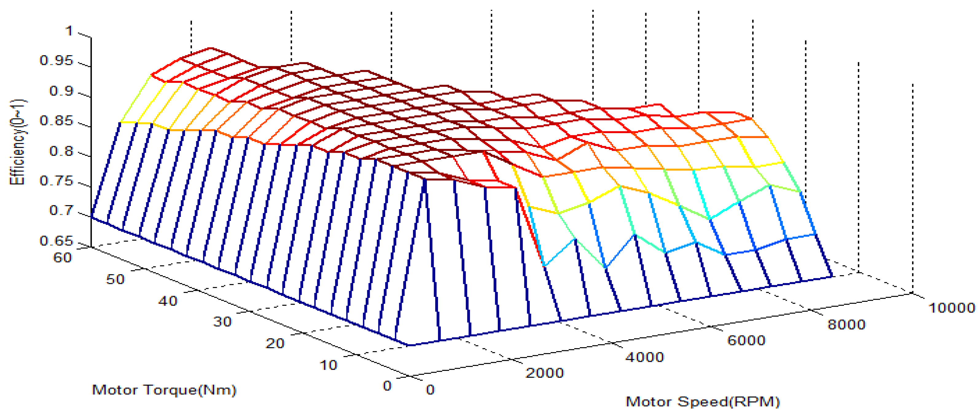
Vehicles attached with four in-wheel motors can drive each motor with independent torque, and the total torque wanted by the driver can be distributed at different ratios. This advantage can be used to increase the efficiency driving stability of the vehicle, as well as the efficiency. This study aims to present a control strategy that increases the efficiency by differentiating the ratio between the front and rear wheels and operating the driving torque output for efficient domain of the motor when the driver wants a certain driving torque. For instance, when a driver is expecting a total driving torque of 60 Nm, if the total driving efficiency of the motors are 85% when each motor has an output of 15 Nm and 90% when two motors have outputs of 20 Nm and the other two motors have outputs of 10 Nm, this method yields an efficient driving ratio. The efficiency characteristics of the overall system must first be understood in order to create such an algorithm. In this study, an algorithm was formed to control the torque distribution ratio in the efficiency domain of actual motors using the efficiency characteristics of the motor-inverter system found through the experiment described in Section 2.2. The total driving/braking torque is calculated using the accelerator/brake pedal values of the driver and the velocity of the vehicle. 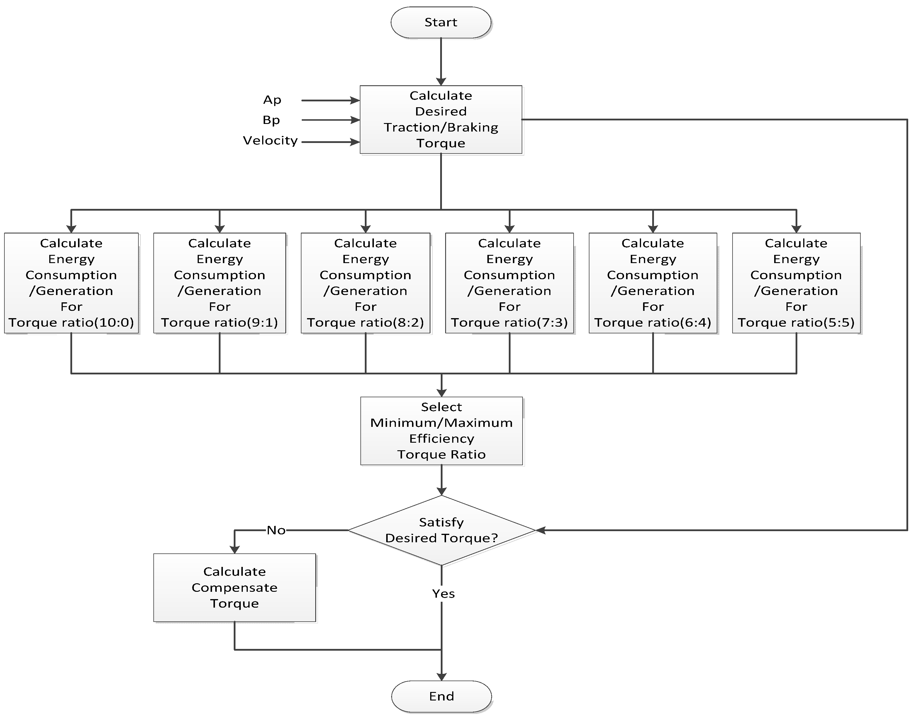The calculated total driving/braking torque and the efficiency curve of Figure 2 are used to estimate the actual power consumption according to the driving ratio. The control algorithm was prepared to increase the driving efficiency of the vehicle by selecting the driving ratio that consumes and regenerates optimum energy. Figure 7 shows the flow chart of the control algorithm.

Figure 7. Flow chart of the strategy for optimizing driving efficiency.

Figure 7. Flow chart of the strategy for optimizing driving efficiency.

3.2. Torque Distribution Strategy Considering Driver’s Acceleration Demand

If a driving torque distribution strategy is developed by considering a vehicle’s efficiency only, there may occur such a problem as failing to meet the driver demanded torque for acceleration or causing driving stability to be decreased due to driving torque concentrated on the front or rear wheel when accelerated. Therefore, it is vital to develop a control strategy ensuring that the driver demand for acceleration or cruise driving is determined by using the driver’s accelerator pedal signals, thereby producing driving torque appropriate to such driver demand.

Information able to be made available to determine driver demand for acceleration includes the vehicle’s current velocity and the driver’s accelerator pedal position value (Ap). However, the simple use of these data values gives rise to difficulty in accurately determining the driver’s acceleration demand. For instance, the magnitude of the driver’s demand for acceleration may be big at lower speeds although signals are input with low pedal values; likewise, the magnitude of the driver’s demand for acceleration may be small at higher speeds although signals are input with comparatively high pedal values. Quantitative reference values are necessary to distinguish between acceleration and cruise modes according to the accelerator pedal value. To compute quantitative values, an evaluation index of the acceleration demand, α, is defined as follows.

$$\mathrm{\alpha }=\frac{VehicleVelocity}{AcceleratorPosition}$$

(18)

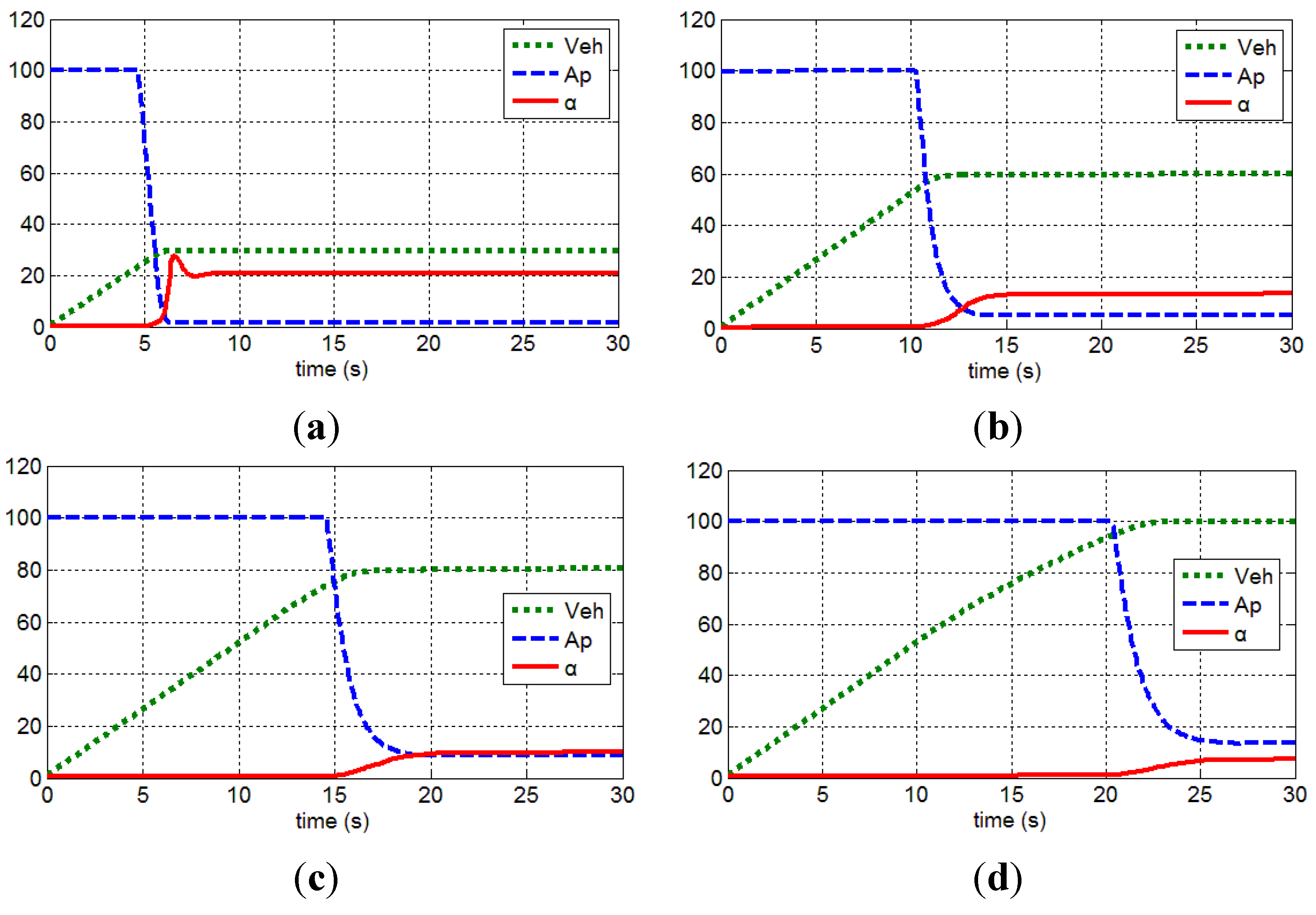
The term, α, in Equation (18) is defined as a value of the vehicle’s current velocity divided by the current Ap value, where the bigger the value α, the stronger the driver demand for cruising. At low vehicle speed, the input of even lower Ap value can be interpreted as having stronger demand for acceleration since the value α is relatively small, whereas at high speed of vehicle, the input of even higher AP value can be interpreted as having weaker demand for acceleration since the value α is relatively big. To investigate the range of the value α depending speeds in the cruise mode, a simple simulation was performed. The simulation pertains to assumptions of accelerating the vehicle from the stop position to 30 kph, 60 kph, 80 kph, and 100 kph for cruise drive. Figure 8 shows respective simulation speeds, Ap’s and α values, while Table 2 shows α values by simulation speed.

Resulting from the simulation, it can be known that values are overly small while accelerating, but α-values by speed remain constant when accelerated to specific speed and then cruised. Moreover, although the higher the cruising speed, the greater the AP values, it can be verified that the increased input value is small comparatively with the increased speed, resultantly causing the α-value to be lowered. Therefore, it is allowed to first set the reference α-values respectively matching the simulated speed levels, and then use them to judge as acceleration mode if the actual α-value is smaller than the reference value and as cruise mode if the actual α-value is equal to or bigger than the reference value. Nevertheless, as α-values during cruise mode vary with simulated speeds, reliance on α-values only makes it difficult to accurately determine whether the driver demand is for acceleration or for cruise driving. As a means to solve this problem, a fuzzy logic, as shown in Table 3, is presented to make the driver demand for acceleration verifiable by using the vehicle’s speed and α-values [19].

Figure 8. Variations of index α under various vehicle speed and accelerator position conditions; (a) 0–30 kph acceleration and cruise drive; (b) 0–60 kph acceleration and cruise drive; (c) 0–80 kph acceleration and cruise drive; (d) 0–100 kph acceleration and cruise drive.

Figure 8. Variations of index α under various vehicle speed and accelerator position conditions; (a) 0–30 kph acceleration and cruise drive; (b) 0–60 kph acceleration and cruise drive; (c) 0–80 kph acceleration and cruise drive; (d) 0–100 kph acceleration and cruise drive.

Table 2. Index α at different vehicle speeds.

Vehicle speed	α
30 kph	21
60 kph	13
80 kph	10
100 kph	8

Table 2. Index α at different vehicle speeds.

Vehicle speed	α
30 kph	21
60 kph	13
80 kph	10
100 kph	8

Table 3. Torque distribution strategy that reflects driver’s acceleration demand.

Fuzzy Controller Input Membership Function	Fuzzy Controller Rule Base
	1. If Velocity is 30 kph-range and alpha is Very-small then Torque-ratio is High-Acc;
	2. If Velocity is 30 kph-range and alpha is Small then Torque-ratio is High-Acc;
	3. If Velocity is 30 kph-range and alpha is Medium then Torque-ratio is Low-Acc;
	4. If Velocity is 30 kph-range and alpha is Large then Torque-ratio is Low-Acc;
	5. If Velocity is 30 kph-range and alpha is Very-large then Torque-ratio is Fixed;
	6. If Velocity is 60 kph-range and alpha is Very-small then Torque-ratio is High-Acc;
	7. If Velocity is 60 kph-range and alpha is Small then Torque-ratio is Low-Acc;
	8. If Velocity is 60 kph-range and alpha is Medium then Torque-ratio is Low-Acc;
	9. If Velocity is 60 kph-range and alpha is Large then Torque-ratio is Fixed;
	10. If Velocity is 80 kph-range and alpha is Very-small then Torque-ratio is High-Acc;
	11. If Velocity is 80 kph-range and alpha is Small then Torque-ratio is Low-Acc;
	12. If Velocity is 80 kph-range and alpha is Medium then Torque-ratio is Fixed;
	13. If Velocity is 100 kph-range and alpha is Very-small then Torque-ratio is High-Acc;
	14. If Velocity is 100 kph-range and alpha is Small then Torque-ratio is Low-Acc;
	15. If Velocity is 100 kph-range and alpha is Medium then Torque-ratio is Fixed.
Fuzzy Controller Output Membership Function	Fuzzy Control Surface

Table 3. Torque distribution strategy that reflects driver’s acceleration demand.

Fuzzy Controller Input Membership Function	Fuzzy Controller Rule Base
	1. If Velocity is 30 kph-range and alpha is Very-small then Torque-ratio is High-Acc;
	2. If Velocity is 30 kph-range and alpha is Small then Torque-ratio is High-Acc;
	3. If Velocity is 30 kph-range and alpha is Medium then Torque-ratio is Low-Acc;
	4. If Velocity is 30 kph-range and alpha is Large then Torque-ratio is Low-Acc;
	5. If Velocity is 30 kph-range and alpha is Very-large then Torque-ratio is Fixed;
	6. If Velocity is 60 kph-range and alpha is Very-small then Torque-ratio is High-Acc;
	7. If Velocity is 60 kph-range and alpha is Small then Torque-ratio is Low-Acc;
	8. If Velocity is 60 kph-range and alpha is Medium then Torque-ratio is Low-Acc;
	9. If Velocity is 60 kph-range and alpha is Large then Torque-ratio is Fixed;
	10. If Velocity is 80 kph-range and alpha is Very-small then Torque-ratio is High-Acc;
	11. If Velocity is 80 kph-range and alpha is Small then Torque-ratio is Low-Acc;
	12. If Velocity is 80 kph-range and alpha is Medium then Torque-ratio is Fixed;
	13. If Velocity is 100 kph-range and alpha is Very-small then Torque-ratio is High-Acc;
	14. If Velocity is 100 kph-range and alpha is Small then Torque-ratio is Low-Acc;
	15. If Velocity is 100 kph-range and alpha is Medium then Torque-ratio is Fixed.
Fuzzy Controller Output Membership Function	Fuzzy Control Surface

A rule-based control is configured by using input membership functions, i.e., vehicle speed and α-values to determine driver demand for acceleration. The output membership function outputs torque ratio between 1 and 0, where values closer to 1 are judged closer to the cruise driving condition, thereby producing driving torque for which an efficiency-optimized torque distribution strategy is applied, while values closer to 0 are judged closer to the acceleration driving condition, thereby producing driving torque in which torque is distributed 5:5 to the front and rear wheels.

3.3. Torque Distribution Strategy Considering Tire Slip

When the vehicle is driving, slip occurs between the tires of the vehicle and the road surface. Here, the friction coefficient differs according to the amount of slip between the tires and the road surface. The torque delivered from the wheels is determined based on the friction coefficient. Therefore, when the torque that needs to be distributed into four wheels is excessively concentrated on the front or rear wheels, the slip ratio can increase rapidly. If the vehicle velocity is V and the velocity of each wheel is V_ω, the slip ratio, λ, is defined as shown below.

$$\lambda =\frac{V_{\omega }-V}{\max (V_{\omega },V)}$$

(19)

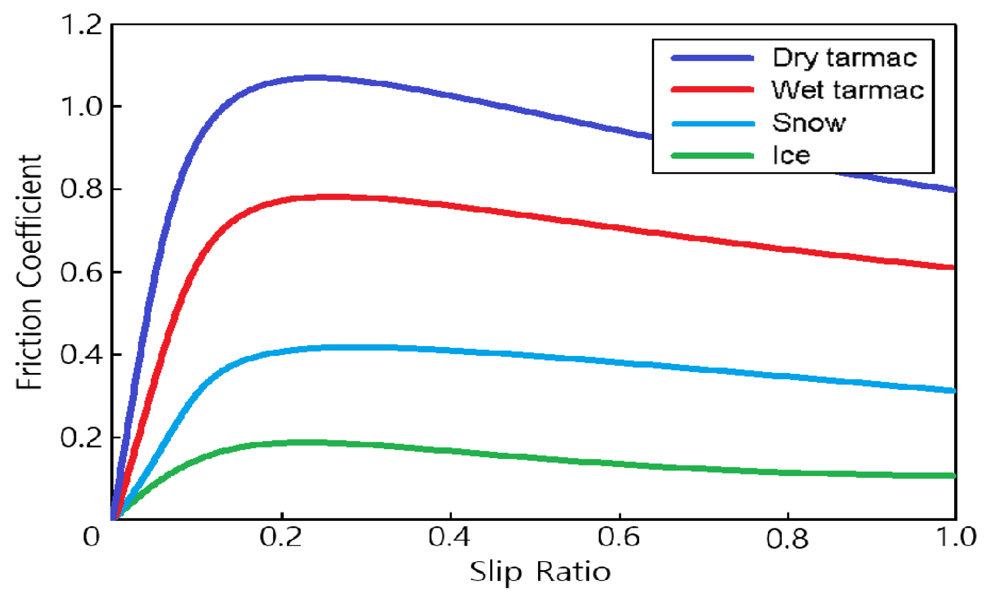
The friction coefficient between tires and the road surface has a general trend of increasing proportionally until a slip ratio of 0.2, reaching a maximum friction coefficient near 0.2, and rapidly decreasing after the maximum. Figure 9 is a graph that shows the rough relationship between the slip ratio and the friction coefficient [20]. Therefore, the slip controller generally controls the slip ratio so that it is maintained near 0.2. However, as mentioned earlier, this paper determines how to distribute the given total torque into each wheel prior to the intervention of the slip controller instead of maintaining the slip ratio through active control of the torque. Instability of the vehicle can be increased by controlling the slip ratio to 0.18–0.2, which is similar to an ordinary slip controller. For more active control intervention, a slip domain of about 0.08–0.12 was selected as the transient section, and a slip section of about 0.15 was selected as the unstable domain. The output membership function was configured to an output torque ratio between 1 and 0 as in the torque distribution strategy that reflects the will of the driver. Table 4 shows the developed Fuzzy logic.

Figure 9. Relationship between slip ratio and friction coefficient.

Figure 9. Relationship between slip ratio and friction coefficient.

Table 4. Torque distribution strategy considering tire slip.

Fuzzy Controller Input Membership Function	Fuzzy Controller Rule Base
	1. If Slip-Ratio is Stable and Slip-Ratio-differential is Small then Torque-ratio is Stable;
	2. If Slip-Ratio is Stable and Slip-Ratio-differential is Medium then Torque-ratio is Stable;
	3. If Slip-Ratio is Stable and Slip-Ratio-differential is Large then Torque-ratio is Transient;
	4. If Slip-Ratio is Transient and Slip-Ratio-differential is Small then Torque-ratio is Stable;
	5. If Slip-Ratio is Transient and Slip-Ratio-differential is Medium then Torque-ratio is Transient;
	6. If Slip-Ratio is Transient and Slip-Ratio-differential is Large then Torque-ratio is Unstable;
	7. If Slip-Ratio is Unstable and Slip-Ratio-differential is Small then Torque-ratio is Unstable;
	8. If Slip-Ratio is Unstable and Slip-Ratio-differential is Medium then Torque-ratio is Unstable;
	9. If Slip-Ratio is Unstable and Slip-Ratio-differential is Large then Torque-ratio is Unstable.
Fuzzy Controller Output Membership Function	Fuzzy Control Surface

Table 4. Torque distribution strategy considering tire slip.

Fuzzy Controller Input Membership Function	Fuzzy Controller Rule Base
	1. If Slip-Ratio is Stable and Slip-Ratio-differential is Small then Torque-ratio is Stable;
	2. If Slip-Ratio is Stable and Slip-Ratio-differential is Medium then Torque-ratio is Stable;
	3. If Slip-Ratio is Stable and Slip-Ratio-differential is Large then Torque-ratio is Transient;
	4. If Slip-Ratio is Transient and Slip-Ratio-differential is Small then Torque-ratio is Stable;
	5. If Slip-Ratio is Transient and Slip-Ratio-differential is Medium then Torque-ratio is Transient;
	6. If Slip-Ratio is Transient and Slip-Ratio-differential is Large then Torque-ratio is Unstable;
	7. If Slip-Ratio is Unstable and Slip-Ratio-differential is Small then Torque-ratio is Unstable;
	8. If Slip-Ratio is Unstable and Slip-Ratio-differential is Medium then Torque-ratio is Unstable;
	9. If Slip-Ratio is Unstable and Slip-Ratio-differential is Large then Torque-ratio is Unstable.
Fuzzy Controller Output Membership Function	Fuzzy Control Surface

3.4. Torque Distribution Strategy Considering Vehicle Cornering

When the vehicle turns, the rotational speed of each wheel is affected by the difference in the turning radius between the inner wheel and outer wheel. Thus, in the case of vehicles with a general driving mechanism that delivers torque to each wheel using a single driving source, it is essential to attach a differential gear to deliver torque while overcoming the difference in wheel speed between the inner and outer wheels of the vehicle when cornering. Differential gear is also used by the recent AWD (All-Wheel Drive) method. A difference in turning radius not only occurs between the inner and outer wheels, but also between the front and rear wheels. Even if there is a difference in rotational speed between the propeller shaft that drives the rear wheels and the propeller shaft that drives the front wheels upon cornering of the vehicle, the difference between the front and rear wheels can be compensated through application of the differential gear. This allows for soft cornering at high velocity. However for independently driven vehicles, the differential gear is removed and the turning performance can be reduced because the power source independently drives each wheel. This study proposes a control algorithm for a virtual electronic differential gear to resolve such a problem.

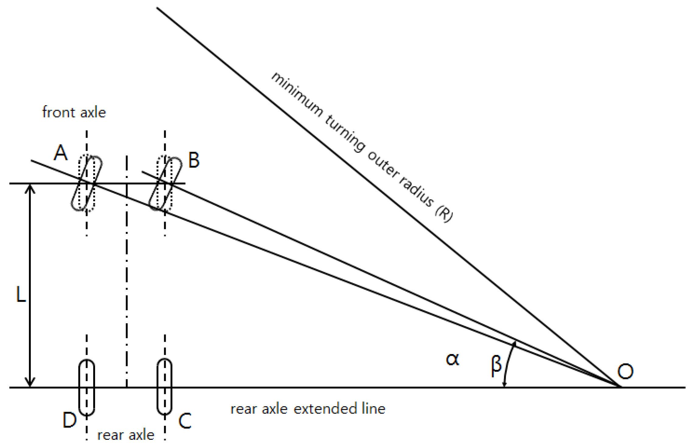
When the vehicle turns, a difference in turning radius is generated between the inner and outer wheels. A difference in turning radius between the front and rear wheels is generated as well. As shown in Figure 10, the turning radius ($\overline{OA}$) of the outer front wheel(A) is largest, and is therefore defined as the representative turning radius(R) of the vehicle.

In Figure 10, the turning radius of each wheel can be found by drawing a central extension line for each wheel from the central point O of the turning radius. The lines for the inner rear wheel(C) and outer rear wheel (D) can be assumed as $\overline{OC}$ and $\overline{OD}$, respectively. For the front wheels, a triangle is formed with the central point O by drawing an extension line with a length that is identical to the wheel space(L) from each rear wheel. According to the Pythagorean Theorem, the turning radius $\overline{OA}$ of the outer front wheel (A) and the turning radius $\overline{OB}$ of the inner front wheel(B) are as follows.

$$\overline{OA}=\sqrt{{\overline{OD}}^2+L^2}$$

(20)

$$\overline{OB}=\sqrt{{\overline{OC}}^2+L^2}$$

(21)

Figure 10. Turning radius of each wheel.

Figure 10. Turning radius of each wheel.

The turning radius of the vehicle can be estimated as shown below using the steering angle(δ) and yaw rate (γ) [21].

$$R=\frac{L}{\delta }(\text{Low speed})$$

(22)

$$R=\frac{v}{\gamma }(\text{High speed})$$

(23)

The estimated turning radius(R) uses the center of the rear wheel axle on the rear axle as the reference. When the wheel tread of the vehicle is defined as t, the turning radius of each wheel is as follows.

$$R_{FL}=\sqrt{{(R+\frac{t}{2})}^2+L^2}$$

(24)

$$R_{FR}=\sqrt{{(R-\frac{t}{2})}^2+L^2}$$

(25)

$$R_{RL}=R+\frac{t}{2}$$

(26)

$$R_{RR}=R-\frac{t}{2}$$

(27)

The angular velocity of the vehicle is calculated using the vehicle velocity and turning radius as shown below.

$${\omega }_{veh}=\frac{V_{veh}}{R}$$

(28)

Ultimately, the wheel velocity of each wheel can be expressed as follows using the angular velocity of the vehicle.

$$V_{FL}=R_{FL}{\omega }_{veh}$$

(29)

$$V_{FR}=R_{FR}{\omega }_{veh}$$

(30)

$$V_{RR}=R_{RR}{\omega }_{veh}$$

(31)

$$V_{RL}=R_{RL}{\omega }_{veh}$$

(32)

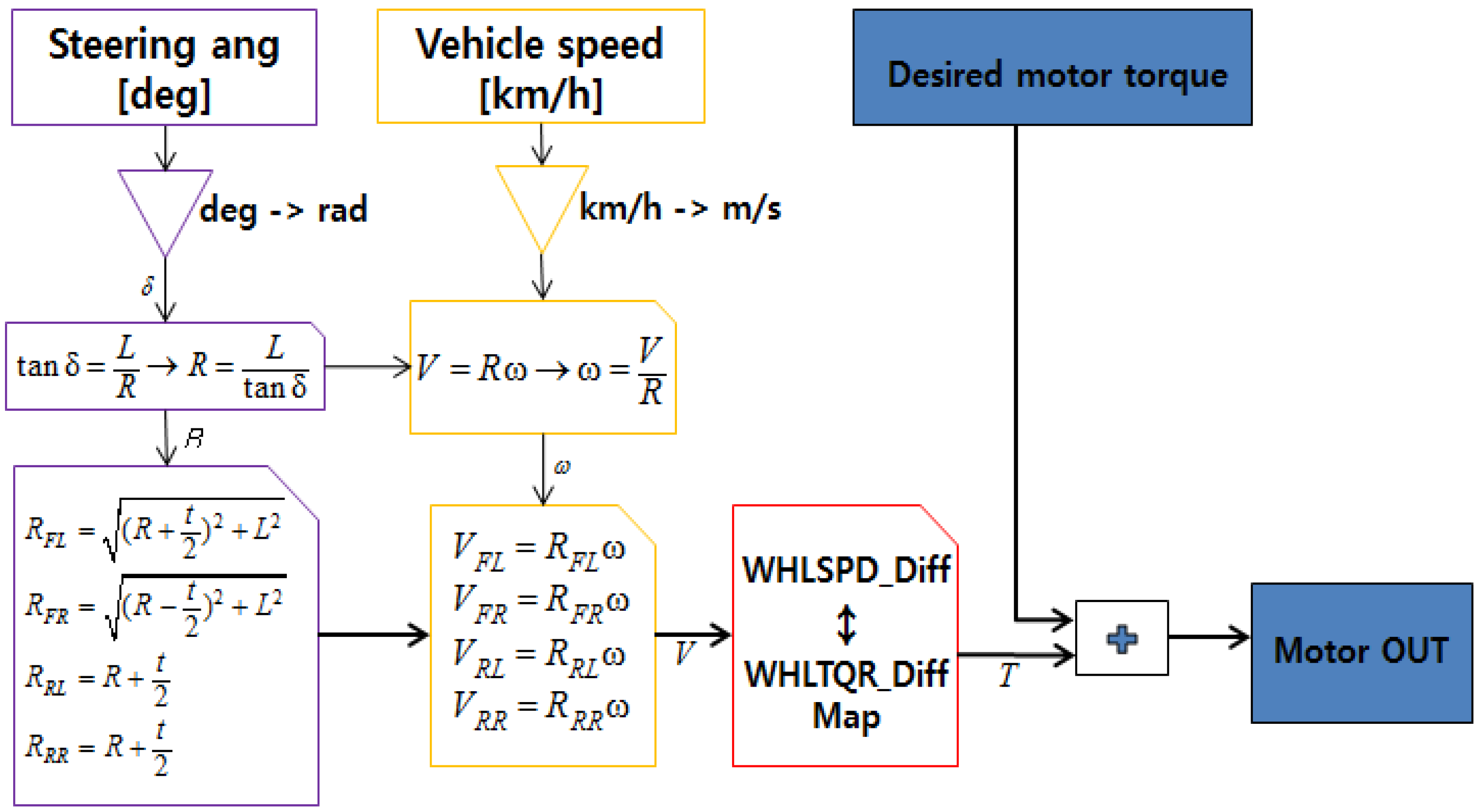
In order to track the velocity of each wheel calculated as shown above, the control logic shown in Figure 11 was created to output a different driving torque for each wheel. The wheel velocity-torque relationship was converted into a map through experimentation to apply the control algorithm to a vehicle, and the reliability of the algorithm was increased by applying the map to the actual control algorithm.

Figure 11. Control concept of electric differential gear.

Figure 11. Control concept of electric differential gear.

The torque distribution strategy based on Fuzzy logic was formed using the steering value of the driver and the vehicle velocity to determine the application of driving torque found using the control logic to the vehicle. Table 5 shows the torque distribution strategy considering a cornering situation. Like the two distribution strategies presented earlier, the driving torque delivered by an efficient distribution strategy is output as the output value is closer to 1, and a driving torque that reflects a cornering situation is output as the output value is closer to 0.

Table 5. Torque distribution strategy considering vehicle cornering.

Fuzzy Controller Input Membership Function	Fuzzy Controller Rule Base
	1. If VehSpeed is LowSpeed and STRAng is LowSTR then TorqueRatio is StableSTR;
	2. If VehSpeed is LowSpeed and STRAng is MidSTR then TorqueRatio is StableSTR;
	3. If VehSpeed is LowSpeed and STRAng is HighSTR then TorqueRatio is TransientSTR;
	4. If VehSpeed is MidSpeed and STRAng is LowSTR then TorqueRatio is StableSTR;
	5. If VehSpeed is MidSpeed and STRAng is MidSTR then TorqueRatio is TransientSTR;
	6. If VehSpeed is MidSpeed and STRAng is HighSTR then TorqueRatio is UnstableSTR;
	7. If VehSpeed is HighSpeed and STRAng is LowSTR then TorqueRatio is TransientSTR;
	8. If VehSpeed is HighSpeed and STRAng is MidSTR then TorqueRatio is UnstableSTR;
	9. If VehSpeed is HighSpeed and STRAng is HighSTR then TorqueRatio is UnstableSTR.
Fuzzy Controller Output Membership Function	Fuzzy Control Surface

Table 5. Torque distribution strategy considering vehicle cornering.

Fuzzy Controller Input Membership Function	Fuzzy Controller Rule Base
	1. If VehSpeed is LowSpeed and STRAng is LowSTR then TorqueRatio is StableSTR;
	2. If VehSpeed is LowSpeed and STRAng is MidSTR then TorqueRatio is StableSTR;
	3. If VehSpeed is LowSpeed and STRAng is HighSTR then TorqueRatio is TransientSTR;
	4. If VehSpeed is MidSpeed and STRAng is LowSTR then TorqueRatio is StableSTR;
	5. If VehSpeed is MidSpeed and STRAng is MidSTR then TorqueRatio is TransientSTR;
	6. If VehSpeed is MidSpeed and STRAng is HighSTR then TorqueRatio is UnstableSTR;
	7. If VehSpeed is HighSpeed and STRAng is LowSTR then TorqueRatio is TransientSTR;
	8. If VehSpeed is HighSpeed and STRAng is MidSTR then TorqueRatio is UnstableSTR;
	9. If VehSpeed is HighSpeed and STRAng is HighSTR then TorqueRatio is UnstableSTR.
Fuzzy Controller Output Membership Function	Fuzzy Control Surface

3.5. Integrated Algorithm for Torque Distribution

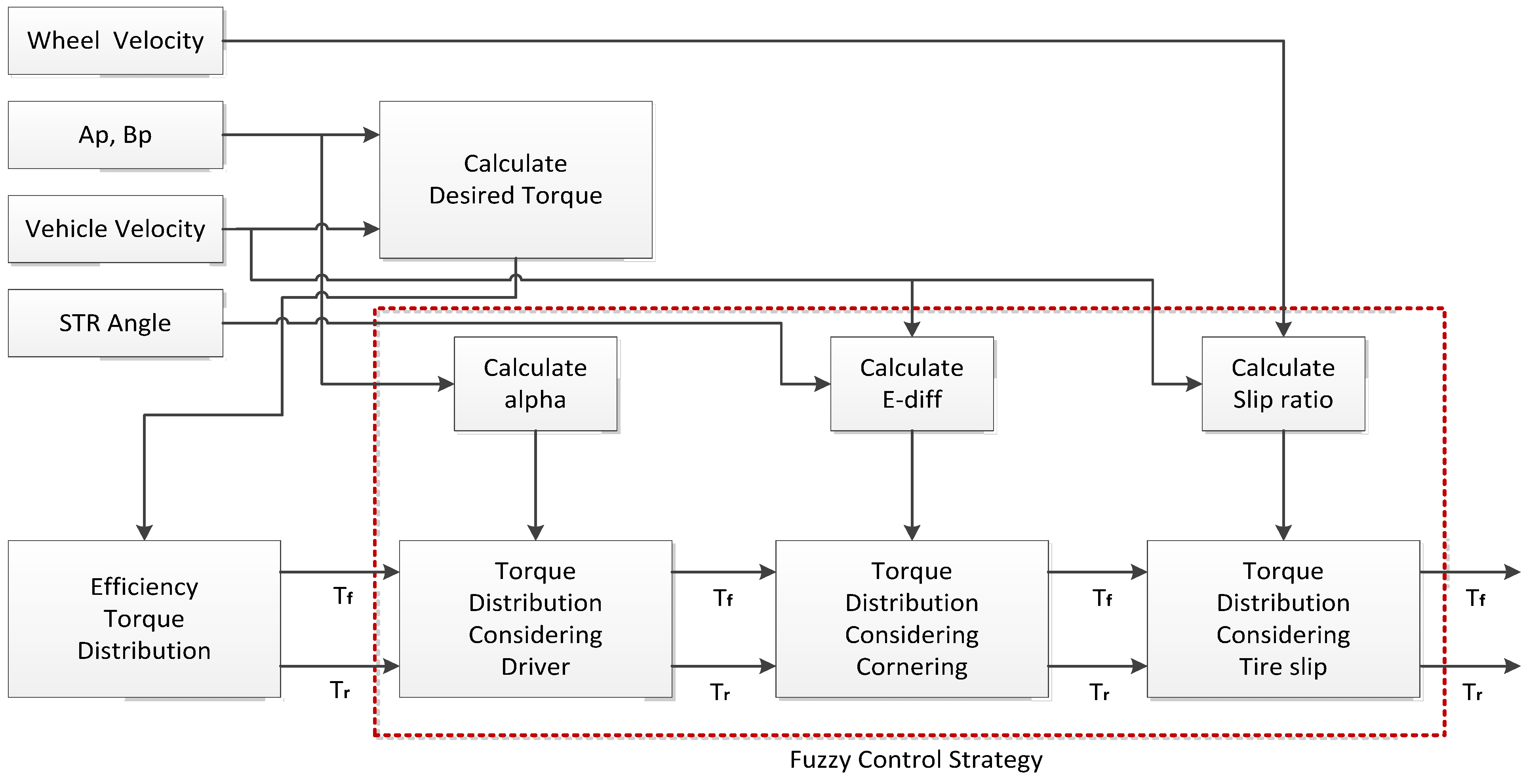
Torque distribution logic considering the efficiency of the driving system, torque distribution logic reflecting the acceleration will and braking will of the driver, and torque distribution logic considering the slip of the vehicle were developed. The effect of individual logic sets on the performance of the vehicle can differ according to how they are integrated. In this paper, each logic set was given a priority, and the distribution strategy with the highest priority was placed in the latter part so as to have greater impact on the final torque distribution. For example, since the energy efficiency algorithm determines the driving/braking torque without considering the stability of the vehicle, it was arranged to be the first algorithm to determine the torque, as it had the lowest importance in the final torque decision. Since slip of the vehicle is very likely to create unstable vehicle behavior, it was chosen to be the last algorithm such that it will have the greatest discretion. 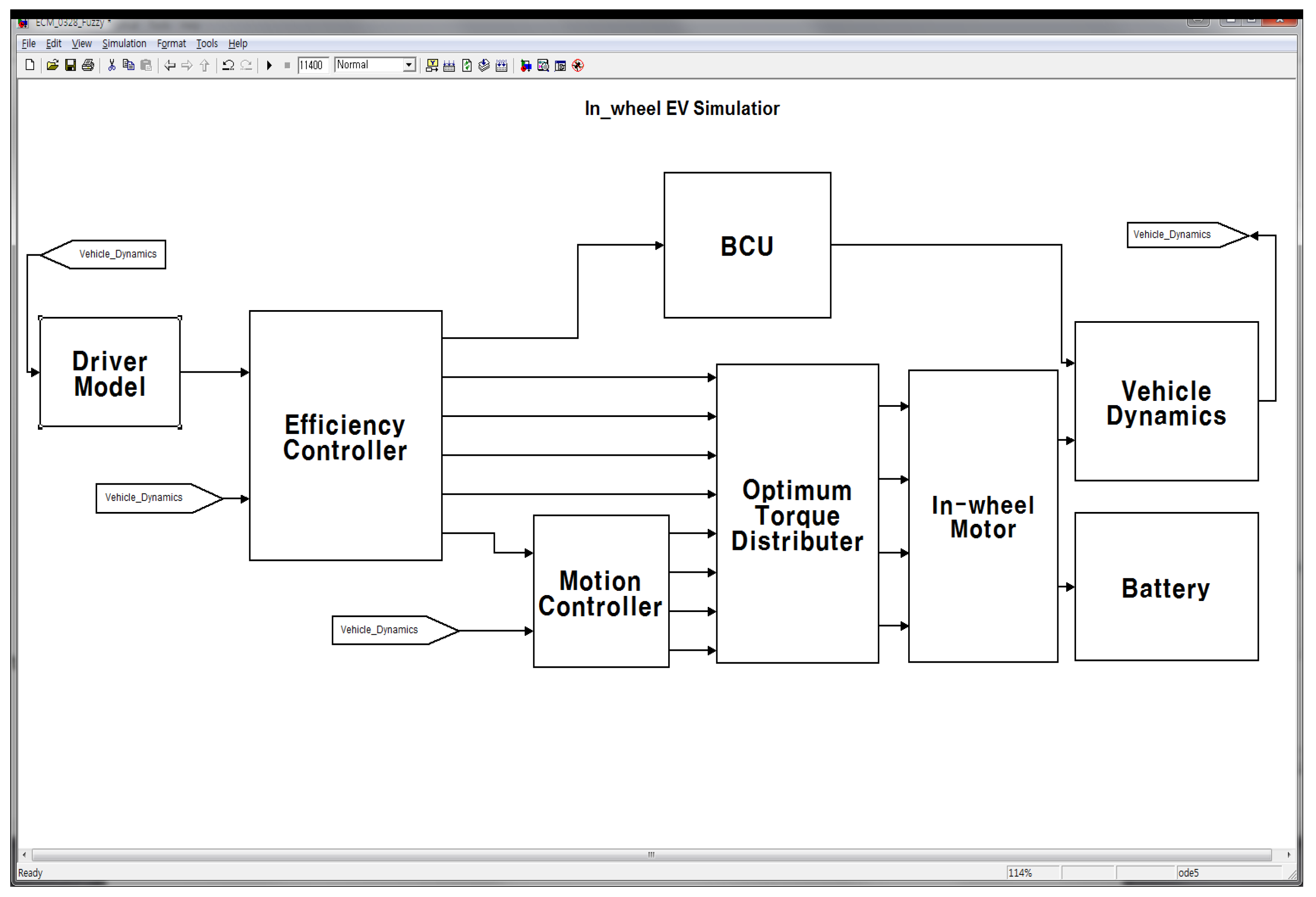Figure 12 shows a block diagram of the integrated algorithm. The priorities of the algorithms were arranged in the following order: efficiency distribution strategy, distribution strategy considering the driving will of the driver, distribution strategy considering cornering of the vehicle, and distribution strategy considering slip. The part indicated by red dotted lines reflects the Fuzzy control strategy.

Figure 12. Integrated torque distribution algorithm.

Figure 12. Integrated torque distribution algorithm.

4. Simulation and Discussion

4.1. Simulation Results for Analysis of Driving Stability

The torque distribution strategy for increasing efficiency was proposed in the previous chapter, and different torque distribution strategies were proposed to remove their effect on driving stability. A simulation was performed to find the effect of torque distribution strategies on driving stability. The first simulation condition was acceleration on a low friction road surface with a friction coefficient of 0.2. The driving results were compared for a vehicle that distributed torque into the front and rear wheels at a 5:5 ratio, a vehicle that applied the efficiency distribution strategy, and a vehicle that applied the integrated distribution strategy. The simulation results are shown in Figure 13. The maximum slip ratio of the vehicle that distributed torque into the front and rear wheels at a 5:5 ratio was below 0.1, and the acceleration of the vehicle was stable. On the contrary, the vehicle that applied the efficiency distribution strategy had excessive torque placed on the front wheels with a maximum slip ratio of about 0.65. This resulted in reduced acceleration performance. Increasing the slip of the vehicle increases the probability of spin, which can lead to fatal accidents. Lastly, the vehicle that applied the integrated torque distribution strategy placed greater torque on the front wheels in order to increase efficiency, but the slip of the vehicle was detected and the motor torque was controlled to maintain the maximum slip ratio at about 0.12 for stable acceleration performance. To quantitatively compare the three distribution strategies, the time taken to accelerate the vehicle to 60 km/h was indicated on the graph. The distribution strategy that maintained a 5:5 ratio had the fastest acceleration of 11.05 s. The vehicle that only applied the efficiency distribution strategy had its acceleration performance reduced by 11.3% to 12.3 s, whereas the performance of the vehicle that applied the integrated distribution strategy was only reduced by 0.45% to 11.1 s. Such results imply that differentiating the torque on the front and rear wheels through the integrated distribution strategy does not greatly reduce the driving stability.

Figure 13. Simulation results of the acceleration situation on a low friction road surface.

Figure 13. Simulation results of the acceleration situation on a low friction road surface.

The second simulation was carried out to examine the behavioral stability of the vehicle in a cornering situation. The conditions of the simulation are shown in Table 6.

Table 6. Simulation conditions in a cornering situation.

Driving condition	AP = 50%, μ = 0.85 Simulation time = 25 s
Steering gear ratio	16.58
Steering wheel angle	60

Table 6. Simulation conditions in a cornering situation.

Driving condition	AP = 50%, μ = 0.85 Simulation time = 25 s
Steering gear ratio	16.58
Steering wheel angle	60

Figure 14 shows the vehicle velocity and motor torque according to the torque distribution strategy. The velocity after 25 s in (b) decreases compared with the velocity in (a). It is considered that the fuel efficiency strategy decreases the stability of the vehicle as the vehicle velocity increases, whereas the velocity in (c) did not decrease in the high velocity region because the torque distribution strategy that considered cornering improved vehicle stability. This characteristic is shown as the torque after 20 s in (c). Figure 15 shows the vehicle trajectory where the vehicle with the fuel efficiency strategy has the largest turning radius. It is considered that the control algorithm for fuel efficiency distributes the torque mostly to the front wheels, and then the understeer occurs more than the other ones. However, the vehicle with the integrated control strategy has the smallest turning radius because the algorithm considers the cornering condition. Consequently, it is confirmed that the vehicle with the integrated control algorithm has a turning radius of 75.417 m, which is 2 m smaller than the 77.37 m turning radius of the vehicle with no control.

Figure 14. Simulation results of vehicle velocity and motor torque during circular drive: (a) fixed torque distribution; (b) applying distribution torque considering vehicle efficiency; (c) applying integrated torque distribution algorithm.

Figure 14. Simulation results of vehicle velocity and motor torque during circular drive: (a) fixed torque distribution; (b) applying distribution torque considering vehicle efficiency; (c) applying integrated torque distribution algorithm.

Figure 15. Trajectory of the simulation during circular driving.

Figure 15. Trajectory of the simulation during circular driving.

4.2. Simulation Results for Analysis of Driving Efficiency

A torque distribution algorithm for the front and rear wheels considering the efficiency of the motor was proposed to increase driving efficiency. A complex driving simulation used for the evaluation of fuel economy of internal combustion engine vehicles was performed to evaluate the validity of the algorithm. As for the conditions of the simulation, UDDS, NYCC, and JAPAN 10–15 were used. Figure 16 shows the simulation results of the UDDS condition. Figure 16a shows the velocity of the vehicle in UDDS driving mode from 0 to 200 s. The results indicate that there was no difference in the velocity traceability between the vehicle that applied the integrated torque control algorithm and the vehicle that applied the 5:5 torque distribution. Figure 16b,c shows the motor driving torque when the torque distribution strategy was applied or not applied. The driving torques of the front and rear wheels were always identical when the algorithm was not applied. When the integrated torque distribution strategy is applied, torque is simultaneously generated on the front and rear wheels in sections that require high acceleration such as the 20–30 s and 160–170 s domains to satisfy the driving will of the driver. Greater torque was placed on the front wheels with consideration of the motor efficiency in the 60–110 s domain when the vehicle was in cruise drive mode. Figure 16e,f depicts motor driving torques onto the motor efficiency map with and without the application of a torque distribution strategy, respectively, where the area inside the contour represents high efficiency area. For front-wheel motors, it can be seen that motor driving increases in the high efficiency area when the torque distribution strategy is applied, the tendency of which clearly differs with the case of regenerative braking. For rear-wheel motors, it can also be seen that the frequency of using low torque area during driving becomes lower in the range of low efficiency area that is between 2000–3000 RPM. However, the frequency of using low torque area during braking gets increased. This phenomenon is because the sum of the front-wheel efficiency and the rear-wheel efficiency is considered when distributing braking torque, which allows us to reasonably expect that the overall efficiency of vehicle is improved when even the efficiency improved due to braking torque is considered.

Figure 16. Simulation results in FTP-75 mode for 0–200 s: (a) vehicle velocity; (b) driving torque of each wheel with control; (c) driving torque of each wheel without control; (d) battery SOC with and without application of the control algorithm; (e) front motor operating point with motor efficiency map; (f) rear motor operating point with motor efficiency map.

Figure 16. Simulation results in FTP-75 mode for 0–200 s: (a) vehicle velocity; (b) driving torque of each wheel with control; (c) driving torque of each wheel without control; (d) battery SOC with and without application of the control algorithm; (e) front motor operating point with motor efficiency map; (f) rear motor operating point with motor efficiency map.

The per-charge driving distance was compared between diverse driving conditions to quantitatively evaluate the increase in efficiency caused by the algorithm. The simulation results are as shown in Table 7. The per-charge driving distance was improved by about 8.45% in FTP-75 mode, 8.09% in NYCC mode, and 7.21% in JAPANA 10-15 mode in vehicle driving efficiency simulation.

Table 7. Simulation results of efficiency testing at various driving cycles.

Driving Cycle	Driving Distance		Rate of Increment
	Without Control	With Control
FTP-75	93.5 km	101.4 km	8.45%
NYCC	60.5 km	65.4 km	8.09%
JAPAN 10–15	99.9 km	107.1 km	7.21%

Table 7. Simulation results of efficiency testing at various driving cycles.

Driving Cycle	Driving Distance		Rate of Increment
	Without Control	With Control
FTP-75	93.5 km	101.4 km	8.45%
NYCC	60.5 km	65.4 km	8.09%
JAPAN 10–15	99.9 km	107.1 km	7.21%

5. Conclusions

The simulation environment was constructed using MATLAB/Simulink and CarSim to evaluate the driving stability and fuel economy of electric vehicles with in-wheel motors.

A front and rear wheel torque distribution strategy was presented to drive a motor with optimum efficiency. Also, an integrated distribution strategy that accounts for various driving situations was proposed to prevent the efficiency distribution strategy from decreasing the driving will of the driver and the driving stability of the vehicle.

Different simulations were performed to test the proposed distribution strategies. First for the acceleration simulation on a low friction road surface, the vehicle with only the efficiency distribution strategy showed an 11.3% reduction in the acceleration performance, while the vehicle with the integrated distribution strategy showed an acceleration performance reduction of only about 0.45%. The simulation comparing normal cornering performance showed that the turning radius of the vehicle with the distribution strategy is about 2 m smaller than that of the vehicle without the distribution strategy. Lastly, the per-charge driving distance was improved by about 8.45% in FTP-75 mode, 8.09% in NYCC mode, and 7.21% in JAPAN 10–15 mode in vehicle driving efficiency simulation. The torque distribution strategies developed in this study were verified to increase the driving efficiency of vehicles while maintaining the driving stability of vehicles.