1. Introduction
For hygienic reasons, the minimum temperature of domestic hot water (DHW), in many countries, is within 55–60 °C [
1,
2,
3]. On the other hand, low temperature (LT) heat distribution systems are designed for the supply water temperature range of 35–40 °C. These different demands are challenging for the single-stage heat pump. The coefficient of performance (
COP value) decreases rapidly for high pressure ratios [
4].
For this reason, the heat pump is often used only for preheating and electric backup heaters are used to obtain DHW at 60 °C. This decreases energy performance. Ghoubali
et al. [
5] have found a 20%–25% decrease in the seasonal energy performance in a low-energy house.
The share of DHW in the total heat consumption has increased in new buildings due to the decreasing overall heat transfer coefficient (
U-value) of the building envelope and the increasing efficiency of exhaust air heat recovery systems. Even in single-family dwellings the energy for DHW heating is now of the same order of magnitude as the energy for space heating [
6]. The peak load of DHW is high and transient, and it is often higher than that of space heating [
7]. Therefore, a water tank is usually utilized as heat storage. A water tank is usually used also in space heating systems (buffer tank) for two reasons: firstly, to lengthen running periods of the compressor and secondly, due to different volume flow rates in the condenser and the heat distribution system. Thus, there are normally two water tanks in the ground source heat pump (GSHP) system: one LT tank acting as heat storage for the radiator or floor heating systems (heat storage tank HS1), and another high temperature (HT) tank for the DHW system (HS2). There is normally a DHW circulation system in apartment buildings to ensure that the temperature in the DHW pipe network remains high enough. For example, in Finland, the volume flow rate of the recirculation pump must be dimensioned so that the temperature of the return flow is >55 °C when the DHW supply temperature is between 58 °C and 65 °C [
1]. The heat effect of DHW circulation compensates heat losses of the DHW pipe network and drying towels.
Many studies are focused on improving the possibilities of the cycle, working fluids, or combining solar collectors or panels with a heat pump system [
6,
8,
9]. In the review paper, Ozgener and Hepbasli [
10] found three primary factors for influencing the energy performance of a GSHP system: the heat pump machine, the circulating pump or well pumps, and the ground coupling or ground water characteristics. In this study, a fourth factor is suggested: the space heating and DHW system. It is possible to improve energy performance in a simple way by utilizing water tanks for heating DHW in two stages and connecting two heat pumps in a series. This study points out that not only the temperature level but also the arrangement of the DHW system is important when trying to achieve high efficiency.
Three systems are often used in Finland:
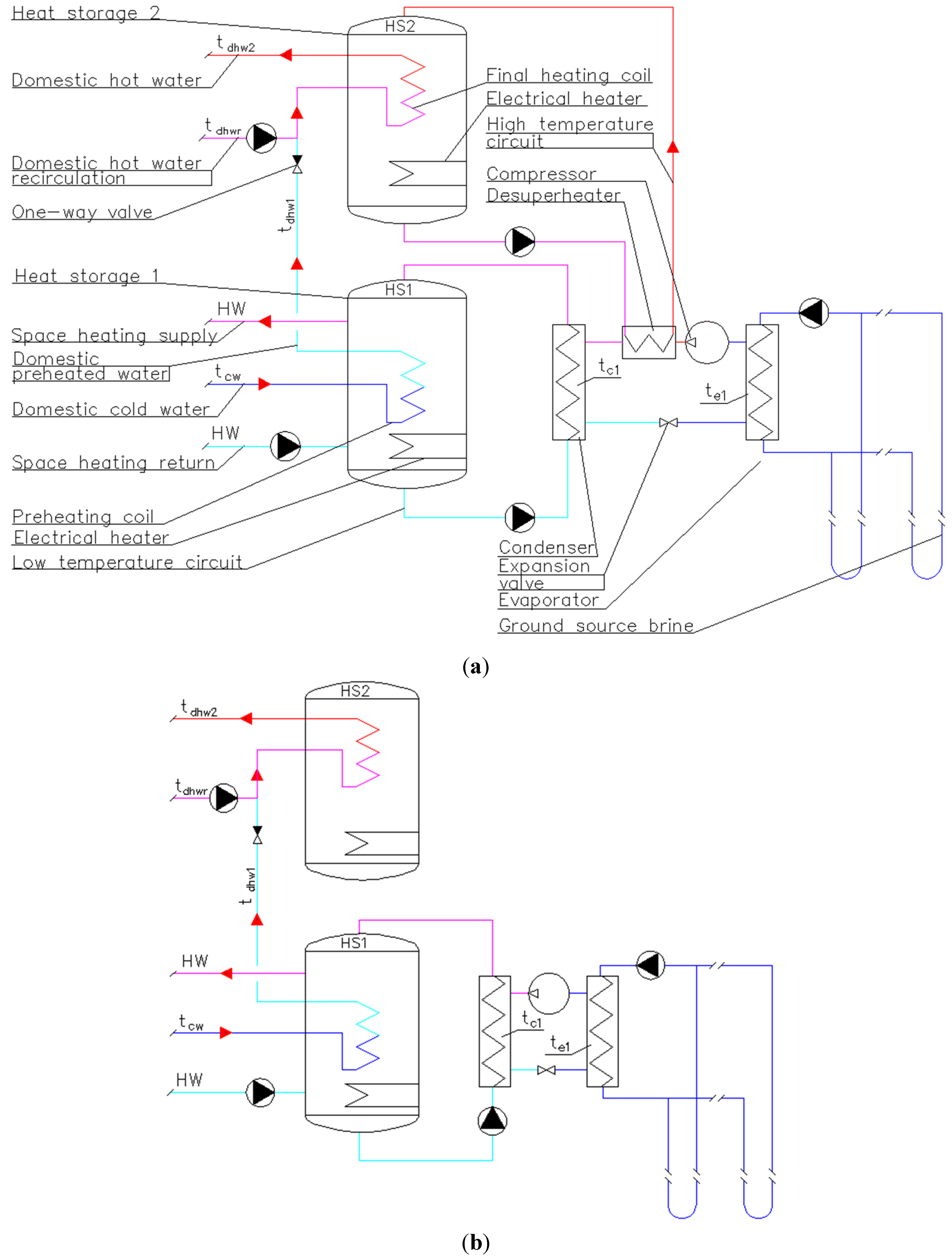
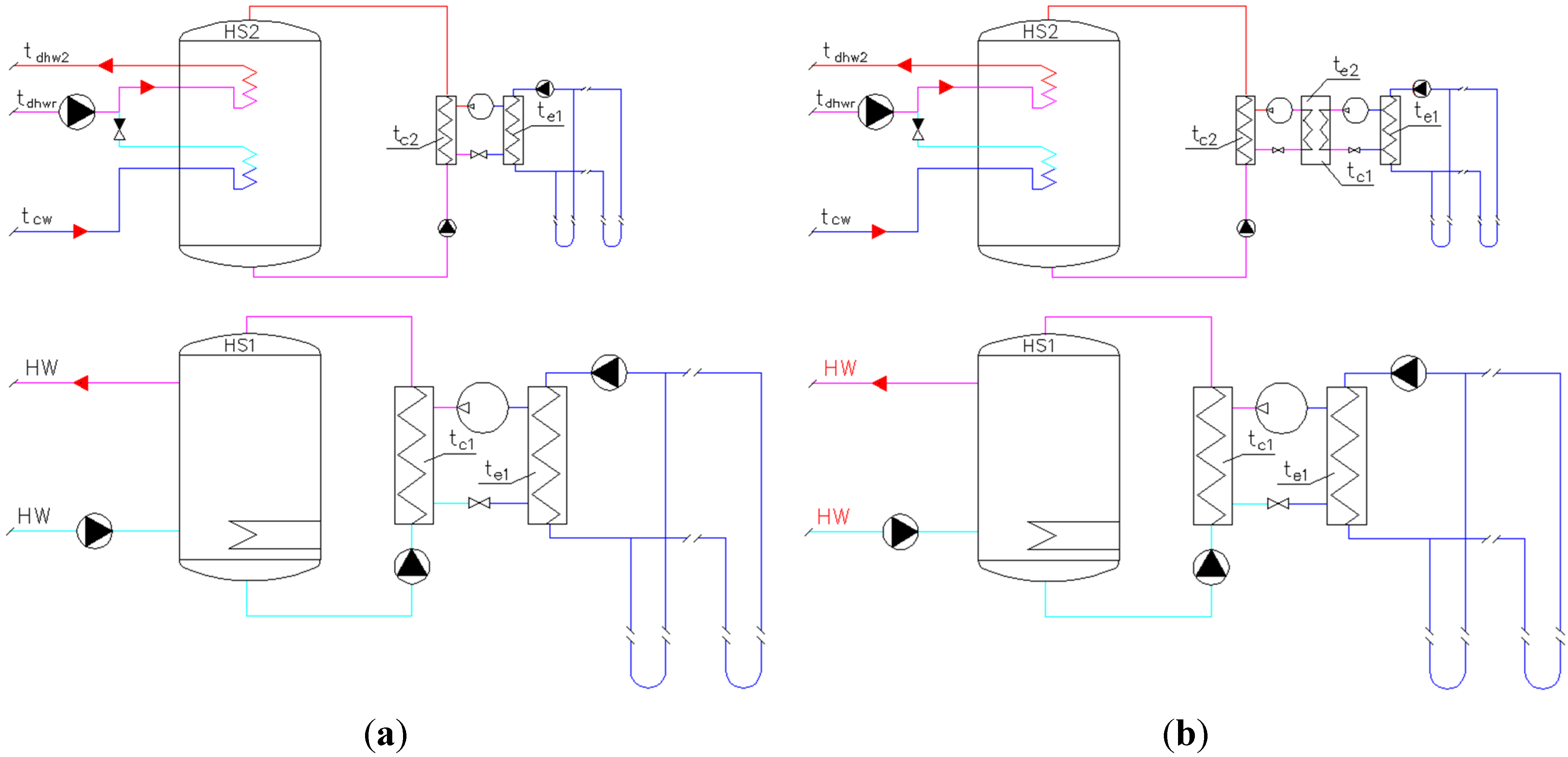
System 1: The de-superheating heat exchanger provides HT heat to heat storage 2 (HS2). The condenser provides heat to HS1, where DHW is preheated. Both storages have electric resistance heaters (
Figure 1).
System 2: The heat pump only preheats DHW in HS1, after which an electrical heater warms it up to its final temperature in HS2 (
Figure 1).
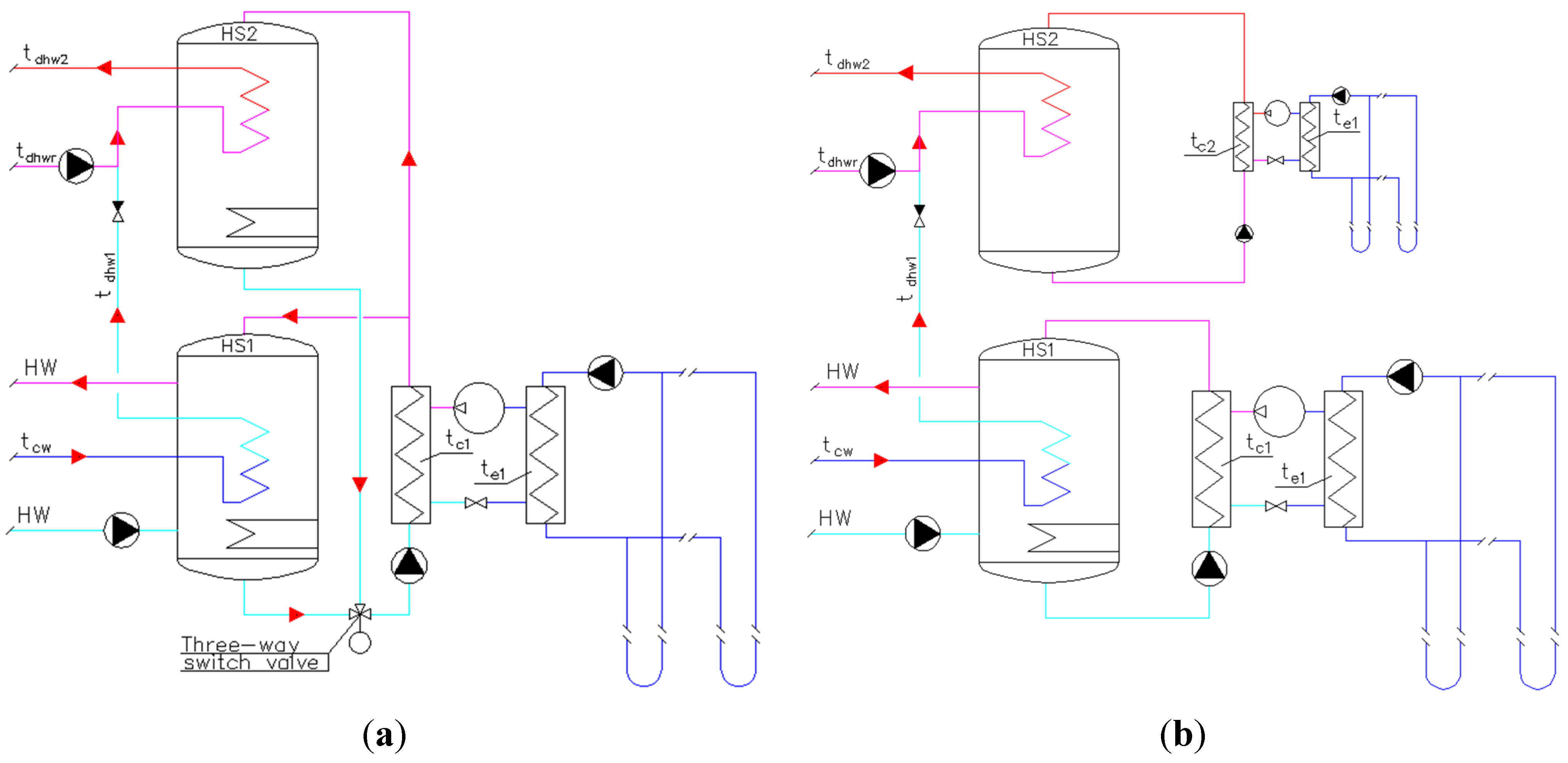
System 3: The condenser of the heat pump provides heat in turns to HS2 and HS1 by a three-way switch valve. DHW final heating in HS2 has a higher priority (
Figure 2).
Figure 1.
Domestic hot water (DHW) production: (a) System 1; and (b) System 2.
Figure 1.
Domestic hot water (DHW) production: (a) System 1; and (b) System 2.
System 4 is shown in
Figure 2, on the right. One ground-source heat pump provides heat to HS1, and the other to HS2.
Figure 2.
DHW production: (a) System 3; and (b) System 4.
Figure 2.
DHW production: (a) System 3; and (b) System 4.
In
Figure 3, two systems are shown in which all the DHW is heated in HS2. LT storage HS1 is only for the space heating system without DHW preheating. In both systems, one ground-source heat pump provides only space heating but not the DHW preheating. In System 5 the DHW heat pump is a single-stage type, and in System 6 it is the cascade type.
Figure 3.
DHW production: (a) System 5 and (b) System 6.
Figure 3.
DHW production: (a) System 5 and (b) System 6.
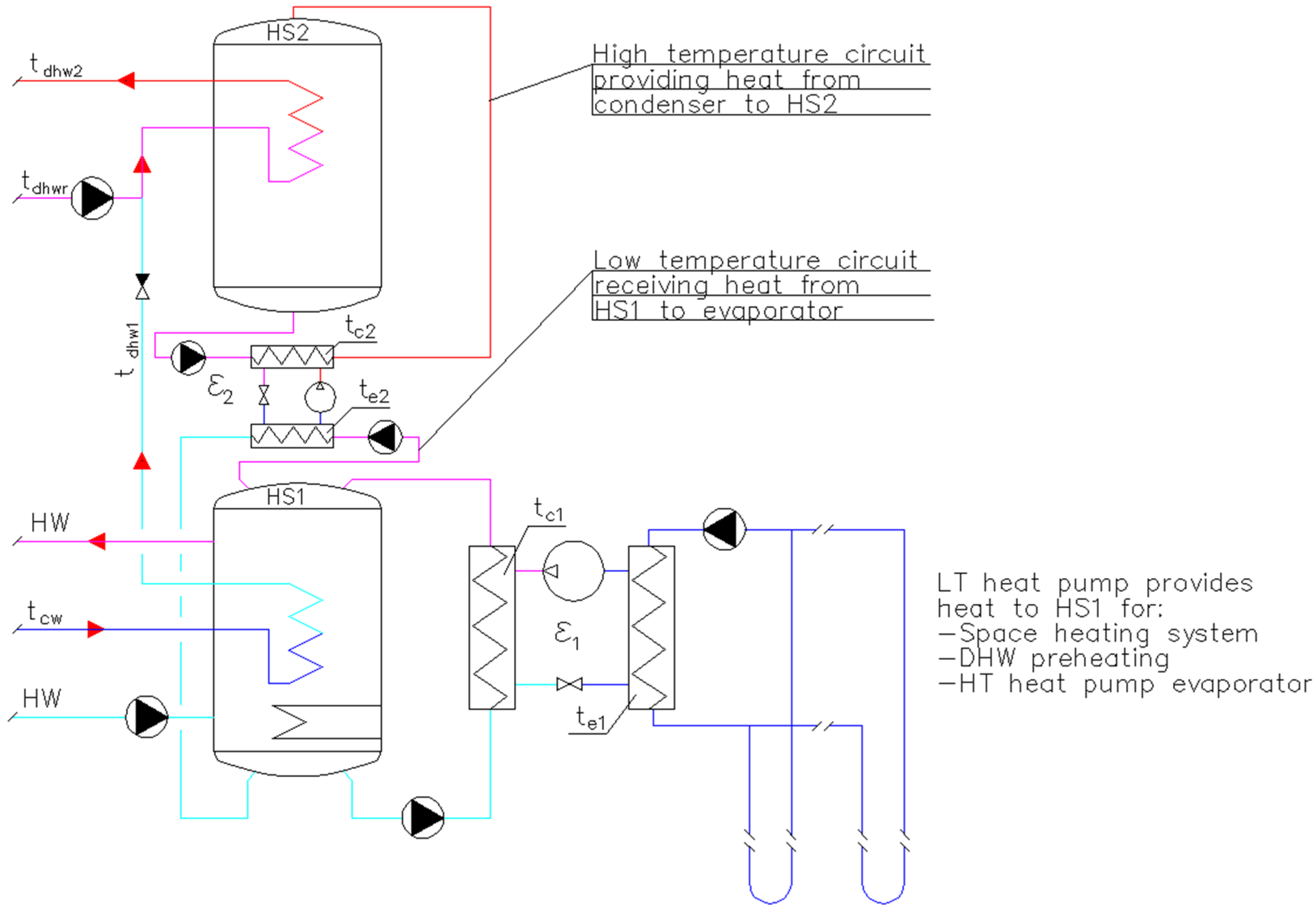
In
Figure 4, a system is suggested that combines features from Systems 4 and 6. DHW is preheated, and space heating is provided with the LT heat pump in heat storage 1. The HT heat pump provides heat for warming up the DHW to its final temperature in heat storage 2. It receives its evaporation heat from heat storage 1. Both heat pumps work with a small compression ratio, which improves the
COP of the whole system.
Figure 4.
DHW production System 7, the two-stage heat pump.
Figure 4.
DHW production System 7, the two-stage heat pump.
Bertsch and Groll [
11] have found the economizer cycle advantageous compared to intercooler and cascade cycles in the air source heat pump. However, in apartment buildings, the high loads of space heating and DHW heating are not simultaneous and the power demand of space heating and DHW preheating is higher than that of the DHW final heating. Therefore, the HT heat pump needs to run alone and it is significantly smaller in effect than the LT heat pump.
The paper proceeds as follow.
Section 2 describes the methods of choosing refrigerants and determining the performance of compressors. In addition, the calculation of the system
COP value is presented.
Section 3 presents the initial values and the results. In
Section 4, the meaning and limitations of results are discussed, and the conclusions are shown in
Section 5.
2. Analysis and Calculations
In order to avoid the freezing of groundwater in a borehole in the long term, the safe return temperature back into the ground is above −2 °C in the Finnish climate. The incoming temperature of the brine is assumed to be 3 °C. In these calculations, the evaporation temperature is kept constant at −5 °C for all the considered systems. The condensing temperature of the HT heat pump is kept constant at 65 °C.
The
COP value can be calculated with Equation (1) [
12,
13]:
where:
Qc Heat rejected by condenser (kW h)
ΣW Work done by compressor (kW h)
ηC Carnot efficiency
εC Carnot COP value
ηr Thermodynamic efficiency of refrigerant
ηis Isentropic efficiency of compressor
ηmech Mechanical efficiency of compressor
ηmotor Efficiency of electrical motor
The Carnot
COP value is calculated by using Equation (2):
where:
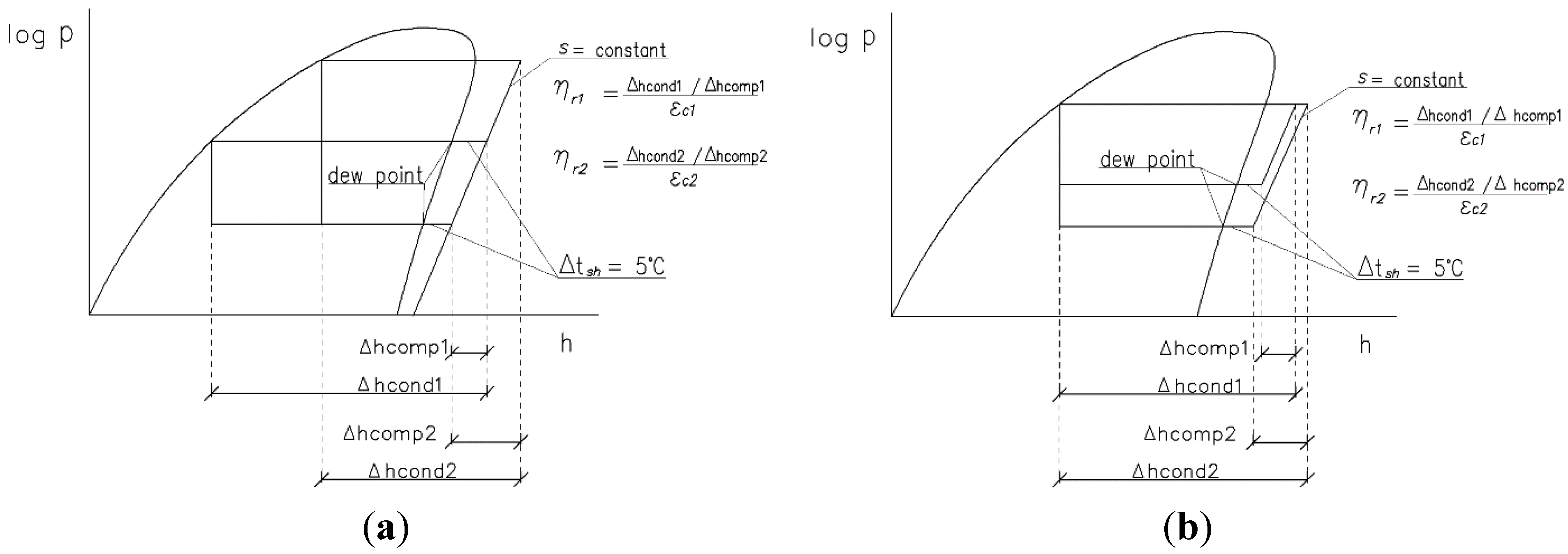
The efficiency factors in the right part of Equation (1) depend on equipment, but the thermodynamic efficiency of refrigerant η
r can be calculated with the thermal properties of the chosen refrigerant, and with the coordinates of the turning points of the cycles in the pressure-enthalpy-diagram (
Figure 5). The evaporation temperature is defined at the dew point temperature. The superheating range is kept constant at 5 °C and the sub-cooling range is 0 °C. In
Figure 5a, the evaporating temperature is constant, and in
Figure 5b, the condensing temperature is constant.
Figure 5.
Defining the thermodynamic efficiency of the refrigerant: (a) the evaporating temperature is constant; and (b) the condensing temperature is constant.
Figure 5.
Defining the thermodynamic efficiency of the refrigerant: (a) the evaporating temperature is constant; and (b) the condensing temperature is constant.
Thermodynamic efficiency ηr is used here only in order to choose the refrigerant for low- and high-stage compressors. Specific entropy s is taken as constant (ηis = 1) so that it is possible to separately define the effect of the refrigerant on the COP. This is the only efficiency factor in Equation (1) that does not depend on the compressor and its motor. The comparison of thermodynamic efficiency within the whole operating range gives information on the applicability of the refrigerant.
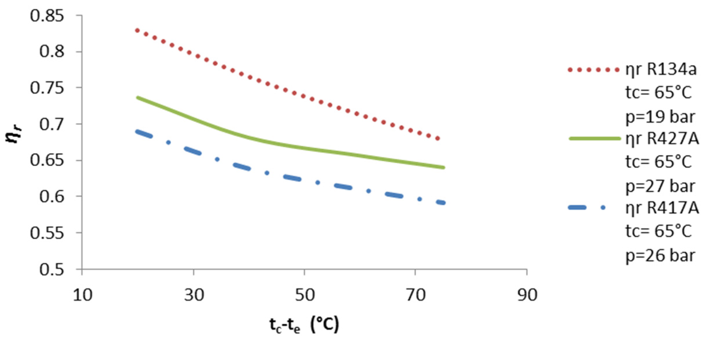
Considering the pressure, discharge temperature, solubility with lubricating oil, and the environmental aspects of the refrigerant, refrigerants R134a, R417A, and R427A are placed into the comparison of the thermodynamic efficiency with a condensing temperature of 65 °C, and R404A, R410A, and R407C with an evaporating temperature of −5 °C (
Figure 6 and
Figure 7) [
12,
13].
Figure 6.
Thermodynamic efficiency of R134a, R417A, and 427A,
tc = 65 °C [
14,
15,
16].
Figure 6.
Thermodynamic efficiency of R134a, R417A, and 427A,
tc = 65 °C [
14,
15,
16].
Figure 7.
Thermodynamic efficiency of R404A, R407C and R410A,
te = −5 °C [
16].
Figure 7.
Thermodynamic efficiency of R404A, R407C and R410A,
te = −5 °C [
16].
R134a was chosen for the HT heat pump because of its highest η
r and lowest pressure at the condensing temperature of 65 °C. R407C was chosen for the LT heat pump because of its highest η
r. Redko [
17] has suggested R407C for the cascade geothermal LT heat pump with the evaporation temperature of 20 °C and R134a for the HT heat pump with the condensing temperature of 105 °C.
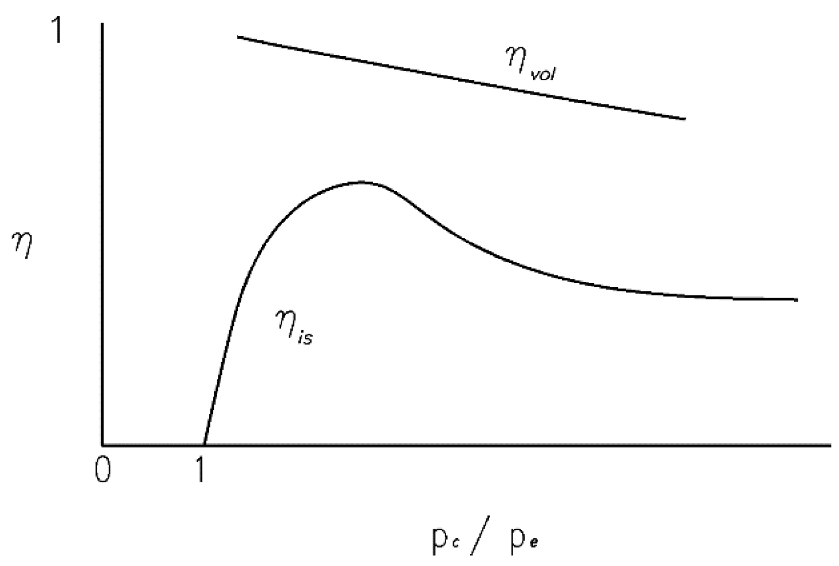
The scroll-type compressor was chosen for both the LT and the HT heat pumps because it is widely used and has good efficiency [
8]. Principle curves of isentropic and volumetric efficiencies for the scroll compressor are shown in
Figure 8. Isentropic efficiency is 0 and volumetric efficiency is 1 when the pressure ratio is 1. The isentropic efficiency increases rapidly to its maximum, and then starts to decrease slowly. However, the place and magnitude of the maximum η
is depends strongly on the selected compressor. The volumetric efficiency decreases linearly when the pressure ratio increases. Isentropic efficiency is not used in calculations but its significance is considered in
Section 2.2.
Figure 8.
The efficiency principle curves ηis and ηvol of a scroll compressor.
Figure 8.
The efficiency principle curves ηis and ηvol of a scroll compressor.
Furthermore, the mechanical efficiency of the compressor η
mech and the efficiency of the electrical motor η
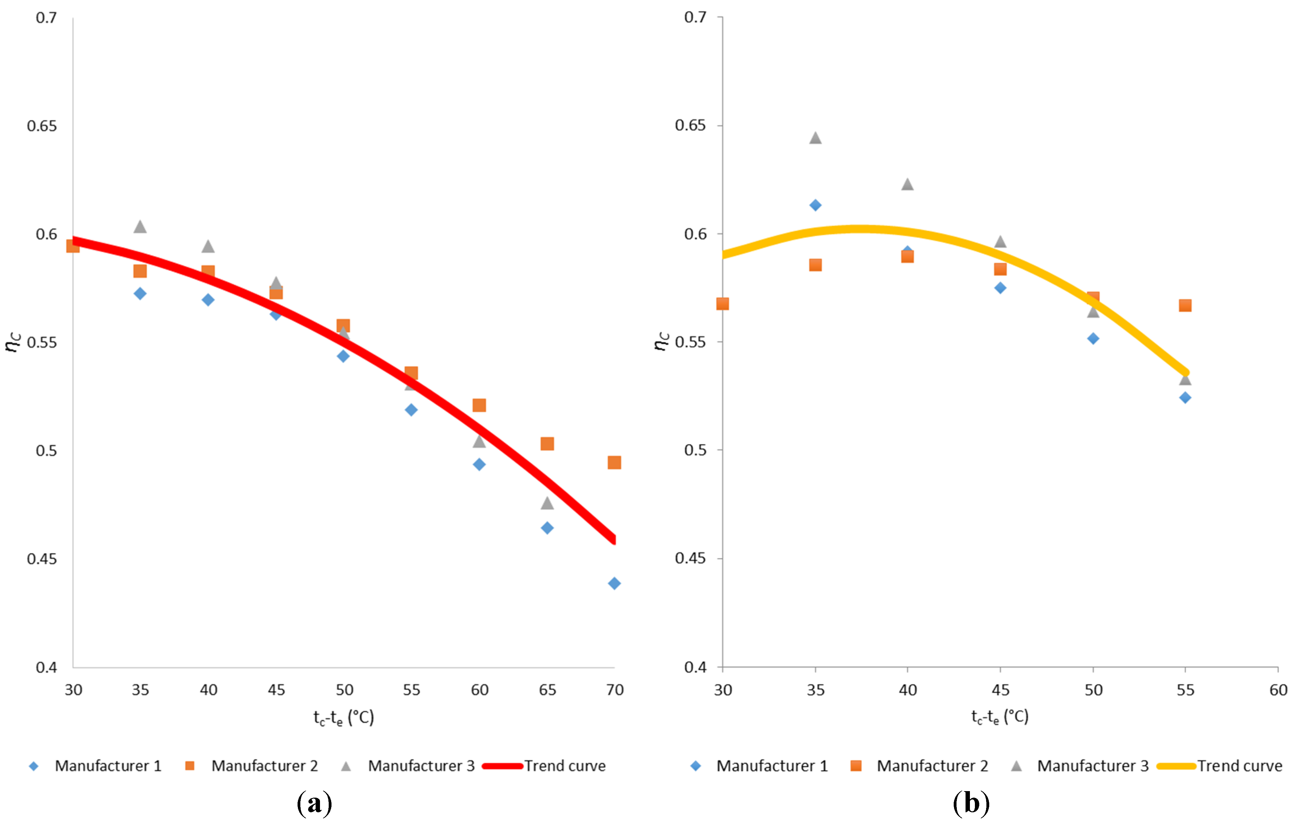
motor depend on the selected equipment. Therefore, the performance calculations are made with freely downloadable dimensioning programs from three large compressor manufacturers. The Carnot efficiencies η
C of selected scroll compressors are shown in
Figure 9. For instance, when the evaporation temperature is −5 °C and the condensing temperature is 30 °C, the highest available
COP value of compressors using R407C by Manufacturer 1 is 5.31 with Model A. The corresponding Carnot-
COP is 8.66, resulting from Equation (1) η
C = 0.61. When the condensing temperature is 50 °C, the highest available
COP is 3.08 with Model C. The corresponding Carnot-
COP is 5.88 resulting in η
C = 0.52. With the condensing temperature 35 °C, Model B has the highest performance according to the program. Thus, the dots in
Figure 9 represent a set of the highest performance compressor models from each manufacturer. The aim is to get the realistic performance values of the currently available devices for system comparisons. The regression curve is composed by spreadsheet computation. Formulas of the trend curves are given and used in the performance calculations.
Figure 9.
Carnot efficiency factor η
C for scroll compressors [
18,
19,
20]: (
a) R134a; and (
b) R407C.
Figure 9.
Carnot efficiency factor η
C for scroll compressors [
18,
19,
20]: (
a) R134a; and (
b) R407C.
2.1. System 1
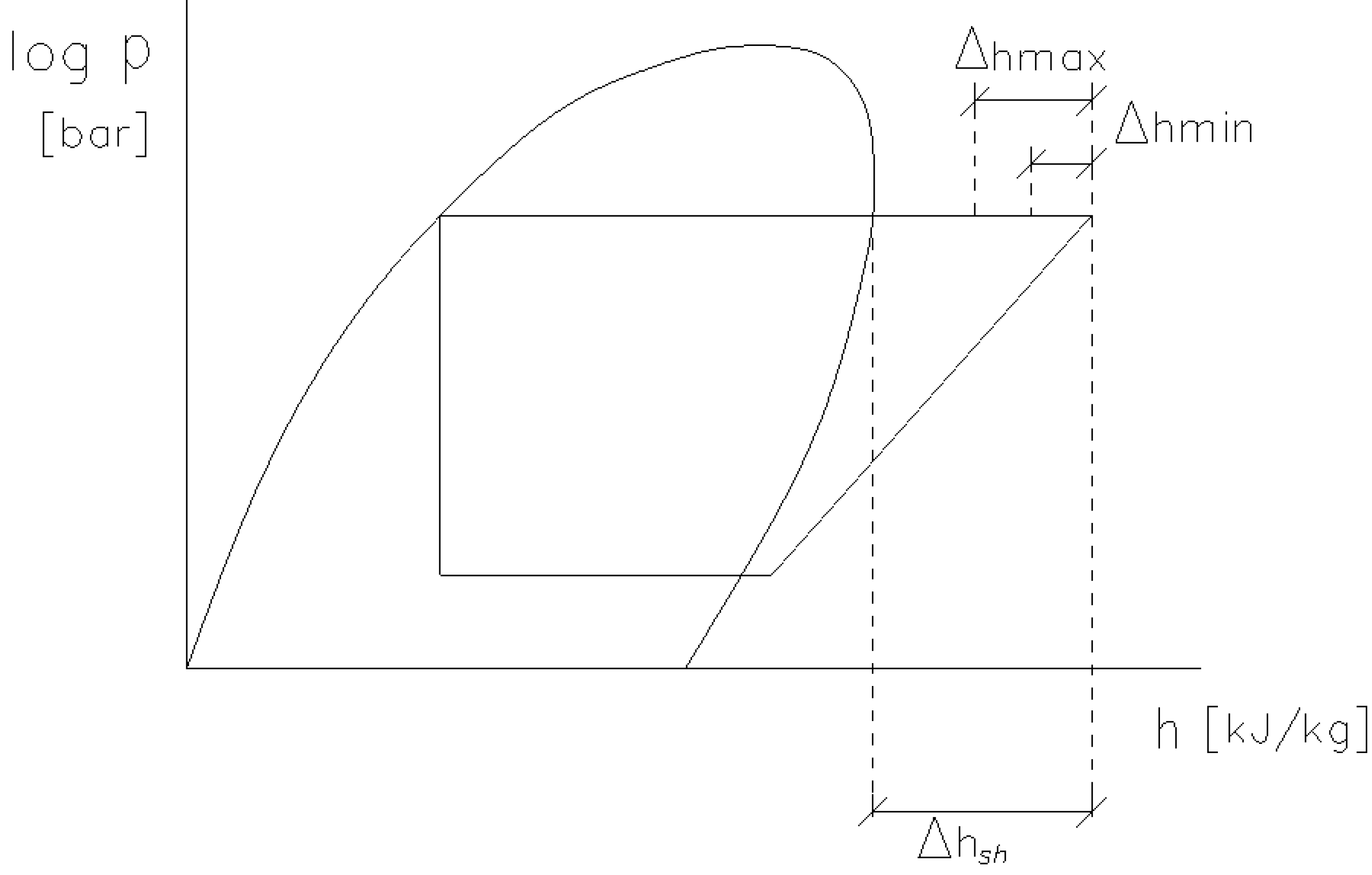
The heat output of the desuperheater is Φ
sh = qmr × Δ
h, where
qmr is the mass flow rate, and Δ
h is the enthalpy change of the refrigerant. However, the available Δ
h is smaller than Δ
hsh (
Figure 10). DHW recirculation decreases the water temperature stratification in HS1. For example, in Finland, the return temperature of recirculation water must be equal to or higher than 55 °C [
1]. Therefore, the water temperature at the bottom of HS1 may be even higher than the condensing temperature of the refrigerant. After an intensive period of DHW consumption—when the water inlet temperature into the desuperheater is the lowest—the available enthalpy change is Δ
hmax. During the night, when there is no DHW consumption, and water temperature is high and stationary, the enthalpy change is Δ
hmin and Φ
sh is equal to the sum of the heat losses of the tank and the heat demand of the recirculation water.
Figure 10.
Available enthalpy change Δhmin–Δhmax in desuperheater.
Figure 10.
Available enthalpy change Δhmin–Δhmax in desuperheater.
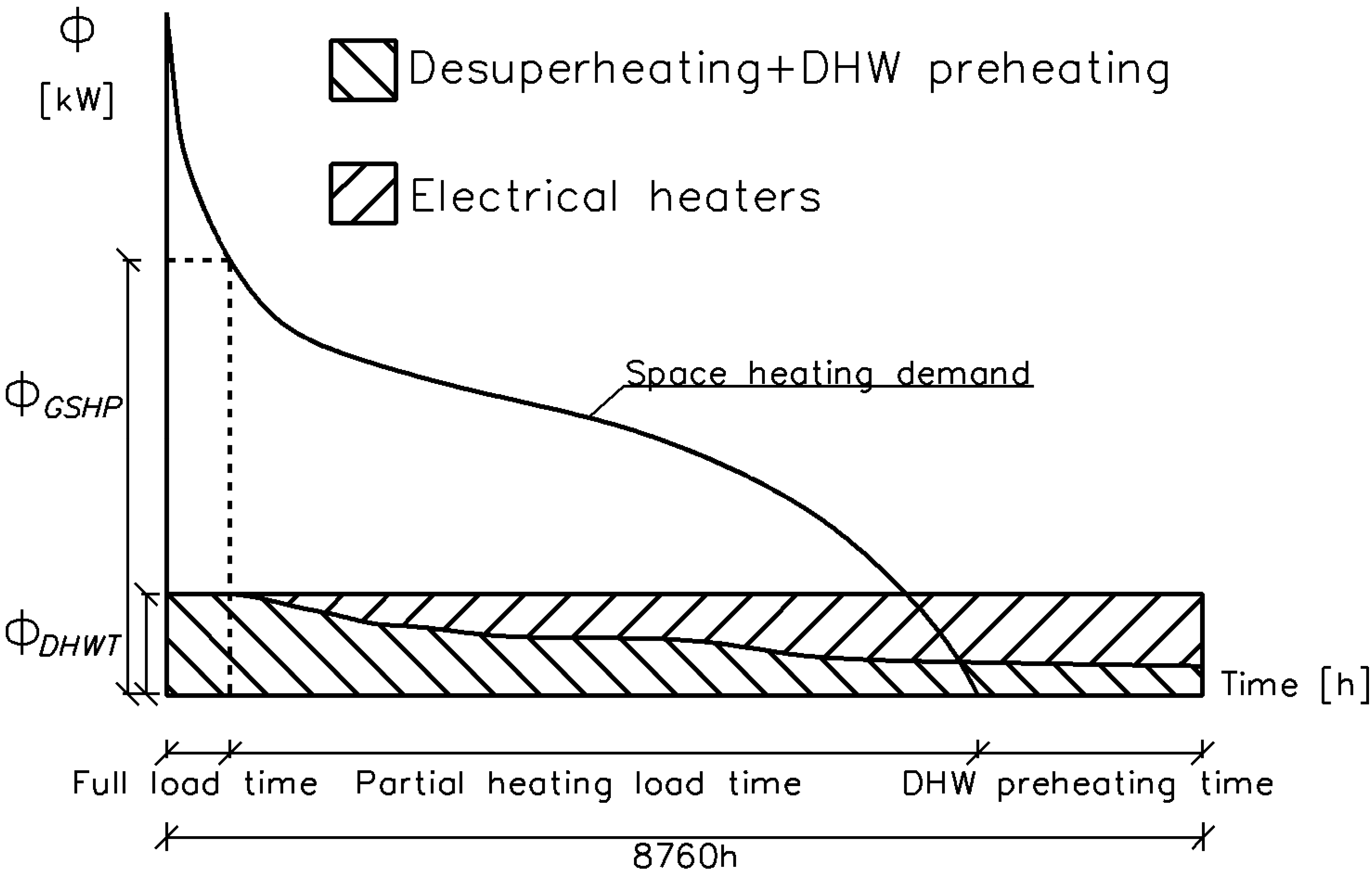
The desuperheating energy for DHW decreases when the building heat demand is low (
Figure 11). This is a significant disadvantage in System 1. In
Figure 11, the heat output of the GSHP is chosen at approximately 70% from the peak load of the building, and the full load time is the corresponding working time. It is possible to heat all the DHW during this period. The space heating duration curve shows that during the partial load time, the GSHP is working only part time (or the refrigerant mass flow rate is regulated). Therefore, it is possible to produce only a portion of the DHW heating energy by GSHP. In the summertime, condensing heat is needed only for DHW preheating, and the working periods of GSHP are very short. Paradoxically, the least amount of DHW can be heated by the desuperheater in the summertime. With System 1, electrical heating elements warm up a significant share of the DHW. This reduces the
COP value of the system. The amounts of the desuperheater and electrical heater contributions depend on the shape of the space heating power duration curve and on the power ratio of GSHP.
System 1 is not included in the COP value calculations below. The seasonal performance of System 1 depends on the factors ΦGSHP/ΦSpace Heating and ΦDHWT/ΦGSHP, which are out of the scope of this study.
Figure 11.
Exploiting possibilities of desuperheaters in DHW production.
Figure 11.
Exploiting possibilities of desuperheaters in DHW production.
2.2. Systems 2, 3, 4, and 5
The heat demand of the DHW production is calculated by using Equation (3):
Total heat demand of DHW production consists of heating demands of the used tap water and recirculation water . The former is the sum of the preheating effect and the final heating effect , which occur in storage in HS1 and HS2, respectively. The latter is the sum of heat losses in the DHW pipe network, heat storage HS2, and drying towel rails.
The
COP values for Systems 2, 3, 4, and 5 are solved by using Equation (4):
where ε
1 and ε
2 are coefficients of performance for the LT and HT stages, respectively. The share of preheating is:
where:
Heat demand of DHW preheating (kW)
Heat demand of DHW recirculation (kW)
ĊDHW Heat capacity flow rate of DHW (kW/K)
tDHW1 Preheated DHW temperature (°C)
tCW Domestic cold water temperature (°C)
tDHW2 Final temperature of DHW (°C)
ĊDHWR Heat capacity flow rate of DHW recirculation (kW/K)
tDHWR DHW return temperature (°C)
Examples of COP value calculations are shown below.
2.2.1. System 2
The DHW is heated to the final temperature by an electrical heater, and thus ε
2 = 1. The condensing and evaporation temperatures are
tc1 = 35 °C and
te1 = −5 °C, which gives ε
C1 = 7.70 with Equation (2) and η
C1 = 0.60 from
Figure 9. Their product is ε
1 = ε
C1η
C1 = 4.63. The DHW temperatures are
tDHW1 = 33 °C and
tDHW2 = 60 °C. Heat capacity flow
ĊDHW = 13,304 W/(60 − 5) °C = 242 W/°C. Then factor
a and the
COP value can be calculated with Equations (4) and (5):
2.2.2. System 3
There are three different operation strategies of System 3:
(1) There is no preheating coil and the heat pump operates producing warm water at the same temperature either for the space heating system or for the DHW system. Final heating is carried out by electrical heater. With this strategy, the performance is equal to System 2.
(2) The condensing temperature is chosen to be high enough for DHW purposes and it remains constant. With this strategy, the performance for the part of DHW production is equal to System 5. However, as for space heating, the condensing temperature is unnecessarily high. Therefore, this strategy is not reasonable if both spaces are heated and DHW is produced with a GSHP.
(3) The condensing temperature changes. When the three-way valve regulates flow into HS2, the condensing temperature is controlled to be 65 °C, and when it regulates flow into HS1, the condensing temperature is controlled by the need of the space heating system. Both η
r and η
is are changing, respectively. If the compressor model is chosen to operate at highest η
is with the high condensing temperature (high value of
pc/
pe), the isentropic efficiency may decrease crucially with the low condensing temperature (
Figure 8), and
vice versa, if the compressor model is chosen to give its highest η
is at a low condensing temperature, the isentropic efficiency may decrease with the high condensing temperature. The performance of the systems is calculated with the regression curves of the Carnot efficiency value in
Figure 9, where the optimal compressor model is chosen for every operating temperature. However, with this approach, it is not known how one compressor model performs when operating outside of its optimal conditions and how the condensing temperature changes during the operating period. Therefore, System 3 is not included in the performance calculations. However, it can be concluded that the performance of this running strategy is lower than that of System 4 but higher than that of System 5.
2.2.3. System 4
All the other values are equal with System 2, but the ε2 value is higher because heat is delivered into HS2 by the HT heat pump. Here, tc2 = 65 °C and te2 = −5 °C, resulting in εC2 = 4.83, ηC2 = 0.46, ε2 = 2.22, and COPS4 = 2.83, respectively.
2.2.4. System 5
Here a = 0 because all heating of DHW and DHWR is carried out by the HT heat pump, which has the same operating conditions as System 4. Thus, ε2 = 2.22 and it equals the COP value of the system, resulting in COPS5 = 2.22.
2.3. Systems 6 and 7
COP values for Systems 6 and 7 are solved with Equation (6):
where:
QDHW Energy demand of DHW (kW h)
QDHWR Energy demand of DHW recirculation (kW h)
WLT Work by LT stage (kW h)
WHT Work by HT stage (kW h)
ε1 COP for LT stage
ε2 COP for HT stage
a The share of preheating
2.3.1. System 6
In cascade System 6, the low-stage operating temperatures are equal with Systems 2 and 4, following the same performance with ε
1 = 4.63. Here, heat transfers from R407C directly to R134a and thus
te2 = 30 °C following η
C2 = 0.59, ε
C2 = 9.7, and ε
2 = 5.70, respectively. In cascade System 6, factor
a = 0 and the
COP value is:
2.3.2. System 7
In the System 7, the low-stage operating temperatures are also equal with Systems 2 and 4, following the same performance with ε
1 = 4.63. However, here heat transfers from R407C to the water in HS1 and from the water to R134a and thus
te2 = 25 °C, following η
C2 = 0.58, ε
C2 = 8.45, and ε
2 = 4.90, respectively. In System 7,
a = 0.407 and the
COP value is:
Even if the cascade system gets benefits by avoiding one temperature step, the overall performance is better in System 7. This is due to preheating the DHW with the LT heat pump with a low pressure ratio and good efficiency.
The heat loss of HS2 is included in the heat losses of the recirculation pipe network. The energy consumption of the circulation pumps is not included.
3. Results
The performances of the systems are compared by changing factor
b = Φ
DHWR/Φ
DHWT and temperature
tc1. The temperatures used in the comparison calculations are shown in
Table 1. The temperature difference between the condensing refrigerant and the leaving water is chosen as 2 °C, but between the incoming brine or water and the evaporating refrigerant it is chosen as 8 °C. Without sub-cooling, the former does not increase the conductance demand of the condenser to excess and the latter ensures sufficient superheating of the suction gas. Instead, in the cascade system, the temperature difference between condensing R407C and evaporating R134a is chosen to be 5 °C. This is assumed to ensure sufficient superheating of R134a suction gas due to the higher temperature of incoming superheated R407C.
Table 1.
System descriptions and temperatures. LT: low temperature; and HT: high temperature.
Table 1.
System descriptions and temperatures. LT: low temperature; and HT: high temperature.
| System | DHW preheating | DHW final heating and heating of recirculating DHW | tc2 (°C) | tdhw2 (°C) | tdhwr (°C) | tc1 (°C) | te2 (°C) | tdhw1 (°C) | tcw (°C) | te1 (°C) |
|---|
| 2 | Heat pump 1 LT | Electrical heater | - | 60 | 55 | 25–50 | - | 23–48 | 5 | −5 |
| 3 | Heat pump 1 HT | Heat pump 1 HT | - | 60 | 55 | 65 | - | - | 5 | −5 |
| 4 | Heat pump 1 LT | Heat pump 2 HT | 65 | 60 | 55 | 25–50 | −5 | 23–48 | 5 | −5 |
| 5 | * | Heat pump 2 HT | - | 60 | 55 | 65 | −5 | - | 5 | - |
| 6 | * | Cascade heat pump 2 HT | 65 | 60 | 55 | 25–50 | 20–45 | - | 5 | −5 |
| 7 | Heat pump 1 LT | Heat pump 2 HT | 65 | 60 | 55 | 25–50 | 15–40 | 23–48 | 5 | −5 |
Factor
b—the share of recirculating DHW heating power from the total DHW heating power demand—depends on the length and insulation of the pipe network, the amount of drying towel rails or other heating coils, and the insulation of HS2. With short and well-insulated pipelines, and without towel rails, it is possible to achieve a low value for factor
b, e.g.,
b = 0.1. If there is a towel rail in every apartment and pipelines are long and poorly insulated, factor b is high, e.g.,
b = 0.6.
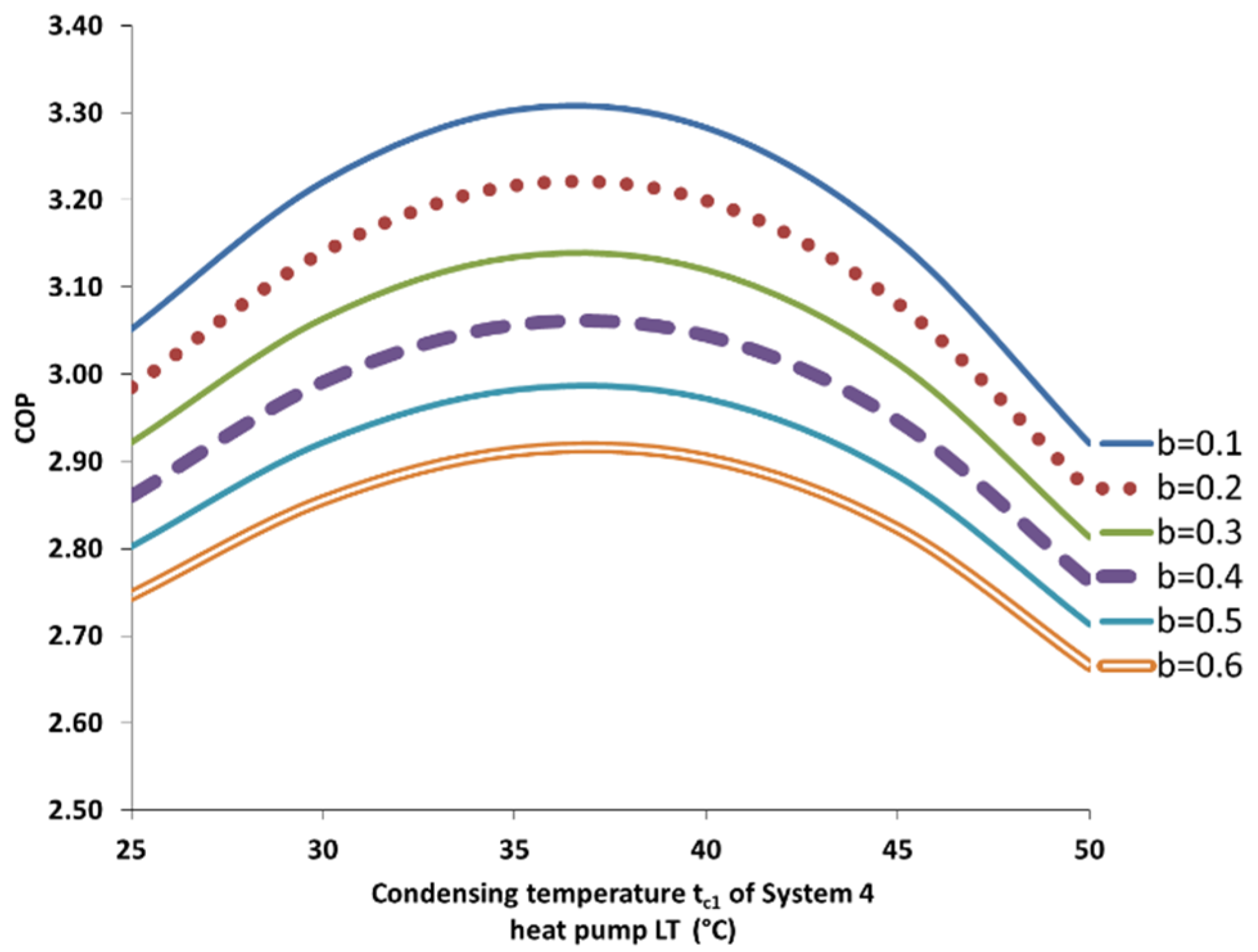
COP values of System 7 are shown in
Figure 12 with different condensing temperatures and factor
b as a parameter.
Figure 12.
Coefficient of performance (COP) values of System 7.
Figure 12.
Coefficient of performance (COP) values of System 7.
The optimal condensing temperature proved to be 35–37 °C. This result is in reasonable accordance with the experimental study concerning the optimum intermediate temperature of R410A (LT)/R134a (HT) air to the water cascade heat pump [
21]. The
COP value decreases by approximately 5% if
tc1 is either increasing or decreasing by 10 °C from the optimum. The
COP value increases by approximately 12% if factor b decreases from 0.6 to 0.1, and
tc1 is within the optimal range. This change is smaller with lower or higher temperatures.
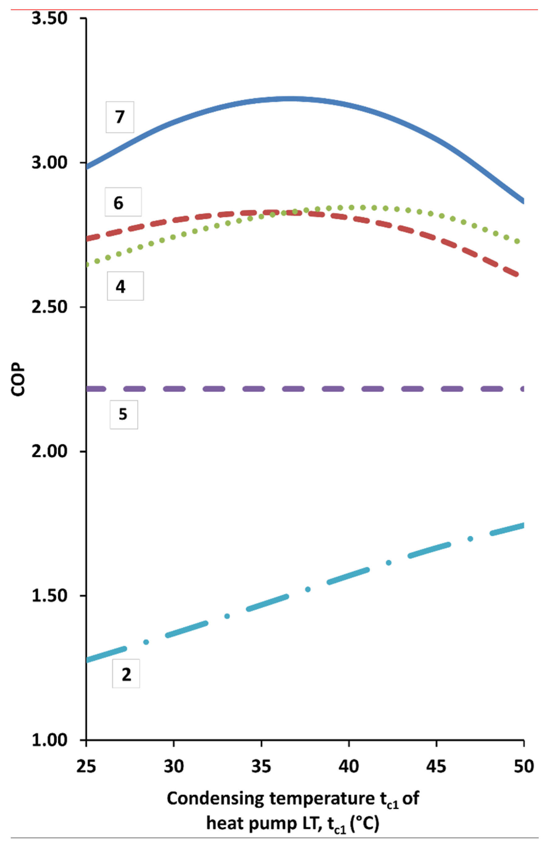
Factor
b = 0.2 is chosen for the system performance comparison calculations because it is possible to achieve that with reasonable insulation thickness (
Figure 13).
Figure 13.
Comparison of COP values.
Figure 13.
Comparison of COP values.
The COP value for System 2 is the poorest due to the electrical heater, but it improves from 1.28 to 1.74 when tc1 increases from 25 °C to 55 °C, i.e., the share of preheating a by the heat pump increases from 0.26 to 0.63.
With System 5, the total heat demand of DHW ΦDHWT is supplied by HT heat pump 2 when LT heat pump 1 operates only for space heating. This results in a COP value of 2.22, and factor b has no effect on the result.
The performance curve of System 4 is rising because the performance of LT heat pump 1 is higher than that of HT heat pump 2. The curve reaches its maximum
COP value of 2.84 when
tc1 is 40 °C,
i.e.,
a = 0.48. Then it starts to decrease because in addition to ε
C1 decreasing, η
C1 also begins to decrease (
Figure 9). However, the
COP value is then higher than that of System 6. The reason for this is that the cascade heat pump transfers all the energy at a HT (
a = 0) when LT heat pump 1 in System 4 transfers a significant share at a lower temperature. This effect is smaller when
tc1 = 25–35 °C, and the
COP value of the cascade heat pump is higher. At
tc1 = 35 °C, the systems are equal.
System 7 combines the advantages of cascade Systems 4 and 6. First, heat pumps 1 and 2 work in a series connection. Although 5 °C are lost due to heat transfer in the additional heat exchanger, εC and ηC of both heat pumps remain at a high level. The operating temperatures of the LT stage, and thus also εC and ηC, are equal in Systems 6 and 7. Secondly, the DHW is heated in two stages. Accordingly, System 7 yields the highest COP value at all considered temperatures tc1. At the optimum temperature, the electrical power savings are 12% compared with Systems 4 and 6, 31% compared with System 5, and 54% compared with System 2.
4. Discussion
This system approach study concerns various arrangements of GSHPs as part of the heating system in an apartment building. The internal improvement methods of the cycle, e.g., sub-cooling or internal heat exchanger, are not considered. These methods are available for all the considered systems, so they are not assumed to change the ranking of the systems. On the other hand, the energy use of the pumps is excluded, which decreases the
COP values shown in
Figure 13. The brine pump is the most powerful and its volume flow rate increases if the
COP value improves. Other pumps are relatively small in effect.
The investment costs are excluded from this study, but there are some beneficial features concerning the price of System 7. The size of heat pump 1 (LT) is determined mainly by the heat demand of space heating, so the price differences between these compressors are marginal costs. However, the volume flow rate of heat pump 2 (HT) is higher in Systems 4 and 5 than in System 7 because the specific volume of R134a suction gas is approximately 2.5-fold larger at the pressure of evaporation temperature
te = −5 °C than that of
te = 25 °C. Further, the ε
2 of heat pump 2 (HT) is more than double in System 7 than in Systems 4 and 5. Therefore, the size of the compressor is significantly smaller in System 7 than that in Systems 4 and 5. Regarding Systems 6 and 7, cascade heat pump 2 (HT) includes two compressors and other additional devices, and thus System 6 is more expensive. Instead, life cycle cost calculations are needed to clarify the profitability order between Systems 1, 2, 3, and 7. A rough evaluation in a medium-size apartment building is shown in
Table 2 to exemplify the magnitude of the DHW production energy costs. The energy costs of System 1 lie between Systems 2 and 5. The energy costs of System 3 lie between Systems 4 and 5.
Table 2.
The DHW production energy costs with different heat pump systems.
Table 2.
The DHW production energy costs with different heat pump systems.
| Building volume | 10,000 | m3 | Average ΦDHW | 13,304 | W |
| Number of apartments | 50 | - | ΦDHWR | 3350 | W |
| Number of inhabitants | 100 | - | QDHWT | 146 | MW h/a |
| DHW consumption | 5000 | dm3/d | Annual energy costs | - | - |
| Heat loss of HS2 | 500 | W | Electrical heater (COP = 1) | 16,048 | €/a |
| Length of DHW circulation pipeline | 375 | m | System 2 (COP = 1.47) | 10,917 | €/a |
| Average heat loss of circulation pipeline | 6 | W/m | System 5 (COP = 2.22) | 7229 | €/a |
| Number of drying towel rails | 3 | | System 4 (COP = 2.81) | 5711 | €/a |
| Heat loss of one drying towel rail | 200 | W | System 6 (COP = 2.83) | 5671 | €/a |
| Electrical energy price | 110 | €/MW h | System 7 (COP = 3.14) | 5111 | €/a |
Development work is needed in System 7 because of the high evaporation temperature
te2. Most of the scroll compressors are designed for evaporation temperatures below 20 °C. Exceeding this leads to motor overload. However, there are cascade heat pumps available, where the HT stage works with R134a to produce a hot water at temperature of 60 °C or higher [
22]. Goričanec
et al. [
23] has proposed a cascade heat pump where the refrigerant of the HT heat pump is R600a with the evaporating temperature at approximately 32 °C.
System 7 provides the possibility of producing the whole DHW amount with a high
COP value. The LT or HT compressor can run alone, which is not possible in most cascade or other two-stage heat pumps. This independent running feature also simplifies the controlling of the system. Utilizing water tanks lengthens the running periods of compressors, which is beneficial if on/off cycling is in use [
24]. To maximize the performance of System 7, it is essential first to avoid drying towel rails and other heating coils in the recirculation network, and secondly, to insulate the DHW and recirculation pipelines well. Finally, it is advantageous to design the space heating system for a low supply water temperature. The optimum condensing temperature for heat pump 1 (LT) is high enough for floor heating, for LT radiator heating, and for heat exchangers of supply air in nearly zero-energy buildings and low-energy buildings. On the other hand, it is also possible to use HS2 for heating the supply water of the space heating system to a higher temperature, but this is not considered here.
5. Conclusions
The share of the DHW production in the total heat consumption of the building has increased in new low-energy apartment buildings, and the temperature of the DHW is higher than that of the space-heating supply water. Therefore, DHW production has become more important in heating system design. Alternative GSHP arrangements for DHW production are described and analyzed in this study.
A two-stage heat pump system is introduced with which DHW can be produced with approximately 31% less electricity consumption than with the single-stage heat pump. Typically, there are two water tanks in the GSHP heating system: one acting as heat storage for the space heating system, and the other for the DHW system. In this system, two single-stage heat pumps are connected in a series, utilizing these water tanks. The LT heat pump, with refrigerant R407C, operates between the ground source and LT tank HS1, and the HT heat pump with R134a operates between the tanks HS1 and HS2. The DHW is preheated in the LT tank HS1, and finally heated again in the HT tank HS2, where the recirculating DHW is also heated. Both heat pumps can run alone.
In addition, the electricity consumption is 12% less than with the cascade heat pump system, even if one temperature step is lost due to transferring heat from the condenser to the water and only then to the refrigerant in the evaporator of the HT heat pump. Preheating DHW with the LT heat pump with a low pressure ratio and high COP value compensates this loss. When the evaporating temperature of the LT heat pump is a constant −5 °C, and the condensing temperature of the HT heat pump is a constant 65 °C, the system performance depends on the intermediate condensing/evaporating temperature between the stages. The optimum condensing temperature of the LT heat pump proved to be 35–37 °C, which is high enough for a LT heat distribution network in nearly zero-energy buildings or low-energy buildings. System 7 provides a possibility to produce the whole amount of DHW with a high COP value. To maximize the performance of System 7, it is essential to avoid drying towel rails and other heating coils in the recirculation network, and to insulate the DHW and recirculation pipelines properly. Investment costs are not included in calculations.


