In this section, firstly six commonly used benchmark functions are used to test the performance of the proposed improved ABC algorithm. Then, the I-V characteristic of a diameter commercial silicon solar cell is used to evaluate the efficiency of the proposed parameter identification method. All the experiments in this paper were run on the same hardware (Intel Core i3-2310 Quad with 2.1 GHz CPU and 2 GB memory).
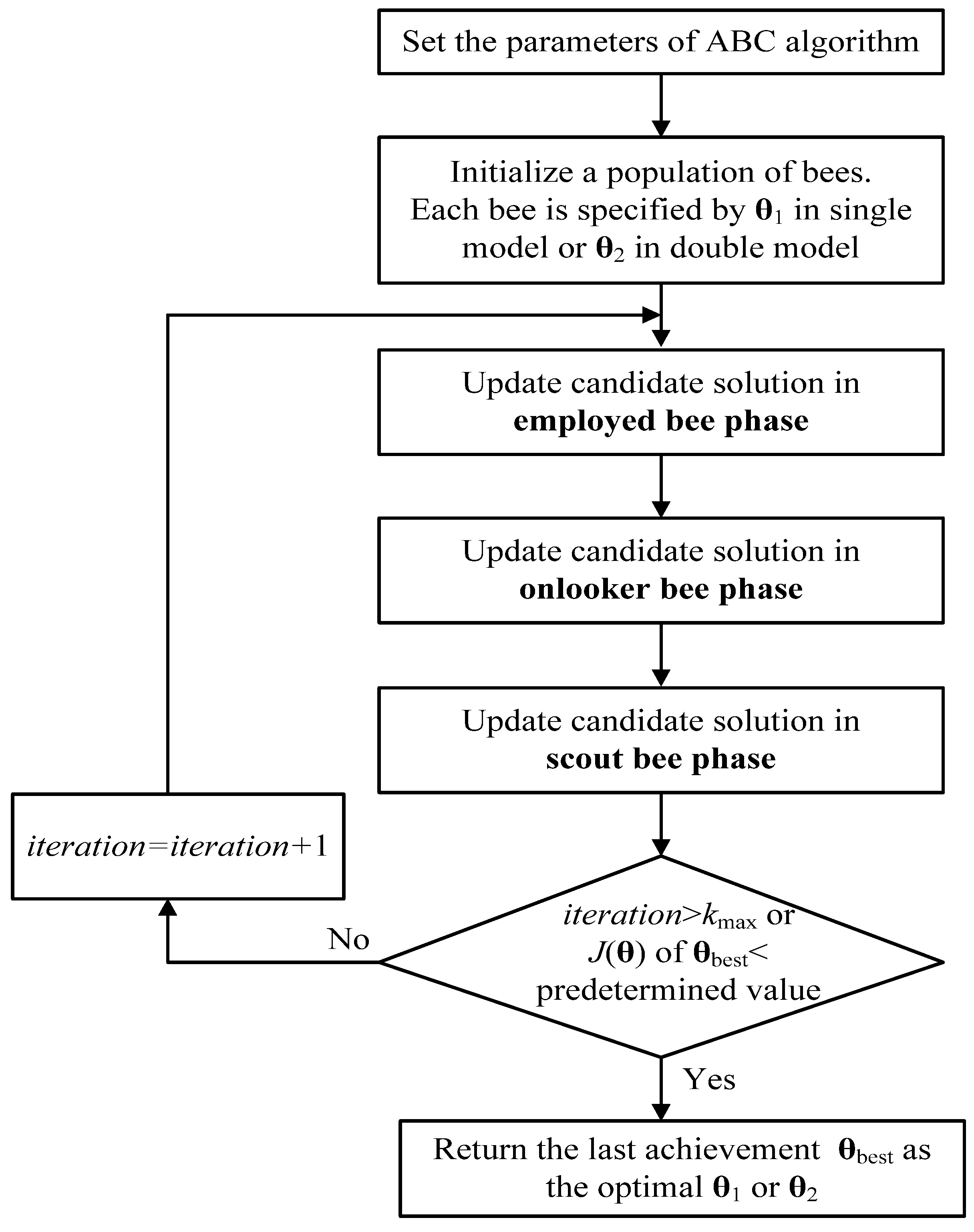
4.1. Numerical Experiments and Results
Unimodal and multimodal benchmark functions as shown in Equations (11)–(16) were used in this experiment. The aim is to minimize
fi(
β),
I = 1, 2, …, 6. We validate the performance of improved ABC algorithm (IABC) by comparing it with the origin ABC algorithm in [
14], DE in [
12], and PSO in [
16]. The control parameters in these algorithms are given in
Table 2.
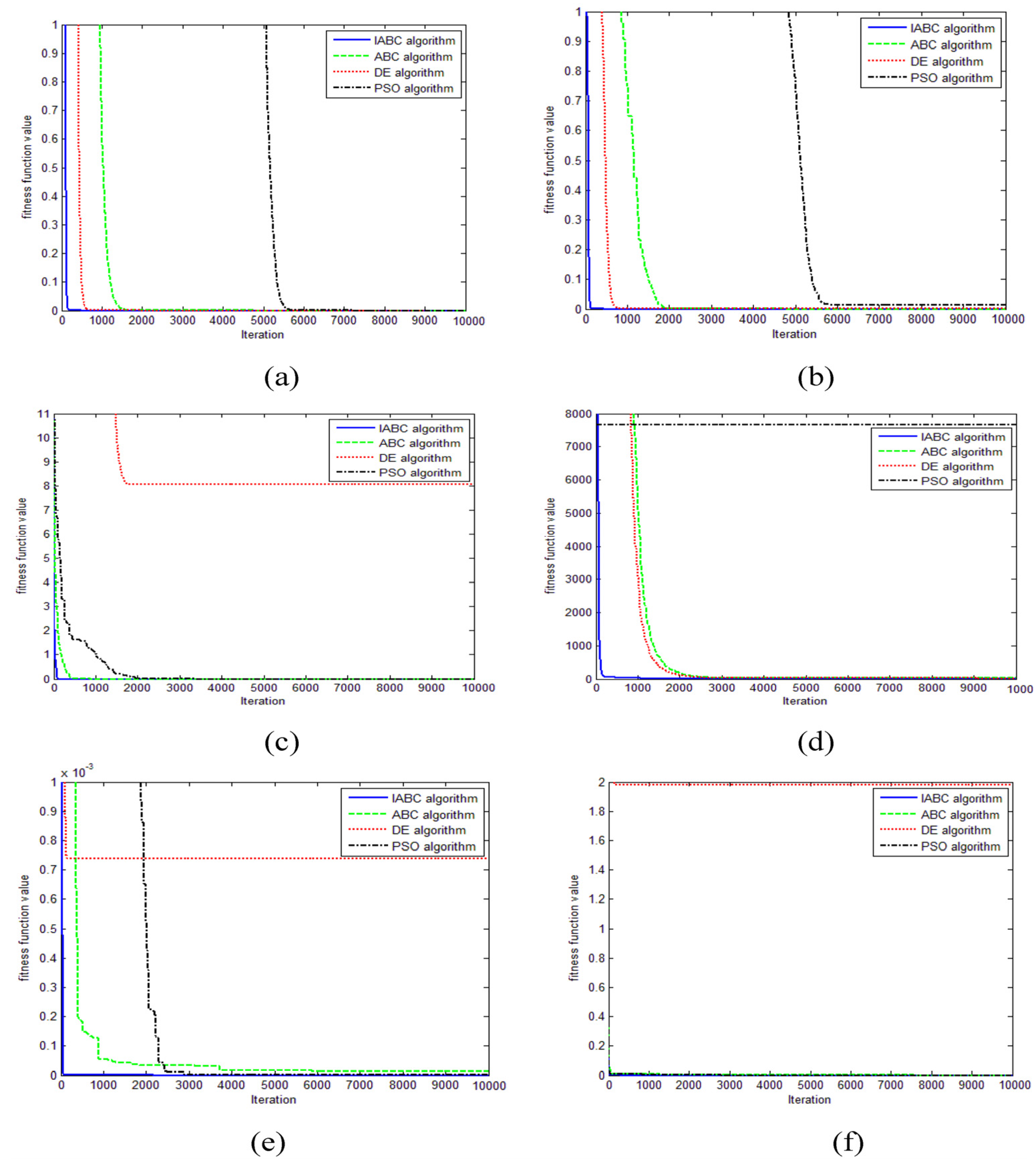
Figure 5 shows the comparison of the convergence speed of four different optimization algorithms.
Table 3 presents the mean and standard deviation of the 20 runs of the four optimization algorithms on the six functions. The “Mean” column is the average output values of benchmark functions. The “Std” column shows the standard deviation of the results. Moreover, “Best”, “Median” and “Worst” of solutions obtained in the 20 runs by each algorithm.
Sphere function:
where the range of
β is [−100 100]
D,
D = 30. The global minimum of the Sphere function is 0, and its characteristic is unimodal and separable.
Griewank function:
where the range of
β is [−600 600]
D,
D = 30. The global minimum of the Griewank function is 0, and its characteristic is multimodal and non-separable.
Ragstrigin function:
where the range of
β is [−5.12 5.12]
D,
D = 4. The global minimum of the Ragstrigin function is 0, and its characteristic is multimodal and separable.
Figure 5.
Convergence curve of difference optimization algorithms: (a) Sphere function; (b) Griewank function; (c) Ragstrigin function; (d) Rosenbrock function; (e) Ackley function; (f) Schaffer function.
Figure 5.
Convergence curve of difference optimization algorithms: (a) Sphere function; (b) Griewank function; (c) Ragstrigin function; (d) Rosenbrock function; (e) Ackley function; (f) Schaffer function.
Table 2.
Control parameters of optimization algorithm.
Table 2.
Control parameters of optimization algorithm.
| Algorithm | Parameters |
|---|
IABC
ABC | Population size = 30
klimit = 5 |
| DE | Population size = 30
Mutation factor = 2
Crossover constant = 0.5 |
| PSO | Population size = 30
Learning factors c1 = c2 = 2
Inertia weight taken from 0.9 to 0.4 |
Table 3.
Comparison of testing result of different optimization algorithms.
Table 3.
Comparison of testing result of different optimization algorithms.
| Benchmark Function | IABC Algorithm | ABC Algorithm | DE Algorithm | PSO Algorithm |
|---|
| Sphere function | Best | 0 | 5.8688 × 10−40 | 0 | 2.3404 × 10−63 |
| Median | 0 | 2.5194 × 10−39 | 4.7858 × 10−103 | 3.4396 × 10−60 |
| Worst | 0 | 1.9346 × 10−38 | 9.8389 × 10−102 | 5.0652 × 10−58 |
| Mean | 0 | 4.8372 × 10−39 | 1.6817 × 10−102 | 5.4403 × 10−59 |
| Std | 0 | 5.8316 × 10−39 | 3.0304 × 10−102 | 1.5894 × 10−58 |
| Griewank function | Best | 0 | 0 | 0 | 0 |
| Median | 0 | 0 | 0 | 0.0148 |
| Worst | 0 | 0 | 0.0123 | 0.0319 |
| Mean | 0 | 0 | 0.0020 | 0.0130 |
| Std | 0 | 0 | 0.0043 | 0.0123 |
| Ragstrigin function | Best | 0 | 0 | 4.9748 | 0 |
| Median | 0 | 0 | 8.4572 | 0 |
| Worst | 0 | 0 | 9.9496 | 0 |
| Mean | 0 | 0 | 8.0592 | 0 |
| Std | 0 | 0 | 1.7829 | 0 |
| Rosenbrock function | Best | 3.0402 | 21.4035 | 5.0174 × 10³ | 5.2015 × 10³ |
| Median | 3.0402 | 23.0599 | 6.0455 × 10³ | 7.7961 × 10³ |
| Worst | 3.0402 | 23.9106 | 7.0165 × 10³ | 9.0812 × 10³ |
| Best | 3.0402 | 22.9217 | 6.0143 × 10³ | 7.6646 × 10³ |
| Median | 1.5736 × 10⁻¹⁵ | 0.6897 | 738.2365 | 1.0434 × 10³ |
| Ackley function | Best | 0 | 0 | 0 | 0 |
| Median | 0 | 2.8194 × 10⁻⁹ | 0 | 2.2204 × 10⁻¹⁶ |
| Worst | 0 | 1.3155 × 10⁻⁴ | 0.0074 | 1.7764 × 10⁻¹⁵ |
| Best | 0 | 1.3264 × 10⁻⁵ | 7.3960 × 10⁻⁴ | 6.6613 × 10⁻¹⁶ |
| Median | 0 | 4.1560 × 10⁻⁵ | 0.0023 | 8.1752 × 10⁻¹⁶ |
| Schaffer function | Best | 0 | 0 | 1.9800 | 0 |
| Median | 0 | 0 | 1.9800 | 0 |
| Worst | 0 | 0 | 1.9800 | 0 |
| Mean | 0 | 0 | 1.9800 | 0 |
| Std | 0 | 0 | 1.4803 × 10⁻¹⁶ | 0 |
Rosenbrock function:
where the range of
β is [−30 30]
D,
D = 30. The global minimum of the Rosenbrock function is 0, and its characteristic is unimodal and non-separable.
Ackley function:
where the range of
β is [−32 32]
D,
D = 2. The global minimum of the Ackley function is 0, and its characteristic is multimodal and non-separable.
Schaffer function:
where the range of
β is [−100 100]
D,
D = 2. The global minimum of the Schaffer function is 0, and its characteristic is multimodal and non-separable.
In
Table 3, we compare the results using the same number of iterations. The Mean is relatively low, which implies faster convergence speed among experimental runs. The Std is relatively low, which implies higher consistency among experimental runs. The Best, Median and Worst are relatively low, which implies a better quality solution than other algorithms among experimental runs. The results in
Figure 1 and
Table 3 that indicates that the IABC can converge to the optimal solution more quickly on almost all benchmark functions when it is compared with the other algorithms. The results show the proposed algorithm gives better solutions than other algorithms in all cases of benchmark functions.
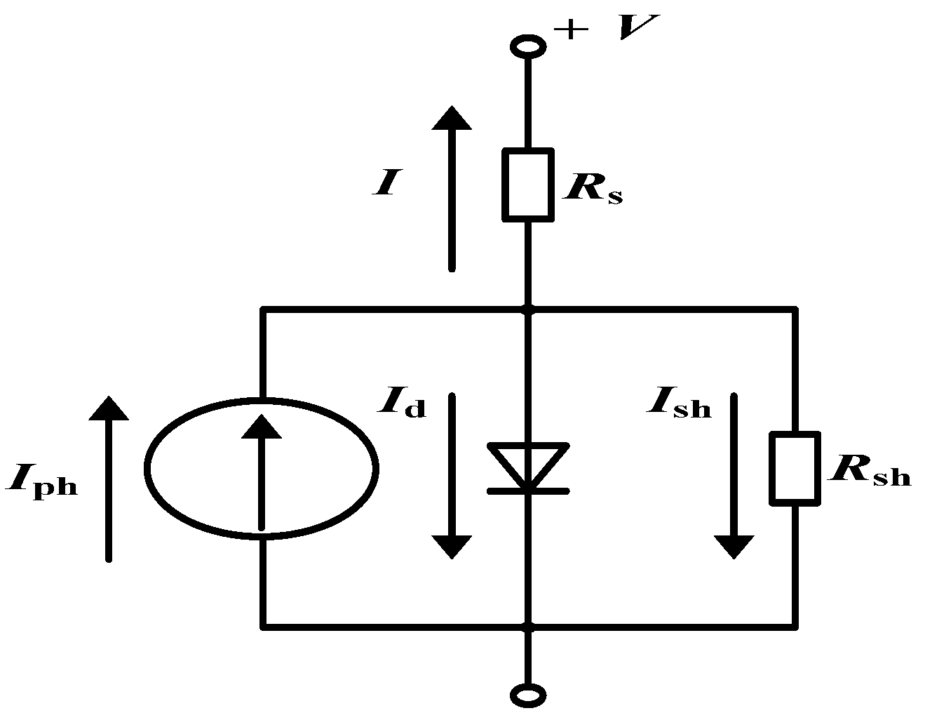
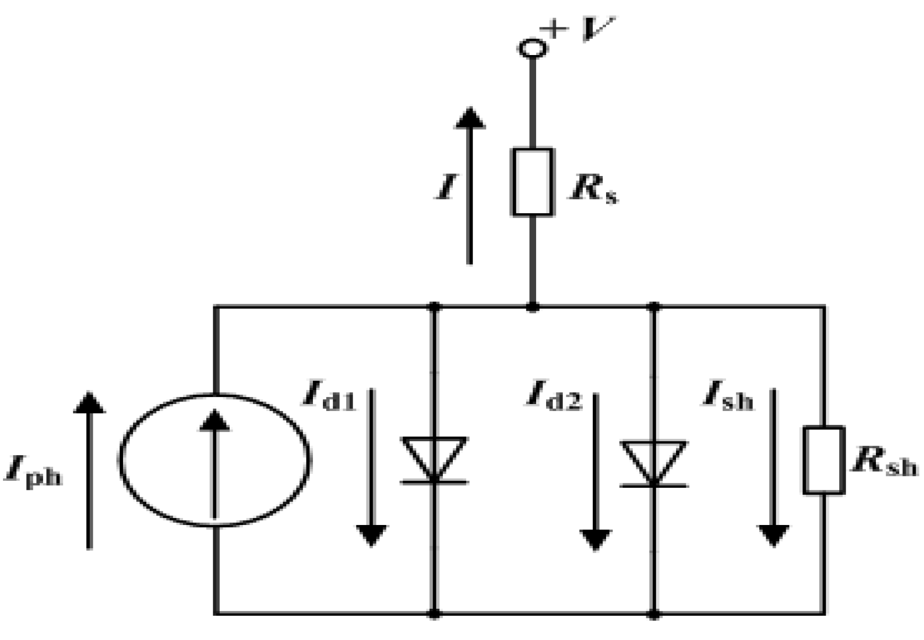
4.2. Parameter Identifications and Results
In order to prove the performance of the proposed method, it has been tested using the
I-
V characteristic of a 57 mm diameter commercial silicon solar cell [
17,
18]. The experimental data has been collected from the system under one sun (1000 W/m
2) in standard test conditions.
Table 4 reports experimental values of voltage and current. The experiment presents the results of five different algorithms when they are employed to identify the cell parameters considering the single and double diode models. For parameter identification, the control parameters for IABC, ABC, DE and PSO are the same as those in
Table 2. In addition, the control parameters artificial bee swarm optimization (ABSO) in [
19] is the same with those in [
19] as given by Equation (17). During the optimization process, the objective function is minimized with respect to the parameters’ range. The upper and lower bounds of the parameters are shown in
Table 5. The identified parameters are employed to reconstruct the
I-
V characteristic. The relative error
e(
t) in Equation (17) is used to further confirm the accuracy of the identified model.
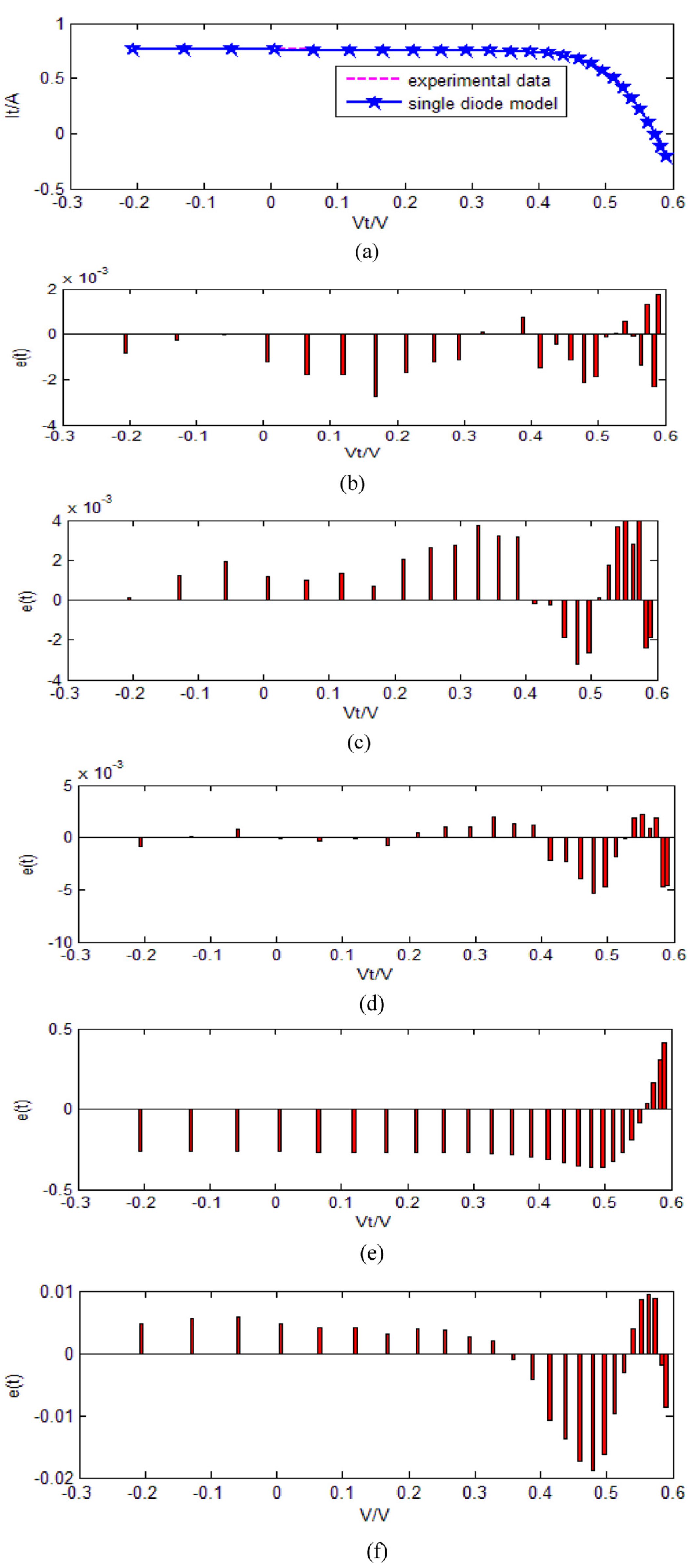
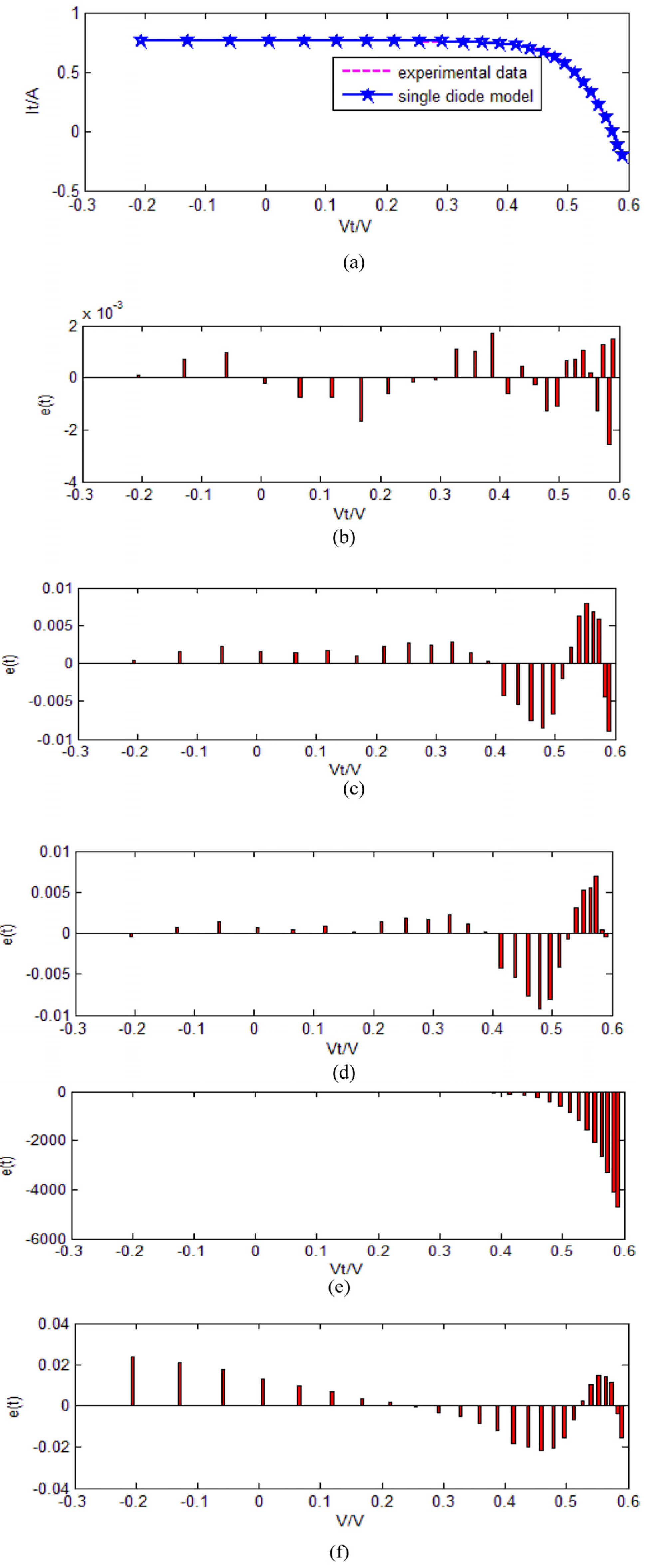
Figure 6 and
Figure 7 illustrate the results comparison of four methods for both the single and the double diode models.
where
Ic(
t) is a current calculated by the respective model. The smaller
e(
t) is, the higher accuracy the identified model demonstrates.
Table 4.
Terminal I-V measurements.
Table 4.
Terminal I-V measurements.
| Measurement | Measured V | Measured I |
|---|
| 1 | −0.2057 | 0.7640 |
| 2 | −0.1291 | 0.7620 |
| 3 | −0.0588 | 0.7605 |
| 4 | 0.0057 | 0.7605 |
| 5 | 0.0646 | 0.7600 |
| 6 | 0.1185 | 0.7590 |
| 7 | 0.1678 | 0.7590 |
| 8 | 0.2132 | 0.7570 |
| 9 | 0.2545 | 0.7555 |
| 10 | 0.2924 | 0.7540 |
| 11 | 0.3269 | 0.7505 |
| 12 | 0.3585 | 0.7465 |
| 13 | 0.3873 | 0.7385 |
| 14 | 0.4137 | 0.7280 |
| 15 | 0.4373 | 0.7065 |
| 16 | 0.4590 | 0.6755 |
| 17 | 0.4784 | 0.6320 |
| 18 | 0.4960 | 0.5730 |
| 19 | 0.5119 | 0.4990 |
| 20 | 0.5265 | 0.4130 |
| 21 | 0.5398 | 0.3165 |
| 22 | 0.5521 | 0.2120 |
| 23 | 0.5633 | 0.1035 |
| 24 | 0.5736 | −0.0100 |
| 25 | 0.5833 | −0.1230 |
| 26 | 0.5900 | −0.2100 |
Table 5.
Upper and lower range of the solar cell parameters.
Table 5.
Upper and lower range of the solar cell parameters.
| Parameters | Lower | Upper |
|---|
| Rs/Ω | 0 | 0.5 |
| Rsh/Ω | 0 | 100 |
| Iph/A | 0 | 1 |
| IL, IL1, IL2/A | 0 | 1 |
| a, a1, a2 | 1 | 2 |
Figure 6 and
Figure 7 are the average of 20 independent experiments.
Figure 6a and
Figure 7a indicate that the
I-
V characteristic found by IABC is in good agreement with the experimental data. The smaller
e(
t) value in
Figure 6 and
Figure 7 mean that our proposed method provides better accuracy. Comparing the proposed method outcomes with other methods results in the above experiments, the proposed method clearly outperformed other competing methods.
Figure 6.
The comparison of the results of four methods for the single diode model: (a) comparison between the I-V characteristics generated using our proposed method and the measured data; (b) relative error for each measured value based on the identified parameters using IABC algorithm; (c) relative error for each measured value based on the identified parameters using ABC algorithm; (d) relative error for each measured value based on the identified parameters using DE algorithm; (e) relative error for each measured value based on the identified parameters using PSO algorithm; (f) relative error for each measured value based on the identified parameters using ABSO algorithm.
Figure 7.
The comparison of the results of four methods for the double diode model: (a) comparison between the I-V characteristics generated using our proposed method and the measured data; (b) relative error for each measured value based on the identified parameters using IABC algorithm; (c) relative error for each measured value based on the identified parameters using ABC algorithm; (d) relative error for each measured value based on the identified parameters using DE algorithm; (e) relative error for each measured value based on the identified parameters using PSO algorithm; (f) relative error for each measured value based on the identified parameters using ABSO algorithm.
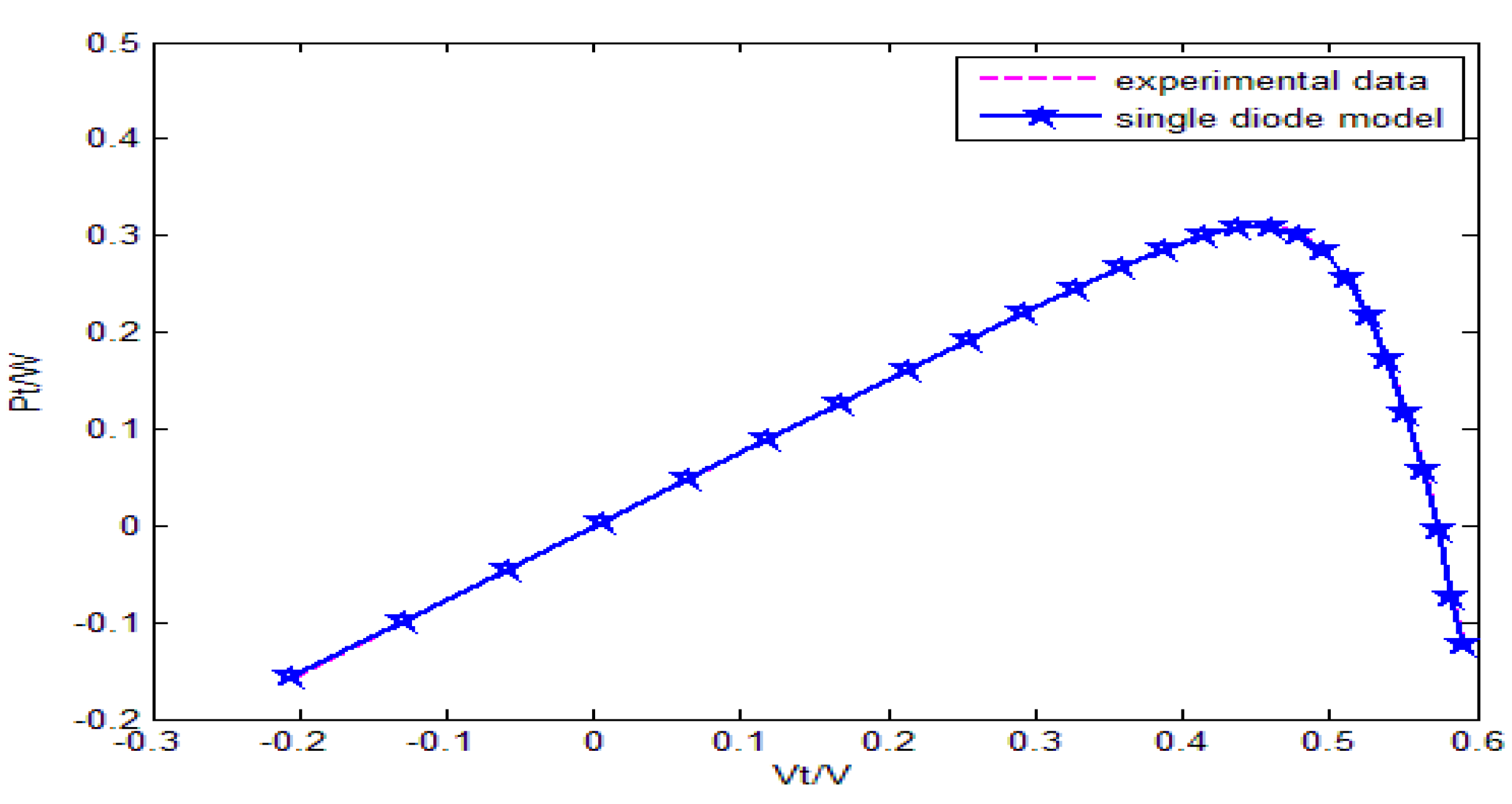
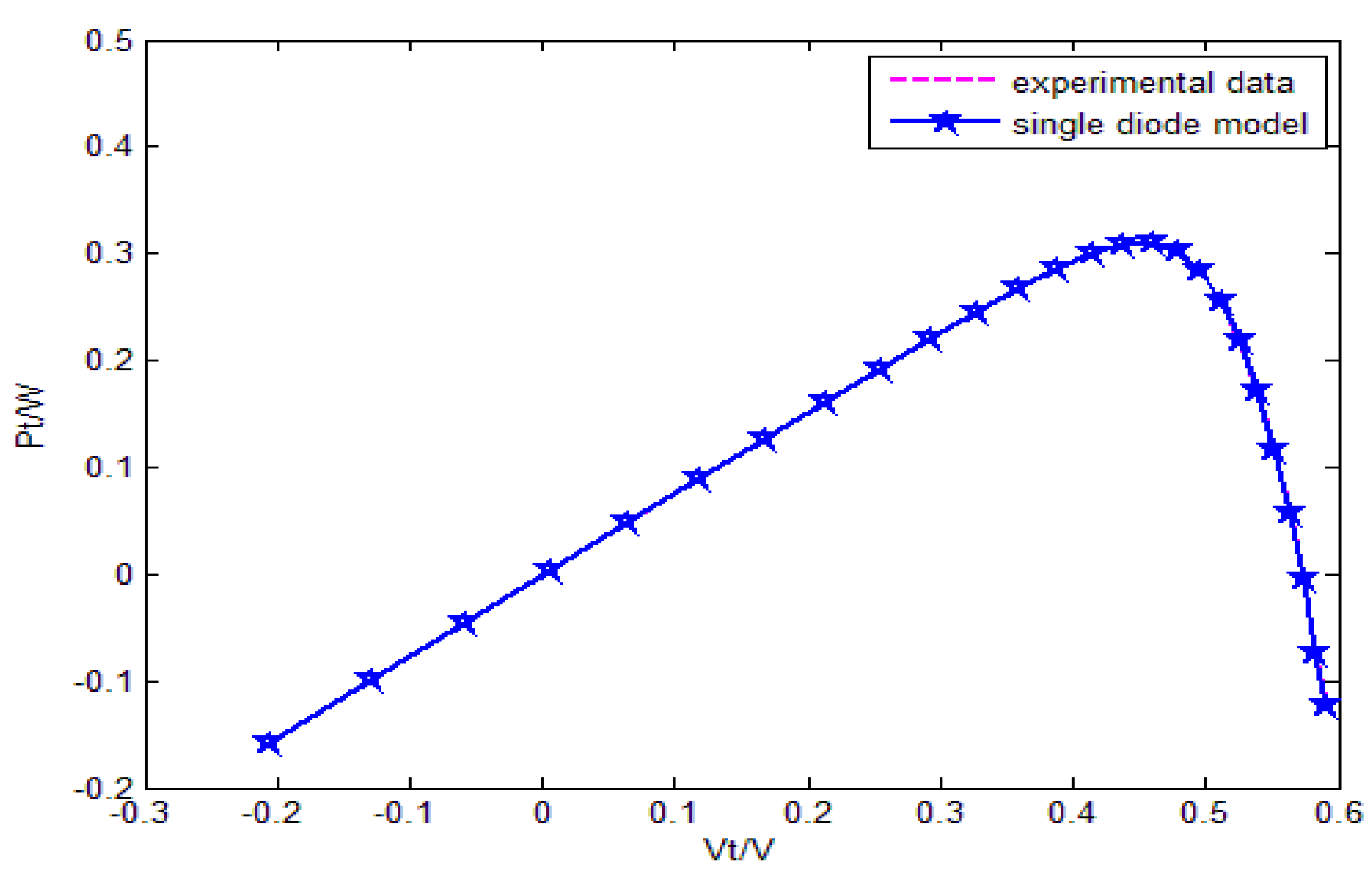
To further investigate the quality of the identified parameters, we put them into the power
vs. voltage (
P-
V) characteristic which is reconstructed. The
P-
V characteristic resulted from the identified model along experimental data is shown in
Figure 8 and
Figure 9, respectively. The similarity between the model results and the performance of the real system proves the superiority of the proposed method.
Figure 8.
Comparison between the P-V characteristics resulting from the experimental data and the single diode model.
Figure 8.
Comparison between the P-V characteristics resulting from the experimental data and the single diode model.
Figure 9.
Comparison between the P-V characteristics resulting from the experimental data and the double diode model.
Figure 9.
Comparison between the P-V characteristics resulting from the experimental data and the double diode model.
Recently, a deterministic approach was used to solve the problem of parameter identification for solar cells, such as [
5,
6,
20],
etc. Firstly, the comparison between the proposed method, the method in [
20] (see 2.D) and the method in [
5] is made in terms of computational cost. The computational cost of the proposed method is as follows:
times additional and/or subtraction operation for single diode model,
times additional and/or subtraction operation for double diode model, and
times multiplication and/or division operation for single diode model,
times multiplication and/or division operation for double diode model, note that
nstep is the number of function evaluations. The computational cost of the method in [
20] (see 2.D) is as follows:
times additional and/or subtraction operation, and
times multiplication and/or division operation. Here
is the evaluation number which determines the initial value of
Rs and
a. The computational cost of the method in [
5] is as follows:
times additional and/or subtraction operation, and
times multiplication and/or division operation, and
times integration operation. In the standard condition, the optimal parameter value of three different methods is summarized in
Table 6. The
nstep of the proposed method are 603 and 932 for the single and double diode models, respectively. The
nstep of the proposed in [
5] is 23 while the
nGuess and
nstep of the method in [
20] are 147 and 178. Note that the value of
nGuess and
nstep are different from [
20] because we and [
20] chose different initial values for the independent parameters
Rs and
a.
Table 6.
Identified parameters after applying different methods.
Table 6.
Identified parameters after applying different methods.
| Parameters | The Proposed Method | The Method in [20] | The Method in [5] |
|---|
| Single Diode Model | Double Diode Model |
|---|
| Rs/Ω | 0.0363 | 0.0364 | 0.0365 | 0.0364 |
| Rsh/Ω | 54.4610 | 55.2307 | 52.8591 | 53.7804 |
| Iph/A | 0.7599 | 0.7609 | 0.7609 | 0.7608 |
| IL (or IL1)/A | 3.3243 × 10⁻⁷ | 2.6900 × 10⁻⁷ | 0.3102 | 0.0407 |
| IL2/A | - | 2.8198 × 10⁻⁷ | - | 0.2874 |
| a (or a1) | 1.4842 | 1.4670 | 0.0390 | 1.4495 |
| a2 | - | 1.8722 | - | 1.4885 |
| J(θ) | 0.0010 | 0.0010 | 9.8126 × 10⁻⁴ | 0.0011 |
In the subsequence, we made a comparison between the proposed method, the method in [
20] (see 2.D) and the method in [
5] by conducting an experiment under nonstandard test conditions. The
Rmse index defined by Equation (19) is used to measure accuracy of different methods. The experiment results of one diode model was summarized in
Table 7, while the experiment results of two diode models was summarized in
Table 8.
Table 7.
Results obtained by different methods for the single diode model in nonstandard test conditions.
Table 7.
Results obtained by different methods for the single diode model in nonstandard test conditions.
| Testing Temperature | Methods |
|---|
| The Method in [20] | The Proposed Method |
|---|
| 25 °C | 9.8126 × 10⁻⁴ | 0.0010 |
| 50 °C | 9.8126 × 10⁻⁴ | 0.0010 |
| 75 °C | 9.8126 × 10⁻⁴ | 0.0010 |
| 100 °C | 5.8605 × 10⁻³ | 0.0010 |
Table 8.
Results obtained by different methods for the double diode model in nonstandard test conditions.
Table 8.
Results obtained by different methods for the double diode model in nonstandard test conditions.
| Testing Temperature | Methods |
|---|
| The Method in [5] | The Proposed Method |
|---|
| 25 °C | 9.9191 × 10⁻⁴ | 0.0010 |
| 50 °C | 2.7984 × 10⁻³ | 0.0010 |
| 75 °C | 4.6523 × 10⁻³ | 0.0010 |
| 100 °C | 3.5554 × 10⁻³ | 0.0010 |
The result comparison for single diode model is shown in
Table 7. The
Rmse is relatively low, which also implies higher accuracy among experiments. The
Rmse of the proposed method is slightly bigger than the result of the method in [
20] at
T = 25 °C,
T = 50 °C and
T = 75 °C, and only smaller than the result of the method in [
20] at
T = 100 °C. From the results comparison shown in
Table 7, the method in [
20] yields the better result in terms of
Rmse than the proposed method in some cases. In general, [
20] has benefit in that they utilize reduced forms to decrease the dimension of the parameter space. The method in [
5] further reduces the dimension of the parameter space to one. However, the method in [
5] usually returns precise results only when a high number of points on the
I-
V curve are available. It may be why the
Rmse of the proposed method is smaller than the result of the method in [
5] shown in
Table 8. The method in [
20] has deficiencies: (1) a different solution can be achieved if different reduced forms are used; (2) not directly applicable to multi-diode model parameter identification due to the limitation of Lambert W function formalism. The ABC algorithm is very suitable for the search for a global optimal solution, such as model parameter identification of solar cells in this paper. Unique solutions are achieved if the algorithm converges to the same value, so the first drawback of [
20] can be avoided. It can also be used for the multiple-diode model.
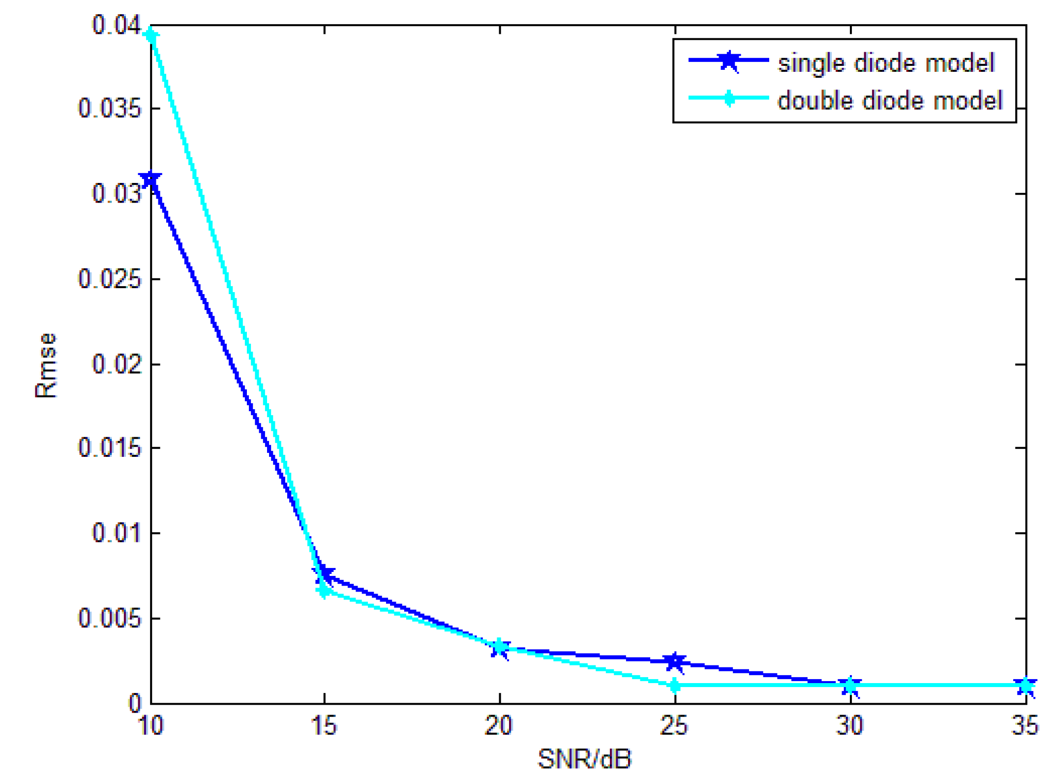
To examine the noise impacts for the distinct performance of the proposed method, in the last experiment, the measured data
V is added with varied white Gaussian noise of varying SNR (signal to noise ratio, SNR) from 10 to 35 dB. Moreover, we compared the single diode model with the double diode model. The estimate performance is evaluated by Equation (19).
Figure 10 shows the comparison of results of two models.
Figure 10.
Robustness of the two different models against noise.
Figure 10.
Robustness of the two different models against noise.
According to the result in
Figure 10, the single diode model demonstrates a better performance for noise robustness than the double diode model when SNR is below 15 dB. However, the double diode model displays better performance for noise robustness than the single diode model when SNR exceeds 15 dB.


