1. Literature Review
As an environmentally friendly sustainable energy, wind speed has become the fastest-growing new energy source and accordingly is increasingly getting widespread attention [
1,
2,
3]. In 2013, the newly increased total installed global wind power capacity was 35 GW, of which China accounted for 45.9%. Wind power represented approximately 2.5% of the country’s total generating capacity in 2013. With the implementation of wind power development policies, the number of single unit wind generator sets and the total generating capacity of large grid-connected wind farms are growing rapidly, and the impact on the power system is becoming more and more obvious. In view of this, a lots of research has been put forward in the area of wind power prediction. According to the characteristic curve of a wind generator, the output power can be calculated from the wind speed, so the accurate prediction of wind speed is in high demand.
In recent years, scholars have published important work on wind speed forecasting. The most used methods can be classified as time series modeling and intelligent algorithm modeling. Most of these methods are based on time series analysis, including vector autoregressive (VAR) models [
4] and autoregressive moving average (ARMA) models [
5,
6,
7,
8]. Erdem [
5] performed forecasting of wind speed and direction tuples based on ARMA; after the decomposition of wind speed, an ARMA model was proposed to represent each component and the results were combined to obtain the wind direction and speed forecasts. Wu [
6] introduced a new class of model which removed the restriction that the roots of AR and MA polynomials were outside the unit circle and established consistency and asymptotic normality of the least absolute deviation estimator under a non-Gaussian setting. Liu [
7] evaluated the effectiveness of ARMA-GARCH approaches, and successfully applied the proposed model in simulating the mean and volatility of wind speed and effectively caught the trend change of the wind speed. Jiang [
8] proposed a hybrid model based on ARMA. Through judgement of conditional heteroskedasticity of a generalized autoregressive function, this paper validates the advantages of the proposed model for wind speed prediction. Although time series modeling establishes linear or non-linear mapping relations of the historical wind speed to forecast the future speed by extracting information contained in the historical signals, it is criticized by researchers for its non-linear fitting capability weakness.
In order to deal with wind speed forecasting, intelligent algorithm modeling builds a high dimension non-linear function to fit the historical wind speed data, such as artificial neural networks (ANN) [
9,
10,
11,
12,
13] and LSSVM [
14,
15,
16,
17]. De Giorgi [
14] executed a comparative study of wind speed prediction. In their study, LSSVM with Wavelet Decomposition (WT) were evaluated and compared to hybrid ANN-based models at different time ranges. The root mean square error criterion was used to compare the accuracy of the different models. Liu [
15] developed a new wind speed forecasting strategy based on LSSVM and empirical mode decomposition (EMD). Two steps were put forward by the authors to make predictions: (a) the wind speed time was decomposed by EMD; (b) the LSSVM model was established to forecast each IMF. In [
16], Shuai put forward a LSSVM model and built an intellectual prediction model with multi-input variables. The optimal parameters of LSSVM were selected automatically, which obviously improved the speed and accuracy of the forecasting. Wang [
17] investigated LSSVM-based wind speed prediction with the consideration of power characteristics, unit efficiency and generator operation.
The regularization parameter γ and kernel parameter σ
2 have a great impact on LSSVM performance. Inappropriate selection of regularization parameter and kernel parameter values may make the LSSVM prediction model vulnerable to over-fitting and under-fitting problems. For this problem, hybrid models are promoted to achieve better overall system results [
18,
19,
20,
21,
22]. Sun [
18] studied LSSVM optimized by particle swarm optimization (PSO) and carried out a confirmation test by taking some wind farm data measured in Inner Mongolia as the example. Xu [
19] used PSO to improve the forecasting performance of LSSVM. Their study results validated that the hybrid PSO-LSSVM algorithm has better forecasting performance than single LSSVM algorithms. Song [
21] designed a new hybrid wind speed prediction approach by combing harmony search (HS) and LSSVM. In this method, a HS algorithm was employed to realize the adaptive selection of the regularization parameter γ, kernel function parameter σ
2, and a novel fusion algorithm. From the literature we know that due to the poor ability of PSO in the optimization process, it is easy to fall into a local optimum in LSSVM regularization parameter selection. Although HS algorithm has strong capability in global exploration and convergence, its weak local searching ability may lead to slow convergence speed at a later time. In order to overcome these drawbacks and for better clarity, in 2010, BA was proposed by Yang as an effective way to search for the global optimal solution [
22]. Under appropriate conditions, this algorithm can be considered a hybrid algorithm combing the HS algorithm and PSO algorithm. Preliminary studies [
23,
24,
25,
26] indicated that the BA is better to HS and PSO for solving unconstrained optimization problems and it was successfully applied with excellent selection results. Yammani (2014) [
23] exploited a BA based strategy for the dis tributed generation with renewable bus available limit constraint. Kang [
24] performed an experiment comparing the binary BA with other dimensionality reduction approaches. Experimental results showed that the proposed methodology was superior to other dimensionality reduction approaches. Rao [
25] developed an optimal power flow with generation reallocation using the BA. Because of the excellent performance of the BA in parameter optimization, in this paper, BA was used to select and automatically adjust appropriate parameters in the LSSVM model.
When forecasting wind speed with different models, the original data is usually used directly as independent variables. However, due to the chaotic nature and inherent complexity of wind speed, describing the movement trends of wind speed and accurately predicting it become difficult. In order to construct a suitable prediction model, it is very necessary to analyze the original data features. Thus, the multi-scale decomposition of the original wind speed, which is indispensable in improving the prediction accuracy, is widely used. Wavelet transform (WT) is used to eliminate the irregular fluctuation of the weed speed [
27,
28]. Liu [
27] described a wind speed forecasting method based on spectral clustering (SC), echo state networks (ESNs) and WT which was used to decompose the wind speed into multiple series to eliminate irregular fluctuation. Mandal [
28] described a hybrid intelligent algorithm that used a data preprocessing model based on WT and a soft computing model (SCM) based on neural network (NN). WT was applied to decompose the original wind speed data. The SCM and NN were used to forecast the decomposed wind speed data. Another method, empirical mode decomposition (EMD) is also applied to decompose the wind speed into several intrinsic mode functions (IMFs) for modeling [
29,
30]. Hong [
29] came up with a novel method based on the integration of EMD with ANN. EMD was presented to improve the ability of the standard ANN model to cope with the volatility and intermittency of wind speeds. From the presented literature review, it can be seen that the selection of a particular base wavelet and scale level may cause a false wave in WT decomposition while EMD has good self-adaptability and stable decomposition results in dealing with nonlinear and non-to address this shortcoming, ensemble empirical mode decomposition (EEMD) was proposed by Huang in 2009 [
31]. Compared with EMD, EEMD has good performance in non-stationary signal decomposition. To further enhance the real-time computational performance of EEMD, in 2014 Wang presented a new decomposition algorithm which was named fast ensemble empirical mode decomposition (FEEMD) [
32]. In our study, the latest FEEMD is used to convert the origin wind data into multiple empirical modes and its results are included in the comparison with EMD and WT.
Most wind speed forecasting methodologies discussed above used signal decomposition or parameter selection to improve the modeling accuracy, and few of them take the input selection into consideration. Thus, in this paper, a hybrid forecasting model is built with consideration of the input selection. In order to choose a proper input, not only Cointegration and Granger causality tests [
33] are exploited to select the proper environmental factors, but PACF is also proposed to calculate the wind speed lags.
This paper proposes a hybrid model which based on FEEMD-BA-LSSVM for wind speed forecasting. The paper is organized as follows:
Section 2 provides the a brief description of FEEMD, BA and LSSVM;
Section 3 presents the framework of the proposed technique;
Section 4 analyzes an experiment study to validate the proposed method;
Section 5 provides an additional forecasting experiment and
Section 6 concludes this paper.
3. FEEMD-BA-LSSVM Approaches
In this section, wind speed forecasting models incorporating FEEMD, BA and LSSVM are constructed as shown in
Figure 1 and
Figure 2.
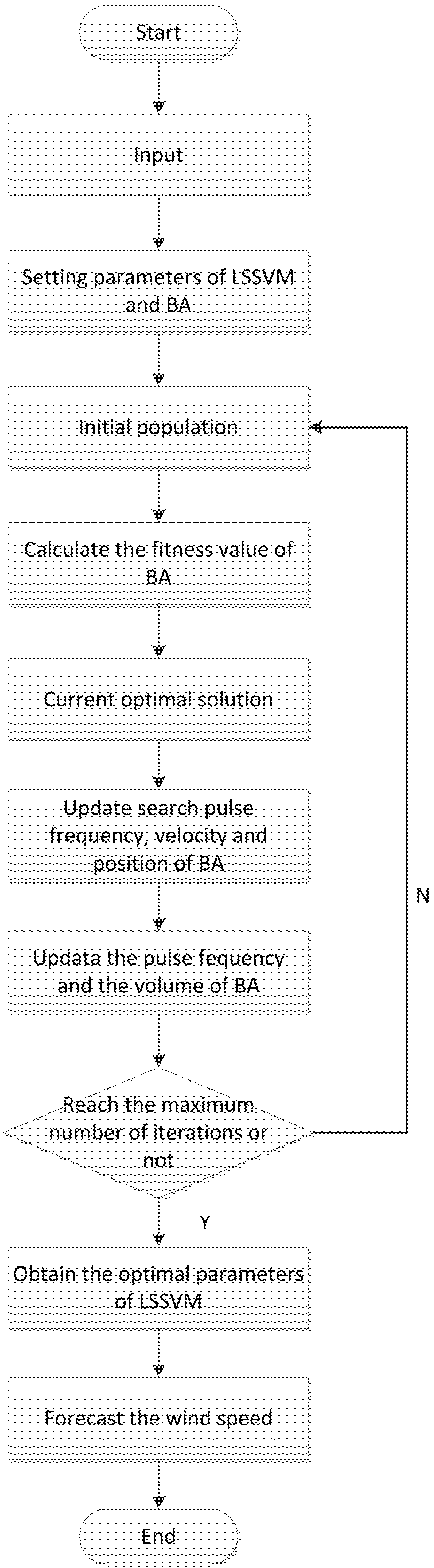
Figure 1.
The flowchart of BA-LSSVM.
Figure 1.
The flowchart of BA-LSSVM.
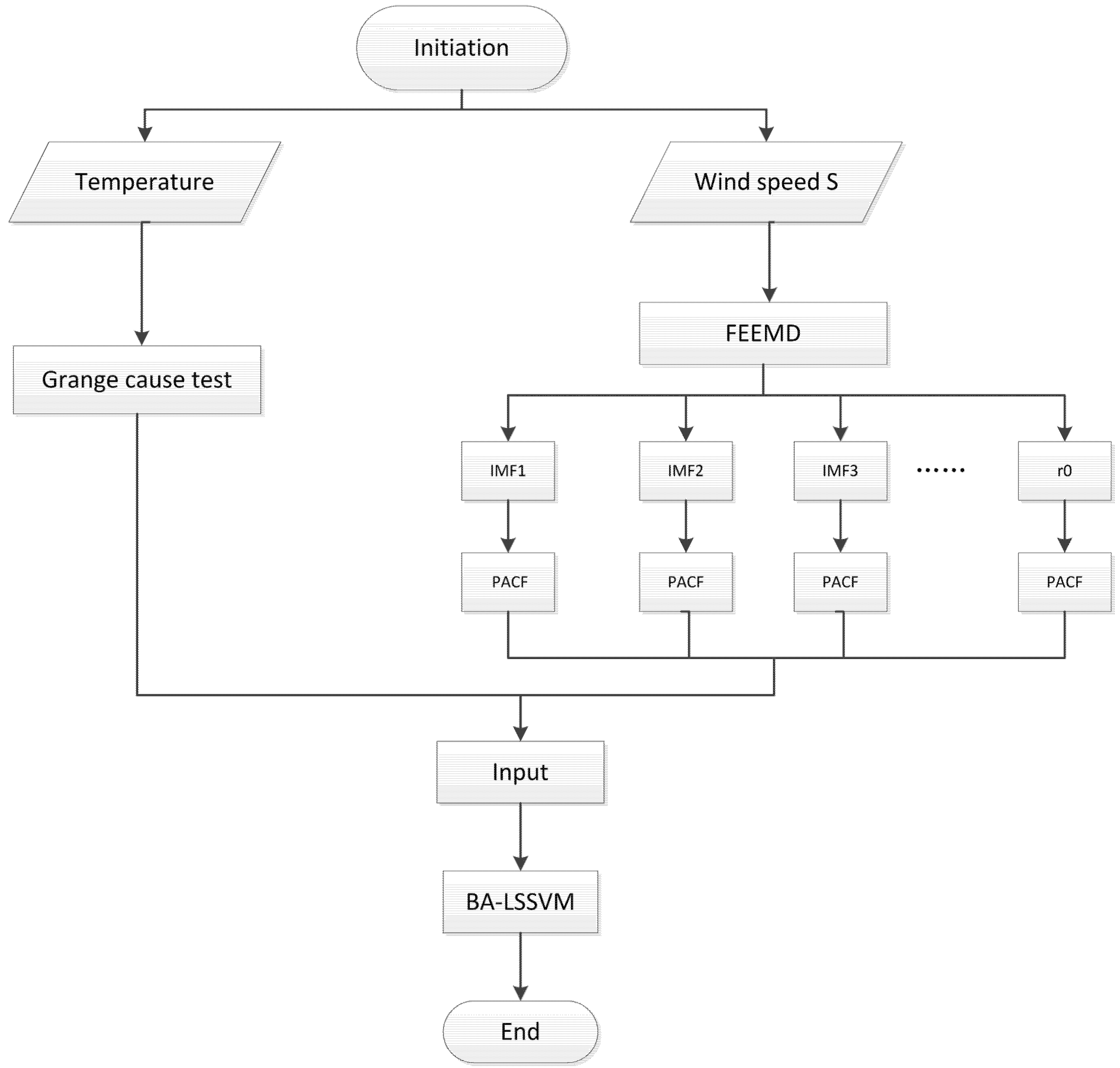
Figure 2.
The overall flowchart of FEEMD-BA-LSSVM.
Figure 2.
The overall flowchart of FEEMD-BA-LSSVM.
Based on the BA-LSSVM model, the combinatory optimization of parameters can be obtained as follows:
- (1)
Initialization parameters
The main parameters of BA algorithm are initial population size n, initial volume A, pulse rate r, position vector x and speed vector v. We determine the range of bat frequency f and the initial position xi.
- (2)
Population initialization
Initialize bat populations location, each bat position solution is a component by the γ and σ.
Based on the merits of the fitness value, find the current optimal solution, and update bat pulse frequency, speed and location as follows:
where,
represents uniformly distributed random numbers;
is the search pulse frequency of bat i,
;
and
represents the speed of bat I at time t and t-1, respectively, while
and
represents the position of bat I at time t and t-1.
is the current optimal solution for all bats.
- (4)
Update pulse frequency and volume
Generate uniformly distributed random number rand, if the rand > r
i, randomly disturb the optimal solution and produce a new solution, if rand <A
i while
, then the new solution is accepted and r
i and A
i are update as follows:
- (5)
Output the optimal solution
Sort all bat fitness values and find out the current optimal solution. Repeat steps (2) to (4) up to the maximum number of iterations. Output the global optimal solution, according to the optimal parameters, and establish the wind speed forecasting model.
The BA-LSSVM algorithm flowchart is shown as
Figure 1.
Figure 2 shows the overall process of FEEMD-BA-LSSVM. The modeling flowchart contains three steps. Prior to constructing the models, FEEMD is used to decompose the wind speed S into a finite number of IMFs, where each IMFs prominently feature different local data characteristics. Thus the decomposition can accurately grasp the characteristics of the original information.
This paper selects temperature, which belongs to the weather variables, in different periods as an exogenous wind speed variable using a Granger causality test and historical wind speeds as endogenous variables by calculating PACF. After FEEMD pretreatment and the selection of input, the original wind data are divided into the training set and the test set.
In the second step, LSSVM is proposed to model the sub-series in the first part, respectively, so that the tendencies of the sub-series can be predicted. The training error is averaged and used as a fitness function of BA, and then BA is used to optimize a group of parameters of LSSVM to minimize the fitness value. The final forecast is obtained by summing the forecasts for the various series obtained from FEEMD. Finally, LSSVM with optimal parameters which are obtained by the BA are used to forecast the wind speed.
4. Case Studies
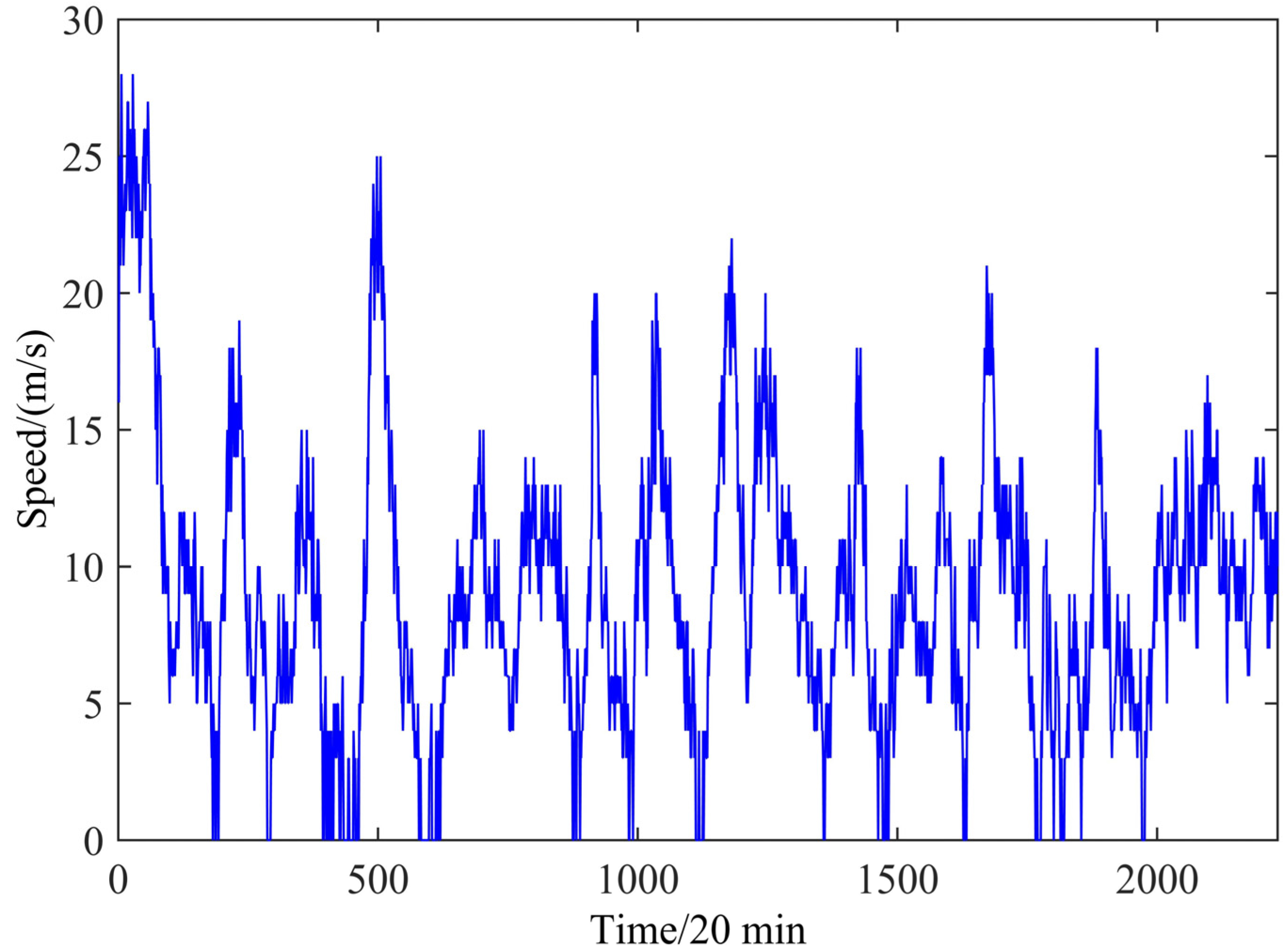
Inner Mongolia, a vast territory, is rich in wind resources, which are mainly distributed in the typical steppe, desert steppe and desert areas. The region’s technically exploitable wind energy resources can be developed to provide about 50% of the total wind energy resources in China, thus ranking first in the country. For our simulation the short-term wind speed data for the Rose Camp wind farm in Inner Mongolia, China are obtained every 20 min from 1 January 2011 to 3 February 3 2011. Data points (2232) recorded between 1 January 2011 and 31 January 2011 are selected as training samples, and data from 1 February to 3 February are selected as test samples. The altitude of the wind speed is 43 m.
Figure 3 shows the wind speed of the 2232 January data points. The figure shows that the wind speed fluctuates severely, ranging from 0 m/s to nearly 30 m/s. From the figure, we cannot see any apparent regularity in the wind speed.
Figure 3.
Wind speed during the period from 1 January to 31 January 2011.
Figure 3.
Wind speed during the period from 1 January to 31 January 2011.
4.1. Statistical Measures to Determine the Accuracy of the Forecast
Three criteria—mean absolute error (MAE), mean absolute percentage error (MAPE) and root mean square error (RMSE)—are applied to quantitatively examine the proposed model performance:
where n represents the number of the speeds to be forecasted,
.
is the t-th actual speed and
is the forecast wind speed at the same point. Through literature study, we know that MAPE of the wind speed ranges from 25% to 40% [
34], which is related to the models used in forecasting as well as the forecasting horizon and local wind characteristics. In a normal state, forecasting horizon and wind speed accuracy are closely related, and the shorter the forecasting horizon is or more stable the wind speed is, the smaller the forecasting error will be, and on the contrary, the forecasting error will be larger [
35].
4.2. Input Selection for Short-Term Wind Speed Forecasting
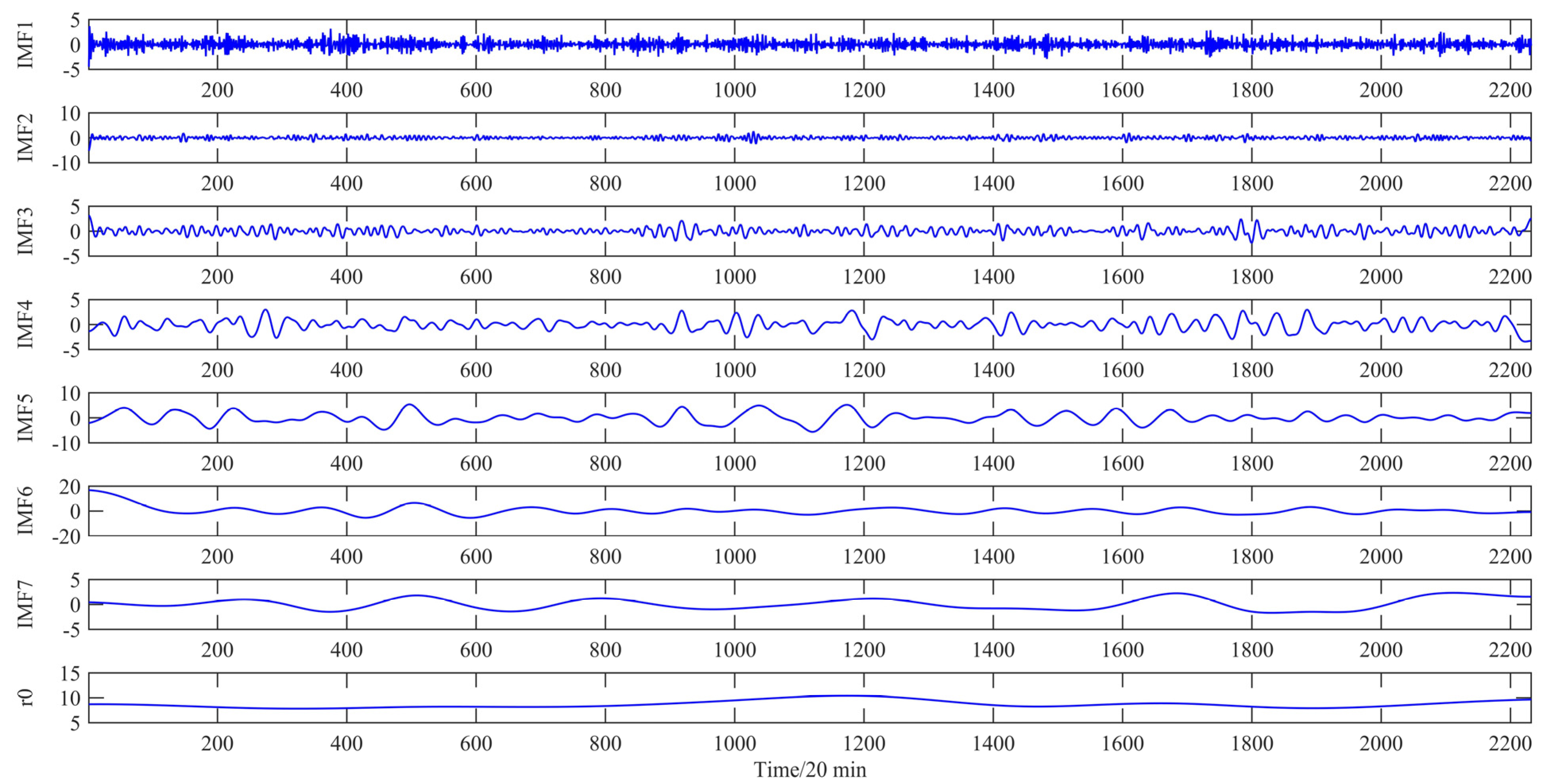
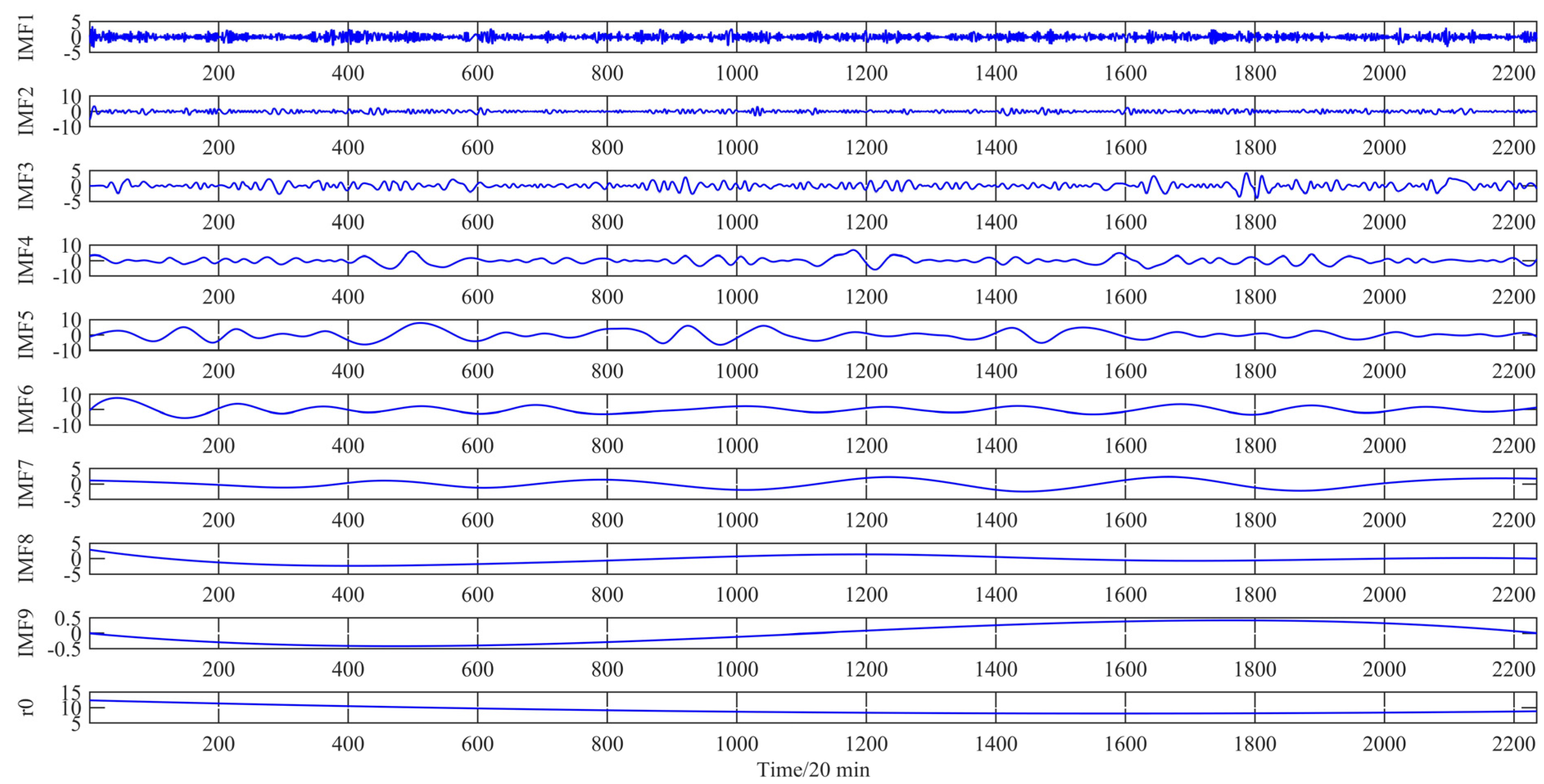
FEEMD is adopted to decompose the original series to eliminate the stochastic volatility for the next step. As a result, seven independent IMFs and one residue are shown in
Figure 4.
Figure 4.
The decomposition of the wind speed during the period from 1 January to 31 January 2011 by FEEMD.
Figure 4.
The decomposition of the wind speed during the period from 1 January to 31 January 2011 by FEEMD.
This paper aims at investigating the performance of the proposed models. For comparison EMD and WT are applied for decomposing the original wind speed data. EMD is similar to FEEMD, and the results is shown in
Figure 5. From
Figure 5, the wind speed is decomposed into eight IMFs and one residue.
Figure 5.
The decomposition of the wind speed during the period from 1 January to 31 January 2011 by EMD.
Figure 5.
The decomposition of the wind speed during the period from 1 January to 31 January 2011 by EMD.
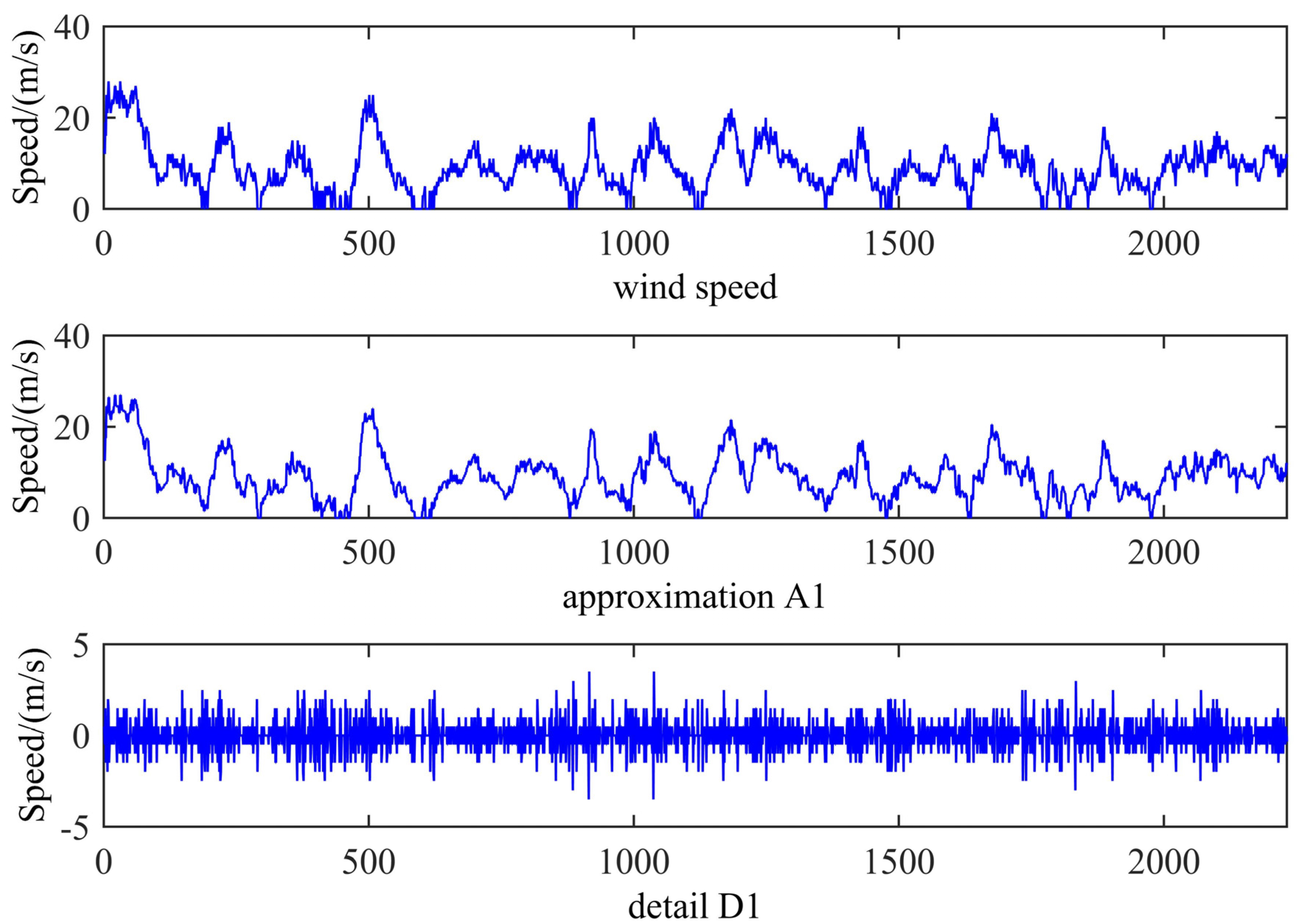
WT is exploited to decompose the original wind speed data into an approximation component A
1 and a detail component D
1 as shown in
Figure 6. As can be seen from
Figure 6, A
1 shows high similarity to the original wind speed data, presenting major fluctuations of wind speed while other minor irregularities appear in D
1, so A
1 is taken as the wind speed to model for accuracy.
In this paper, a LSSVM model will be built to forecast the wind speed in the following sections. As previously described, the performance of LSSVM mainly depends on the selection of input and parameters, so here, we labor to select the input by using a Granger causality test and partial autocorrelation analysis.
Figure 6.
The decomposition of the wind speed during the period from 1 January to 31 January 2011 by WT.
Figure 6.
The decomposition of the wind speed during the period from 1 January to 31 January 2011 by WT.
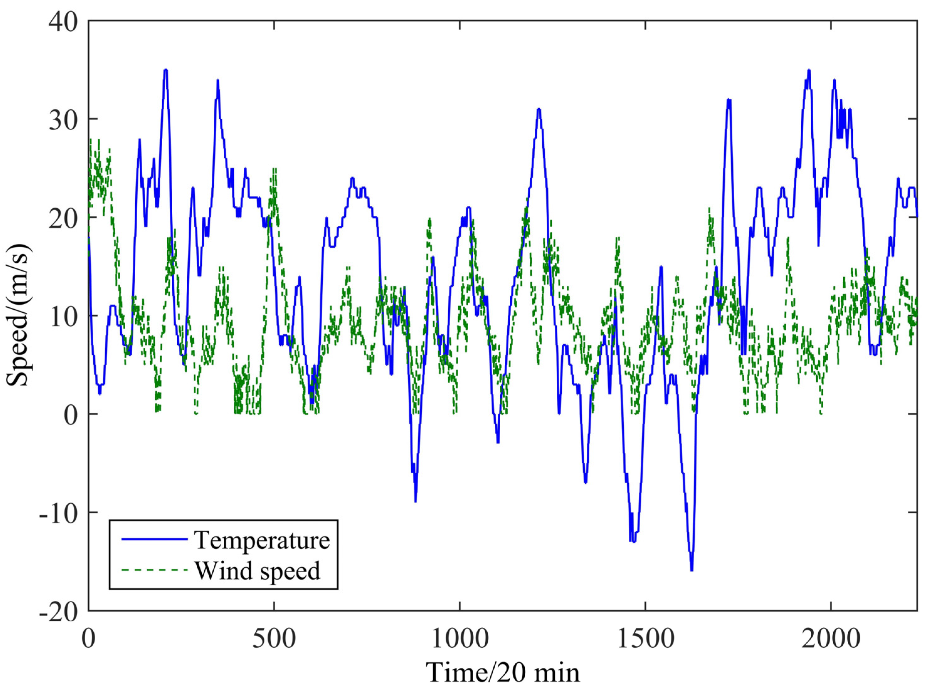
In order to mine the environmental information, the correlation between temperature and wind speed is analyzed.
Figure 7, which shows 2232 samples of wind speed and the corresponding temperatures, shows that the wind speed fluctuation lags behind the corresponding temperature.
Thus, the Granger causality test is applied to analyze the exact dependence of the two variables with different lags. This test method was pioneered by the 2003 Nobel Laureate in Economics, Clive W.J. Granger. The Granger causality test was originally used to analyze the relationship between economic variables. The precondition for the Granger causality test is that time series must be stationary, or this may cause spurious regression problems and therefore the Granger causality test is invalid and distorted for non-stationary variables. However, in reality, time series is generally non-stationary. It can be made stable but then we lose the long-term information of the total amount which is necessary for signal analysis, so a Cointegration test is proposed to resolve this problem.
Figure 7.
Relationship between the wind speed and temperature.
Figure 7.
Relationship between the wind speed and temperature.
The Cointegration test considers whether there is a long-term stable relationship in non-stationary variables and if there is any, the regression is not a spurious regression. This paper applies Eviews 7.0 (QMS Company, Boca Raton, FL, USA) under Windows 7 system to perform a Johansen and Juselius Cointegration test, whose results are shown in
Table 1 and
Table 2.
Table 1.
Unrestricted Cointegration Rank Test.
Table 1.
Unrestricted Cointegration Rank Test.
| Hypothesized | Eigenvalue | Trace | 0.005 | Prob. ** |
|---|
| No. of CE(s) | Statistic | Critical Value |
|---|
| None * | 0.011 | 23.825 | 21.751 | 0.002 |
| At most 1 | 5.34 × 10⁻⁵ | 0.106 | 7.879 | 0.744 |
Table 2.
Unrestricted Cointegration Rank Test (Maximum Eigenvalue).
Table 2.
Unrestricted Cointegration Rank Test (Maximum Eigenvalue).
| Hypothesized | Eigenvalue | Max-Eigen | 0.005 | Prob. ** |
|---|
| No. of CE(s) | Statistic | Critical Value |
|---|
| None * | 0.011 | 23.719 | 20.267 | 0.001 |
| At most 1 | 5.34 × 10⁻⁵ | 0.106 | 7.879 | 0.744 |
According to the Cointegration test, wind speed and the corresponding temperature have a long-term stable relationship, thus a Granger causality test can be carried out.
Table 3 shows the Granger causality test results from Lag 1 to Lag 4 for wind speed and the corresponding temperature.
Table 3.
Probability to reject in Granger causality test between wind speed and temperature.
Table 3.
Probability to reject in Granger causality test between wind speed and temperature.
| Supposition | Lag 1 | Lag2 | Lag3 | Lag4 |
|---|
| Wind speed does not cause temperature | 0.6079 | 0.3734 | 0.2527 | 0.1912 |
| Temperature does not cause wind speed | 0.0257 | 0.0011 | 0.0067 | 0.0379 |
As it is shown in
Table 3, Lag 2 and Lag 3 the supposition of “Temperature does not cause wind speed” are under the significance level of 0.005. Lag 2 shows the minimum value, illustrating that temperature affects wind speed lagged 2 and 3. Thus, the temperature 2 ahead is chosen as the environmental variable for LSSVM input with the historical wind speed. However, the information that “Wind speed does not cause temperature” has less relationship with the accuracy of wind speed forecasting, so this paper will not discuss the analysis of this results.
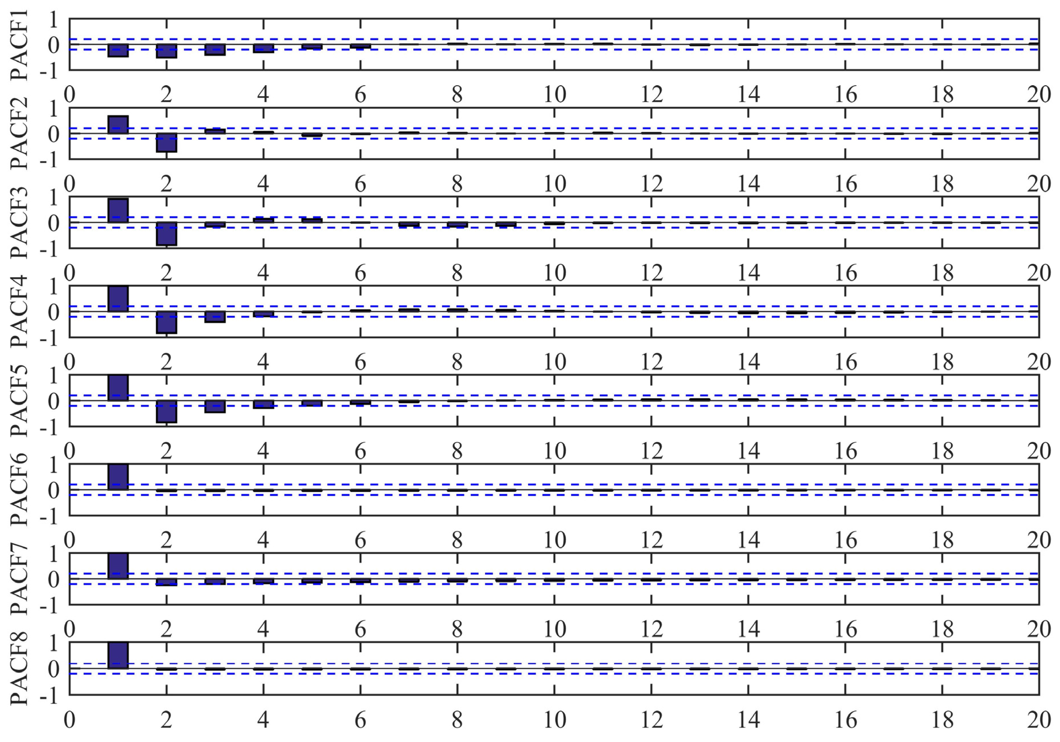
After FEEMD, the partial correlation analysis of the IMFs and the residue are applied to select the input of LSSVM which has the highest correlation with the forecast data.
Figure 8 is the plot of partial correlation analysis of the wind speed where PACF1~PACF7 stand for IMFs respectively and PACF8 represents the residue. Setting x
i as the output variable, if the PACF at lag k is out of the 95% confidence interval, x
i−k is applied as one of the input variables, so it is obvious that the input variables of these nine series for BA-LSSVM are the ones shown in
Table 4.
Figure 8.
The PACF of IMFs and one residue of the wind speed.
Figure 8.
The PACF of IMFs and one residue of the wind speed.
Table 4.
Result analysis of PACFs of IMFs and r0 of the wind speed after FEEMD.
Table 4.
Result analysis of PACFs of IMFs and r0 of the wind speed after FEEMD.
| IMFs and r0 | Lag |
|---|
| IMF1 | (xt−1,xt−2,xt−3,xt−4) |
| IMF2 | (xt−1,xt−2) |
| IMF3 | (xt−1,xt−2) |
| IMF4 | (xt−1,xt−2,xt−3) |
| IMF5 | (xt−1,xt−2,xt−3,xt−4) |
| IMF6 | (xt−1) |
| IMF7 | (xt−1,xt−2) |
| r0 | (xt−1) |
In the same way, the lags of PACF after EMD and WT are shown in
Table 5.
Table 5.
Result analysis of PACFs of the wind speed after EMD and WT.
Table 5.
Result analysis of PACFs of the wind speed after EMD and WT.
| EMD | WT |
|---|
| IMF1 | (xt−1,xt−2,xt−3,xt−4) | A1 | (xt−1,xt−2,xt−3) |
| IMF2 | (xt−1,xt−2,xt−3,xt−4,xt−5) |
| IMF3 | (xt−1,xt−2,xt−3,xt−4,xt−5, xt−6) |
| IMF4 | (xt−1,xt−2,xt−3,xt−4) |
| IMF5 | (xt−1,xt−2,xt−3,xt−4,xt−5) |
| IMF6 | (xt−1,xt−2,xt−3,xt−4) |
| IMF7 | (xt−1) |
| IMF8 | (xt−1,xt−2) |
| IMF9 | (xt−1,xt−2) |
| r0 | (xt−1) |
4.3. FEEMD-BA-LSSVM Result Analysis
As previously described, the performance of any LSSVM model relies on its parameters. BA is developed to adjust key LSSVM parameters by minimizing any errors generated in the training set. The LSSVM model is chosen as a basic model with RBF as the kernel function. Regularization parameter γ and kernel parameter σ
2 are tuned by BA automatically. The main parameters in BA modeling are listed in
Table 6. The regularization parameter γ and kernel parameter σ
2 of the LSSVM optimized by BA are 143.229 and 0.399, respectively.
Table 6.
Parameters of BA.
Table 6.
Parameters of BA.
| Main Parameters | Value | Main Parameters | Value |
|---|
| Initial population size | 10 | Initial volume | 0.25 |
| Pulse rate | 0.5 | Maximum frequency | 2 |
| Minimum frequency | 0 | Max- iteration number | 50 |
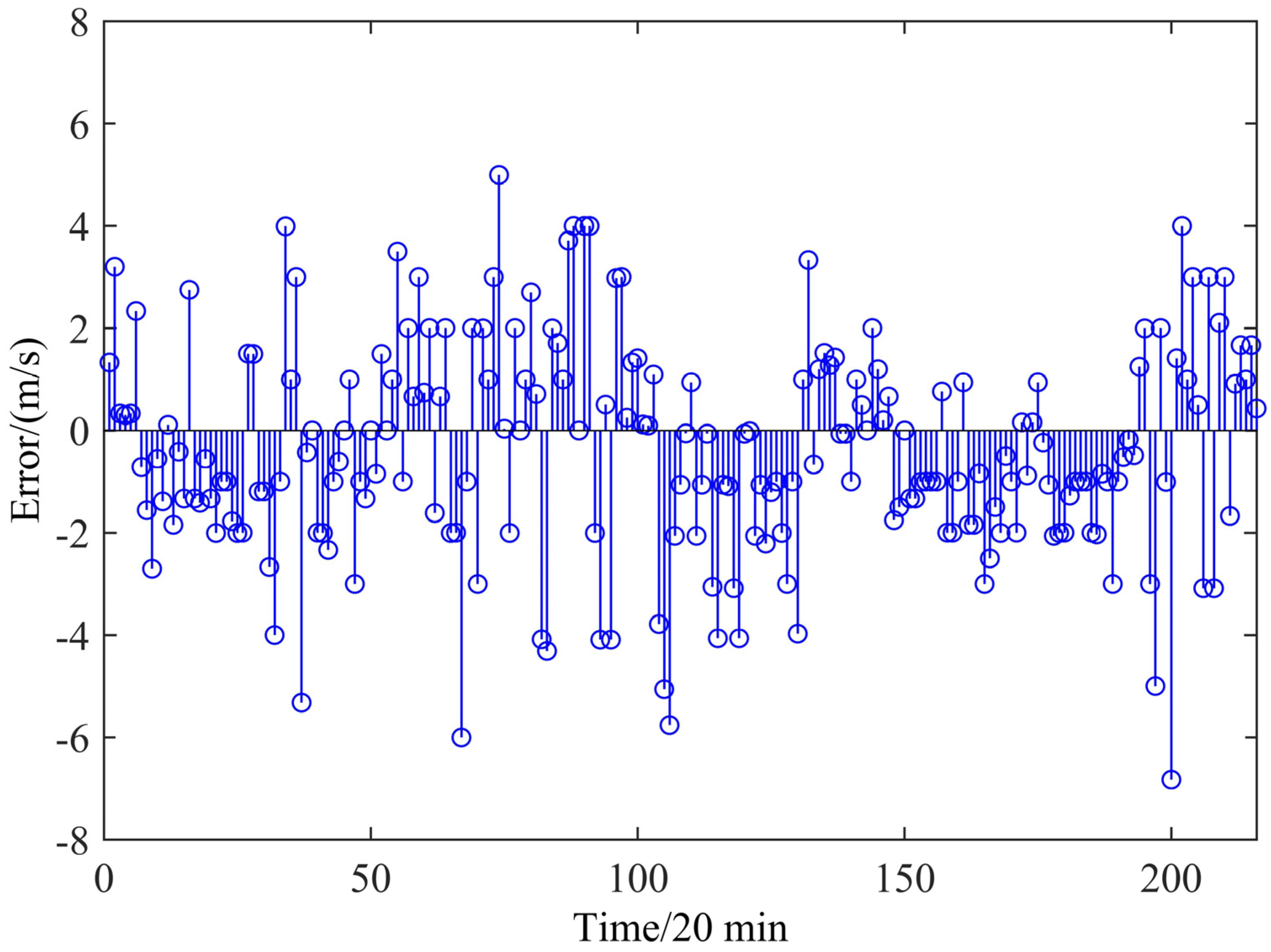
The test set is used to test the performance of the LSSVM model with the parameters selected by BA. In
Figure 9, the error by LSSVM is clearly shown. The error by LSSVM changes relatively stable and there is no large aggregation error in an interval. It can be seen that only four error points are out of 5 m/s and among them the maximum error only reaches −5.9997 which means that the prediction results can be accepted.
Figure 9.
The error of FEEMD-BA-LSSVM.
Figure 9.
The error of FEEMD-BA-LSSVM.
4.4. Comparative Analysis
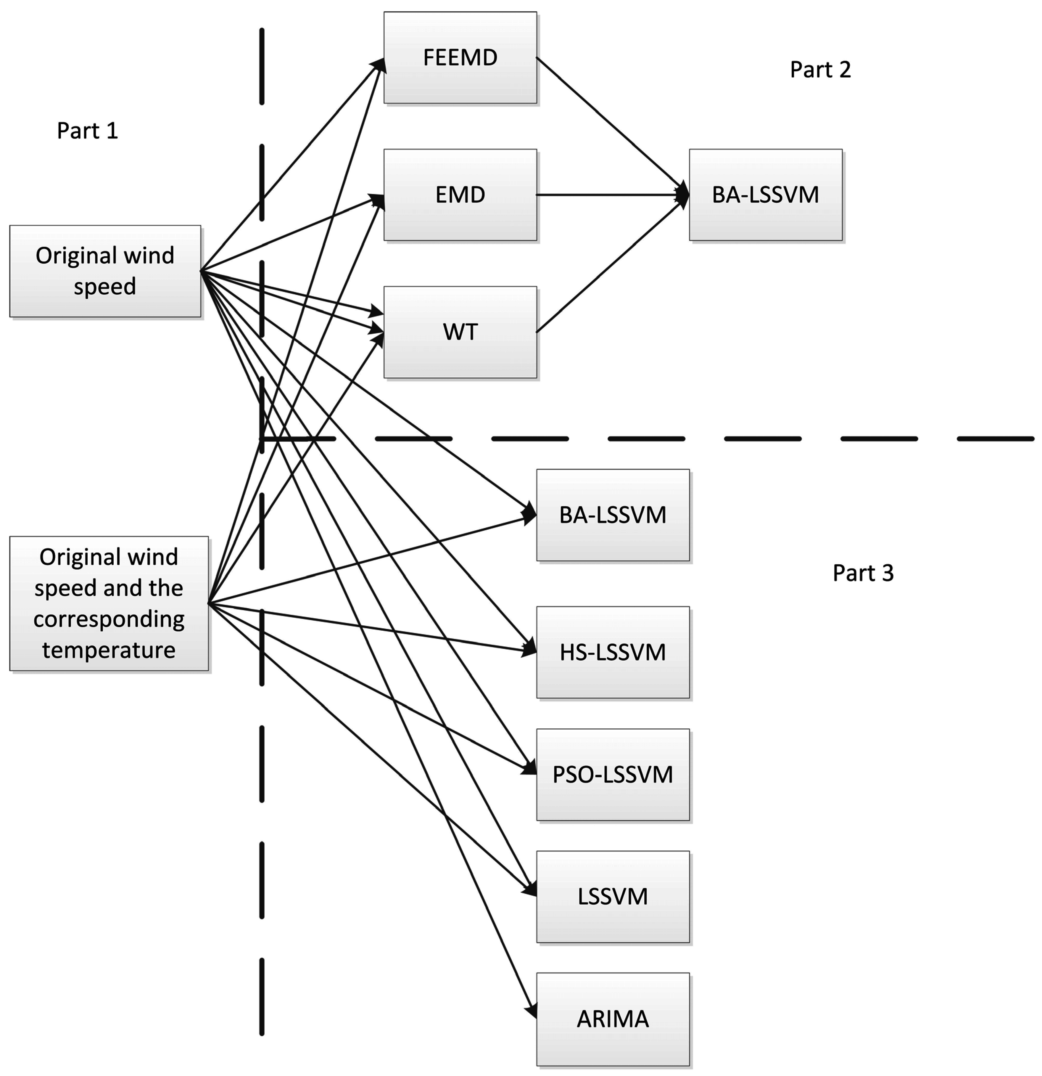
To demonstrate the advanced nature of the proposed method, in this study the framework of the comparative analysis is shown in
Figure 10. As shown in
Figure 10, the framework of the comparative analysis consists of three parts. From Part 1, as the paper proposes temperature as an independent variable in wind speed forecasting, the independent variables with and without temperature are applied in the same model to prove the correctness of introducing temperature as an argument.
In Part 2, three signal decomposition algorithms are adopted, which include the WT algorithm, EMD algorithm and FEEMD algorithm. Through the comparison between these algorithms, FEEMD, which is proposed in this paper, shows the best performance.
As shown in Part 3, different parameter selection algorithms are used to improve the performance of LSSVM, and further compared with single LSSVM and ARIMA. Among these forecasting models employed in the comparison, BA-LSSVM is the most accurate and perfect one in predicting the wind speed. Moreover, the prediction results of BA-LSSVM in Part 3 are also compared with Part 2 that verifies the necessity of filtering the original wind speed.
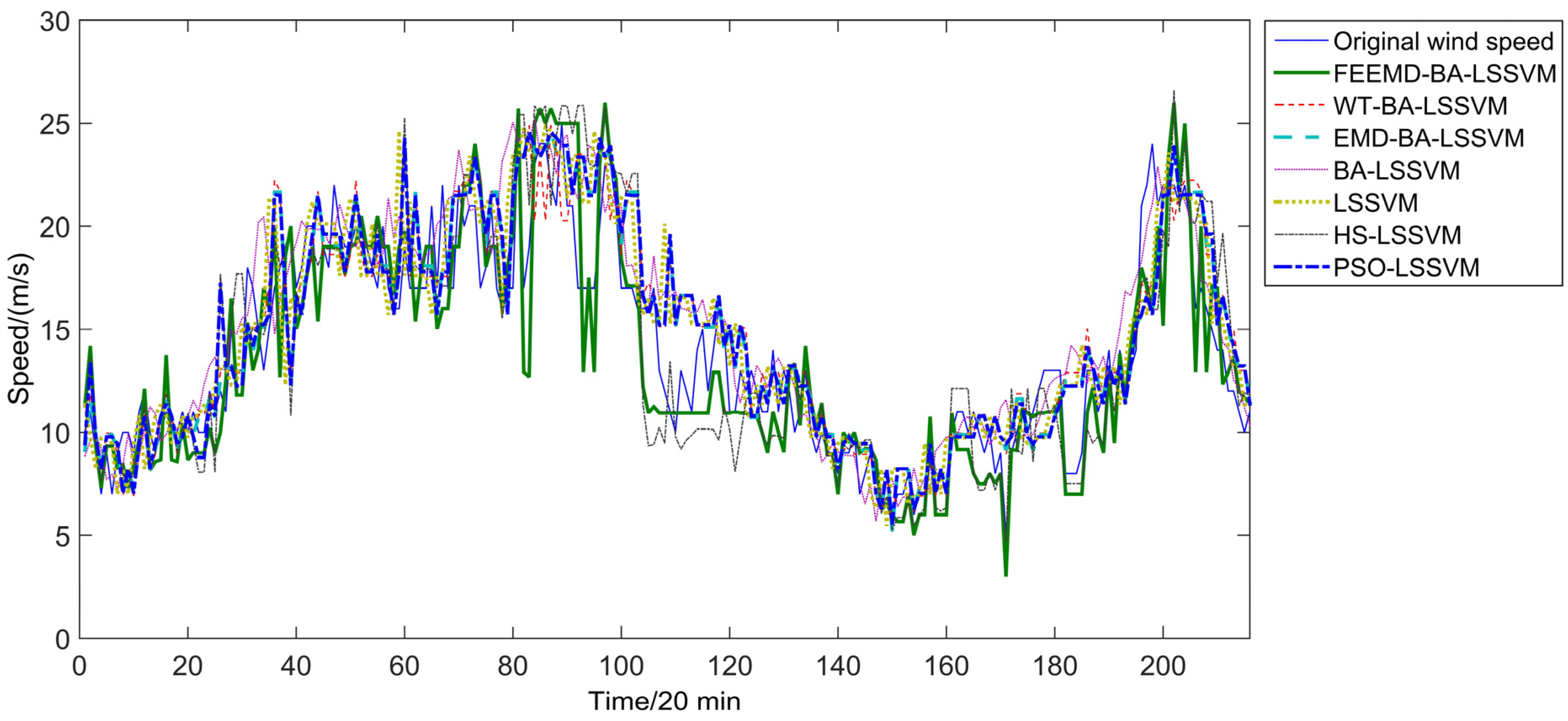
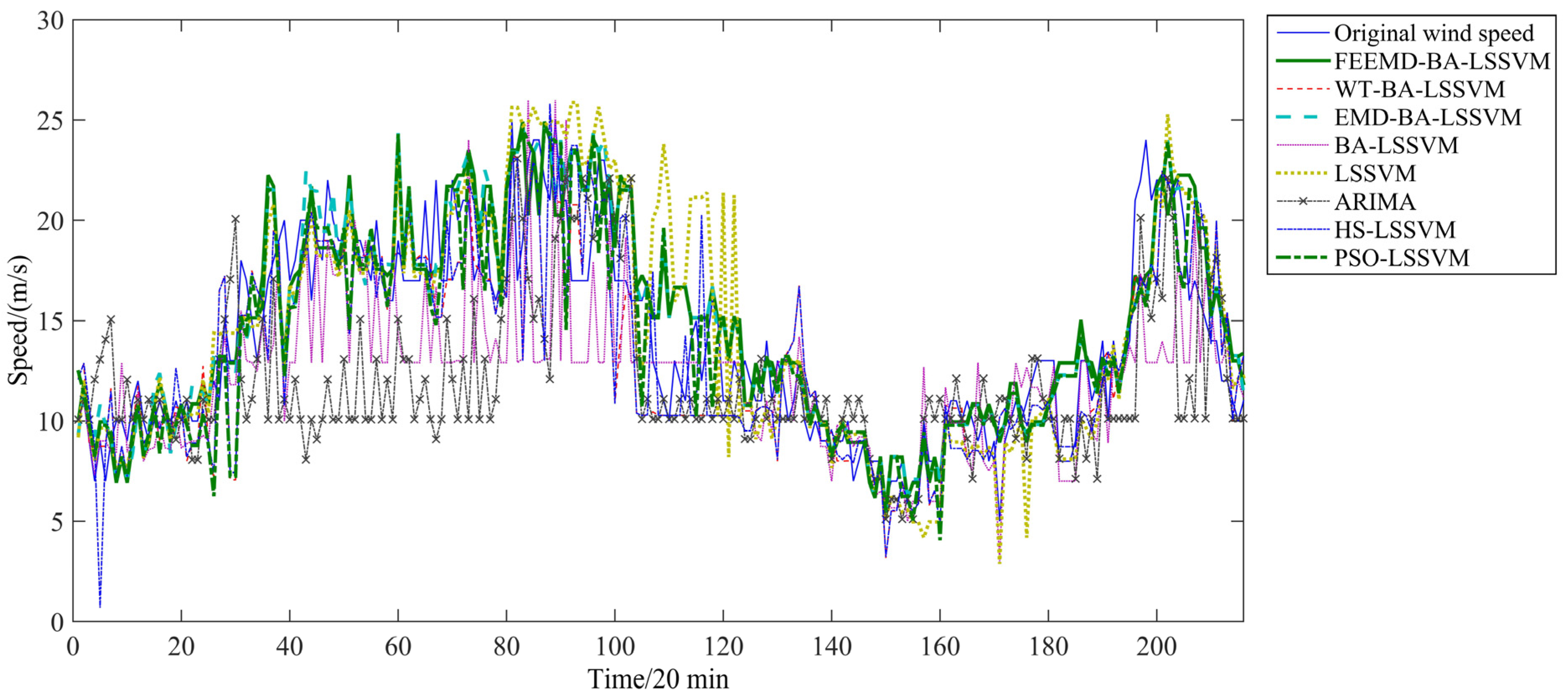
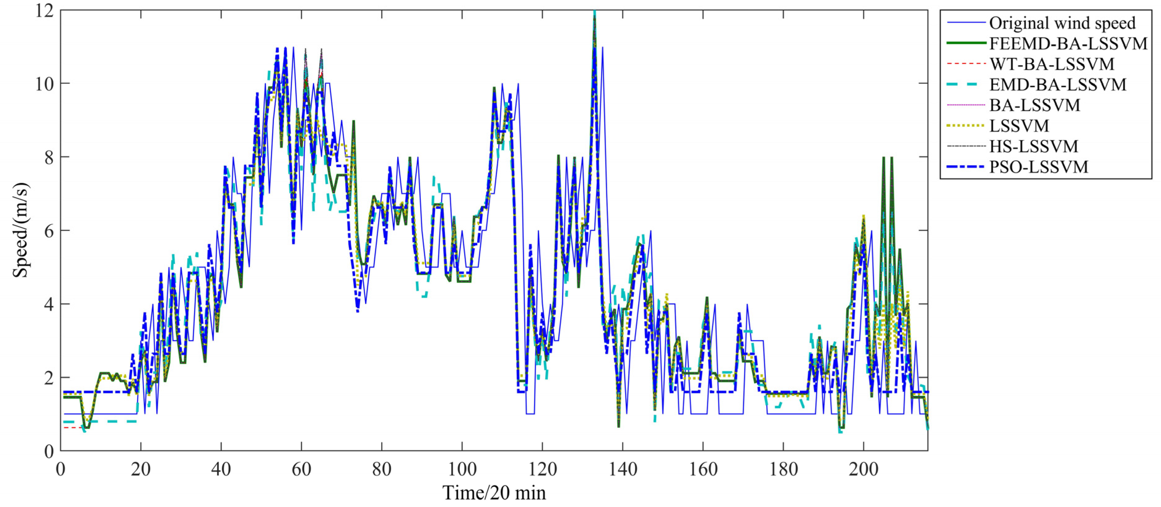
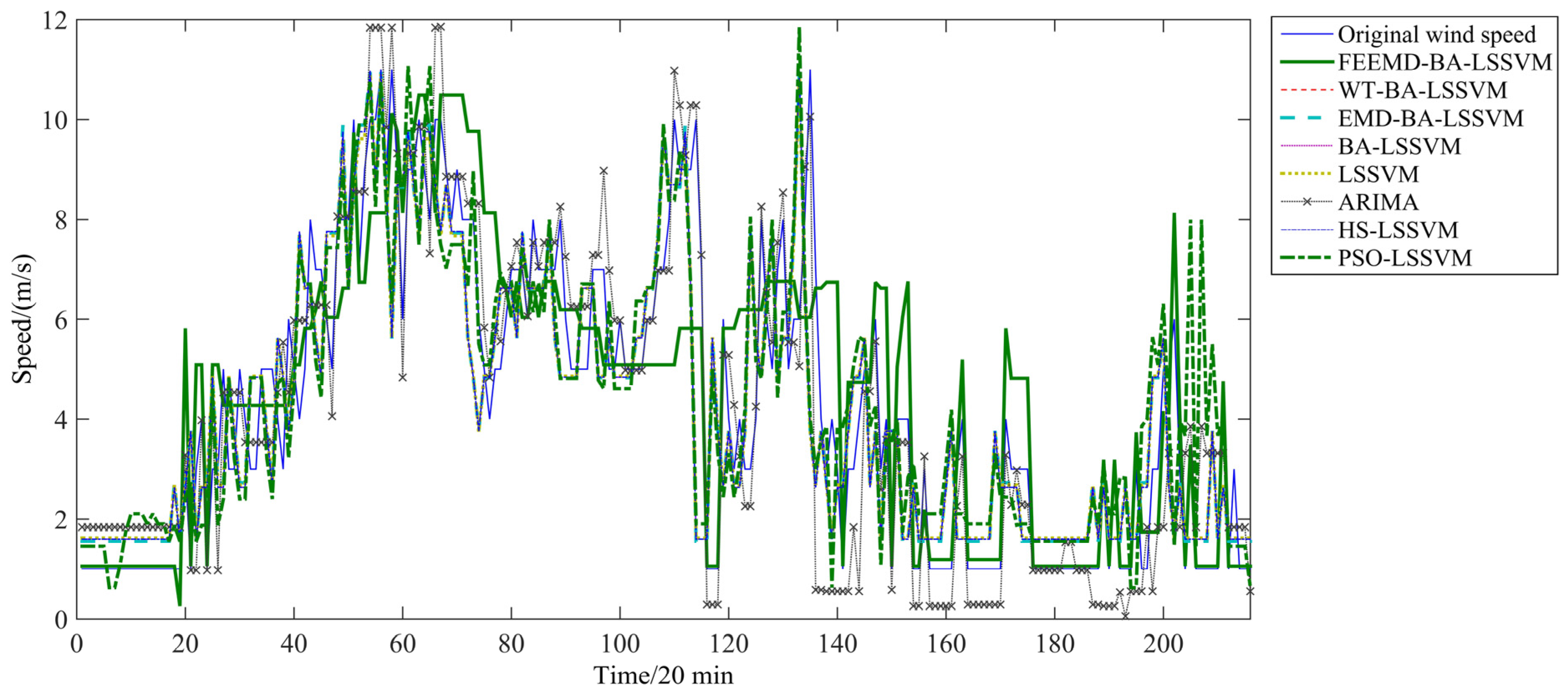
Figure 11 and
Figure 12 show the prediction results from February 1 to February 3 which contain 216 points by different models with the independent variables which include merely original wind speed or the original wind speed and the corresponding temperature. The estimated results of these predictions are given in
Table 7 and
Table 8.
Figure 10.
Framework of the comparative analysis.
Figure 10.
Framework of the comparative analysis.
Figure 11.
Forecasting results with temperature as argument.
Figure 11.
Forecasting results with temperature as argument.
Figure 12.
Forecasting results without temperature as argument.
Figure 12.
Forecasting results without temperature as argument.
Table 7.
Analysis of the predictions with temperature as argument.
Table 7.
Analysis of the predictions with temperature as argument.
| Indexes | Prediction Methods |
|---|
| | FEEMD-BA-LSSVM | WT-BA-LSSVM | EMD-BA-LSSVM |
| MAE (m/s) | 1.761 | 1.979 | 1.889 |
| MAPE (%) | 12.733 | 14.714 | 14.211 |
| RMSE (m/s) | 2.277 | 2.639 | 2.555 |
| | BA-LSSVM | HS-LSSVM | PSO-LSSVM |
| MAE (m/s) | 1.891 | 2.171 | 1.957 |
| MAPE (%) | 14.764 | 15.024 | 15.445 |
| RMSE (m/s) | 2.552 | 2.90 | 2.621 |
| | LSSVM | | |
| MAE (m/s) | 2.028 | | |
| MAPE (%) | 15.693 | | |
| RMSE (m/s) | 2.681 | | |
Table 8.
Analysis of the predictions without temperature as argument.
Table 8.
Analysis of the predictions without temperature as argument.
| Indexes | Prediction Methods |
|---|
| | FEEMD-BA-LSSVM | WT-BA-LSSVM | EMD-BA-LSSVM |
| MAE (m/s) | 1.981 | 2.111 | 2.017 |
| MAPE (%) | 14.771 | 15.305 | 15.076 |
| RMSE (m/s) | 2.641 | 2.802 | 2.638 |
| | BA-LSSVM | HS-LSSVM | PSO-LSSVM |
| MAE (m/s) | 2.330 | 2.576 | 2.348 |
| MAPE (%) | 16.665 | 17.156 | 17.162 |
| RMSE (m/s) | 2.966 | 3.560 | 3.050 |
| | LSSVM | ARIMA | |
| MAE (m/s) | 2.423 | 3.445 | |
| MAPE (%) | 18.008 | 22.965 | |
| RMSE (m/s) | 3.353 | 4.630 | |
From
Figure 11 and
Figure 12, the deviation between the actual value and the forecasting results for the eight forecasting models can be captured. In
Figure 12, the errors of ARIMA are almost higher than those of other forecasting models, which means it has poor performance on the testing set. FEEMD-BA-LSSVM gives acceptable predictions most of the time. Compared with the single LSSVM model, the improved LSSVM model is more suitable for wind speed forecasting. Furthermore, the proposed BA-LSSVM model shows better performance than other improved LSSVM models. The results prove that the parameters determined by the BA algorithm can efficiently improve the forecasting accuracy of the LSSVM. Moreover, the comparison between
Figure 11 and
Figure 12 shows that the forecasting results with temperature as argument are better on the whole than the forecasting results without temperature as argument using the same prediction methods.
From
Table 7 and
Table 8, it can be concluded that: (a) the introduction of the new argument significantly improves the prediction accuracy. All models in
Table 7 have higher accuracy than the ones in
Table 8, for example, FEEMD-BA-LSSVM’s MAPE in
Table 7 is 12.733% which is lower than the 14.771% of FEEMD-BA-LSSVM in
Table 8; (b) based on the MAE, MAPE and RMSE criteria, FEEMD-BA-LSSVM outperforms the BA-LSSVM which suggests that FEEMD helps to improve the performance of BA-LSSVM; (c) all the used decomposition models improve the forecasting performance of BA-LSSVM. In
Table 3, the MAPE of BA-LSSVM improved by FEEMD, WT and EMD is 12.733%, 14.714%, 14.211%, respectively. FEEMD has the best promoting performance and it retains its best position in
Table 8 while WT shows the poorest decomposition performance. The nature of WT is a Fourier transform with an adjustable window which cannot get rid of the limitations of the Fourier transform and is not suitable for solving nonlinear problems. What’s more, during the analysis, wavelet base and decomposition level require manual selection which causes a greater impact of subjective factors on the decomposition results. However, as a great breakthrough compared with the Fourier-based linear and stationary spectral analysis, EMD decomposes the time-series signal into a set of IMFs, rather than a sine or cosine function which is obtained through the Fourier transform. EMD can analyze not only linear stationary signals, but also perform non-linear non-stationary signal analysis. FEEMD improves on the basis of EMD, and effectively solves the mixing phenomenon of EMD and improves the computation speed. Thus, this method has the best decomposition results; (d) this paper builds three improved LSSVM models. Among them, the best performance belongs to BA-LSSVM, which produces better results than the other two models in terms of lower MAE, MAPE and RSME. This is because the PSO and HS algorithms are the special circumstances of simplified BA, and the BA algorithm combines the advantages of these algorithms. Besides, the MAE and RSME of HS-LSSVM model are slightly higher than those of the two counterparts, indicating that HS is more emphasis on MAPE while it ignores the other indexes if MAPE is taken as the sole fitness criterion; (e) all the improved LSSVM models are better than the single LSSVM model. A possible reason could be that the improved LSSVM model puts up with the auto-selection of parameters in LSSVM and has strong global search capability. It can be seen from
Table 8 that when comparing the single ARMA with all the LSSVM-based models, LSSVM-based models show better performance than the pure statistical ARMA. This proves that the intelligent models always have higher performance than the statistical models.
5. Case Two
To further investigate the performance of the proposed model, an additional case which selects wind speed data from 1 July 2010 to 31 July 2010 as training samples and 1 August 2010 to 3 August 2010 as test samples in the same place is provided in this study. The forecasting results of Case Two are presented in
Figure 13 and
Figure 14. The estimated results are demonstrated in
Table 9 and
Table 10.
Figure 13.
Forecasting results with temperature as argument.
Figure 13.
Forecasting results with temperature as argument.
Figure 14.
Forecasting results without temperature as argument.
Figure 14.
Forecasting results without temperature as argument.
From
Figure 13 to
Figure 14, the errors of ARIMA are still almost higher than those of the other forecasting models while FEEMD-BA-LSSVM still shows the best performance. The comparison between
Figure 13 and
Figure 14 shows that, with temperature as argument, the accuracy of prediction results obviously improves compared with the forecasting results without temperature as argument by same prediction methods.
Table 9.
Analysis of the predictions with temperature as argument.
Table 9.
Analysis of the predictions with temperature as argument.
| Indexes | Prediction Methods |
|---|
| FEEMD-BA-LSSVM | WT-BA-LSSVM | EMD-BA-LSSVM |
| MAE (m/s) | 1.714 | 1.900 | 1.849 |
| MAPE (%) | 11.057 | 14.496 | 14.246 |
| RMSE (m/s) | 2.167 | 2.792 | 2.697 |
| | BA-LSSVM | HS-LSSVM | PSO-LSSVM |
| MAE (m/s) | 1.958 | 2.171 | 1.935 |
| MAPE (%) | 15.193 | 15.498 | 15.508 |
| RMSE (m/s) | 2.813 | 2.961 | 2.973 |
| | LSSVM | | |
| MAE (m/s) | 2.319 | | |
| MAPE (%) | 16.293 | | |
| RMSE (m/s) | 2.988 | | |
Table 10.
Analysis of the predictions without temperature as argument.
Table 10.
Analysis of the predictions without temperature as argument.
| Indexes | Prediction methods |
|---|
| | FEEMD-BA-LSSVM | WT-BA-LSSVM | EMD-BA-LSSVM |
| MAE (m/s) | 1.978 | 2.345 | 1.991 |
| MAPE (%) | 14.430 | 15.661 | 14.498 |
| RMSE (m/s) | 2.631 | 2.813 | 2.665 |
| | BA-LSSVM | HS-LSSVM | PSO-LSSVM |
| MAE (m/s) | 2.351 | 2. 351 | 2. 345351 |
| MAPE (%) | 16.498 | 17.147 | 17.499 |
| RMSE (m/s) | 2.815 | 3.138 | 3.299 |
| | LSSVM | ARMA | |
| MAE (m/s) | 2.529 | 3.356 | |
| MAPE (%) | 17.957 | 33.718 | |
| RMSE (m/s) | 3.368 | 4.207 | |
From
Table 9 and
Table 10, some similar conclusions can be made as follows: (a) in the filtering stage, FEEMD provides the best decomposition results to improve the performance of BA-LSSVM which means the FEEMD algorithm if suitable for decomposing wind speed data; (b) the BA-LSSVM has better forecasting performance than HS-LSSVM, PSO-LSSVM, LSSVM and ARIMA in the various hybrid models; (c) all the hybrid models with temperature as argument have better performance than their corresponding single argument ones.
6. Conclusions
This paper develops a hybrid intelligent algorithm for wind speed prediction. Firstly, FEEMD is proposed to preprocess the original wind speed signals to eliminate the random fluctuations of the wind speed data. Then the LSSVM model, which is improved by BA, is used to forecast the set of IMFs obtained by FEEMD. Cointegration, Granger causality test and PACF are used to select the arguments of LSSVM and choose the lags of the corresponding temperature and historical speeds, respectively.
Based on the different forecasting models and different criteria presented in this paper, it can be concluded that: (a) by comparison of different decomposition algorithms in the hybrid models, FEEMD has the best performance while WT has the poorest; (c) with different arguments, the MAP, MAPE and RSME of FEEMD-BA-LSSVM algorithms are the minimum, indicating that the proposed method is a promising methodology for wind speed forecasting; (d) improving LSSVM with BA algorithms shows the best forecasting performance compared with other improved algorithms in this paper.


