A New Data-Stream-Mining-Based Battery Equalization Method

Abstract

Balancing battery cells is a key task for battery management systems (BMS). Imbalances of cells decrease the capacity and lifetime of the battery pack. Many balancing topologies and strategies have been proposed to balance the electric charges among cells and most of the intelligent control strategies select cells (to shuttle charges) by comparing their terminal voltages. However, the nature of battery equalization is to balance the energy stored in individual cells. The measured terminal voltage is just an external characteristic and cannot accurately reflect the state of charge (SOC) of the cell, especially in a noisy environment. Additionally, when the consistencies of cells are very poor, balancing the cells with terminal voltages will lead to serious errors. In this paper, we introduced a novel battery balancing method, in which the charge-balancing criterion was not the cell voltage, but the shuttling capacities among cells. Data stream mining (DSM) technique was used to calculate the shuttling capacities. A single switched capacitor (SSC) based cell balancing topology was used to test the performance of the proposed method. With the obtained summary information, the cells, the sequence, and the quantity of the equalized charge can be decided automatically by the proposed algorithm. The simulation and experiment results have shown that the proposed method was effective and convenient.

1. Introduction

Nowadays, Lithium-based batteries are becoming the research focus in the area of electric vehicle design because of their high terminal voltage, large energy density and lack of memory effect [1,2,3]. To meet the requirements of high voltage and power, they were commonly connected in a string [4]. Due to the manufacturing variances, internal impedance variations, different self-discharge rate and thermal difference, cell imbalances (voltage and capacity) are very usual in a pack. It hampers the performance of a given vehicle and leads to many problems, such as capacity reduction, safety hazards, premature degradation of cells [5]. Once a cell has a lower capacity, the repetition of charge or discharge cycles will enlarge the imbalance among cells [6]. So, battery management systems (BMS) is very necessary for a lithium-based series-connected battery string, without which, cells in a pack are very easy to be overcharged, undercharged or over-discharged [7,8].

For a battery pack (cells connected in a string), the maximum usable capacity of it is limited by the cell that reaches the end-of-charge voltage threshold or low voltage threshold [9]. Cell balancing control strategy takes very important role in BMS and most of them can be classified into three categories [10]: Battery selection methods keep the pack equally by selecting the cells with similar physical properties. Passive methods keep the pack equalization by overcharge or fixed shunting resistor. Active methods keep the pack equalization by external circuits and transporting the energy among cells. In fact, battery selection methods are not suitable for dynamically equalizing the cells in charge or discharge processes. Some passive methods are not suitable for Lithium-based batteries, as it cannot be overcharged. For active methods, quite a lot of cell balancing strategies and topologies have been proposed. Most of them equalize the battery by removing the charges from cells (with higher energy) to the cells (with lower energy).

Conventionally, the control strategy of battery balancing system selects cells by their voltages or state of charge (SOC). Cell with highest terminal voltage was considered as the one whose state of charge (SOC) has the largest value. In [11], Manenti proposed a BMS for light-Electric Vehicle (EV) based on the redundant cell technique, which dynamically disconnects a cell in the pack to balance the remainder capacity. In the proposed method, the cell voltage and charge/discharge current were important measurement data, based on which, a complex analysis progress were carried out to estimate the state of charge (SOC) of cells. In [12], Teofilo described a charger that allows tapering the charges when the upper charging voltage of them was arrived. The cells, reaching the specified voltage, were discharged through resistive loads by its charging circuit. Some similar methods shared the same idea as the previous method. They set a transistor in parallel with cells and keep the charge voltage at a constant value by proportionally bypassing the current around the cell when it reaches the maximum voltage. In [13], Lin presented a dual-balancing battery management system in which, voltage and other parameters were accurately capture and transmitted to the microcontroller. The energy is firstly transferred from the cell with highest voltage to the inductance, and then the inductance discharges the energy to the lowest voltage cell. In [14], Lee proposed a quasi-resonant converter circuit to reduce the switching loss in bidirectional battery equalizers. The cell voltages are controlled by the driving pulse width modulation (PWM) signals corresponding to the respective cell voltage. In [15], Moo proposed a non-dissipative charge equalization circuit for charge equalization control of series-connected batteries. All cell voltages were monitored via a multiplexer, and then were translated into digital signals by an A/D converter. The equalization control was realized by a single-chip microprocessor. In [16], Imtiaz presented a time shared flyback converter cell balancing process for n series connected cells, in which a Micro Control Unit (MCU) was used to measure the voltage of cells and to create an ordered list of them by voltage. The balancing process contains n stages and in each stage, except the cell with the lowest voltage, all the cells were discharged by a flyback converter. In [17], a single-phase multilevel inverter with battery balancing is proposed. The input of it was connected to a battery and the combination of batteries was controlled by the batteries’ voltages. In [18], Maharjan described a control method for SOC balancing of battery units, in which the mean SOC value and the SOC value of the n-th converter cell were needed.

In fact, most of the strategies for state estimation and energy equalization singly make the cell’s terminal voltage or estimated SOC as judgment criterions for balancing [19,20,21]. However, the nature of battery cell equalization is to balance the energy stored in individual cells. The measured terminal voltage is just an external characteristic of cell and it cannot accurately reflect its state of charge. This is especially important for Lithium-ion batteries, which have flat Open Circuit Voltage (OCV)-state of charge (SOC) charging or discharging curves. A little difference in terminal voltage will lead to a large gap in state of charge (SOC) [22]. Experiments have shown that in the conditions of constant current charging/discharging, the polarization voltage and ohm voltage were very small. Judging the difference of state of charges (SOCs) by terminal voltage will lead to slight error. On the contrary, when the electric vehicle is running, the charge or discharge process is highly irregular. The drop of ohm voltage and the polarization voltage is very large. At this time, judging the difference of state of charges (SOCs) with terminal voltage will lead to big errors. Additionally, the noise coming from vibration, connection and measurement enlarges the errors greatly. So, the differences of voltage and estimated SOC between cells should not be directly made as a criterion to balance the charge in cells.

In this paper, we introduce a novel online battery balancing method, in which the charge-balancing criterion was not the cell voltage or state of charge (SOC), but the shuttling capacity. Data stream mining technique was used to calculate the balanced capacities of the cells. With the obtained summary information, the proposed algorithm can decide the cells, the sequence, and the quantity of the equalized charges automatically. The summary information was stored in a Ramtron memory or a RAM memory (the power of which was supplied by an independent battery). When the vehicle was parked, the summary information will not be lost. The rest of this paper is organized as follows. We first review the related work on data stream mining (DSM). Secondly, we present the DSM-based strategy for balancing the energies among cells. Then, we describe several simulations and experiments, in which different parameters of the algorithm are examined. With these experiments, we demonstrate how to use the algorithm to shuttle energies among cells. Finally, we conclude this paper by highlighting the key contributions of this work.

2. Related Work

2.1. Data Stream Mining and Concept Drift

A data stream is an ordered sequence of instances. Data stream mining is a process of extracting knowledge from rapid or continuous data records [23,24,25]. In many applications, the given data stream can be read only once, or the time for computing or storage is very short. Examples include computer network traffic, phone conversations, Automatic Teller Machine (ATM) transactions, web searches and sensor data. Many concepts used in data stream mining come from Incremental Learning (IL) and many incremental heuristic search algorithms were used to cope with the structural changes and online learning demands. In many non-stationary environments, the distribution of instance and the label of rule change over time, so the concept of concept drift has to be introduced [26,27,28].

For a continuous stream of examples, x1, x2, ……, each example is an n-dimensional vector in a predefined vector space X = Rⁿ. At any time point t, we can split the examples into a set X1 with m1 recent examples and a set X2 containing m2 examples that appeared prior to those in X1. If we want to know whether or not the examples in X1 were generated by the same distribution as those in X2, the traditional tool for drift detection is statistical decision theory. In machine learning or predictive analytics, the concept drift means the statistical properties of the target variable change over time in unforeseen ways. This will make the prediction model less accurate as time passes. To prevent the deterioration of prediction accuracy, two kinds of solutions were adopted. The active method detects concept drift with some triggering mechanisms. When concept drift is detected, the current model must be substituted with a new one to maintain the prediction accuracy. The passive method continuously updates the model with the most recently observed samples.

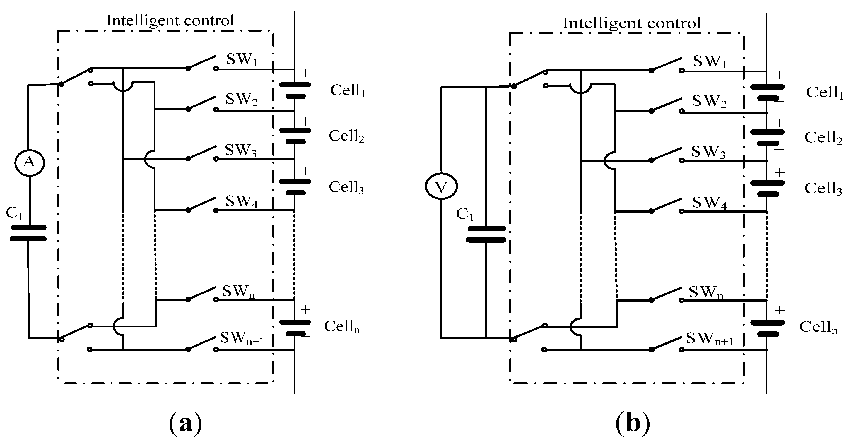
2.2. Single Switched Capacitor (SSC) Topology

Shuttling-capacitor-cell-balancing-topologies shuttle the energy between cells with capacitor. There are four kinds of configurations commonly used in this method [29,30]: basic switched capacitor (SC), double-tiered switched capacitor (DTSC), single switched capacitor (SSC), and modularized switched capacitor (MSC). For the former two topologies (SC/DTSC), intelligent control strategies are not needed. Both of them can work in charging or discharging modes. The equalization time of them is relatively longer than the latter two. For the modularized switched capacitor (MSC), the battery pack was divided into several groups or modules. There is an equalization system operating on module level, and in each module, there is a separate equalization system to deal with the individual cells. For the SSC topology, it needs only one capacitor and n + 5 bi-directional switches to balance n individual cells. Many advanced balancing strategies can be used for increasing the balancing speed and effectiveness. When the number of cells in a pack is greater than five, it is a very cost-efficient topology. In the proposed algorithm, we check our data stream mining based balancing strategy on this topology. This can be seen in Figure 1a in which an ampere-meter was connected to the capacitor to measure the shuttling capacities between cells. However, in practice use, the current sensors are more noise sensitive than voltage sensors. So, as an alternative, topology (a) can also be replaced by topology (b) where the shuttling information can be obtained by adding a voltage sensor in parallel with the capacitor. The shuttling capacity can be periodically calculated by Equation (12). In fact, the data-stream-mining based balancing strategy can be used in many other topologies. We select the SSC topology just for illustrating the usage of it.

Figure 1. Single switched capacitor topology with (a) current sensor and (b) voltage sensor.

Figure 1. Single switched capacitor topology with (a) current sensor and (b) voltage sensor.

3. Data-Stream-Mining Based Battery Equalization Method

3.1. Extracting Summary Information

In this section, we present our deterministic algorithm to estimate the shuttling capacities for cells. With the given topology (SSC), duty cycle was used to control the switched capacitor. The cycle period T is fixed, the idealized capacitor charges during the half cycle D1 and discharges during the other half cycle D2. The instantaneous current of capacitor C₁ and the charge/discharge cells were recorded simultaneously.

Definition 1. (Shuttling electric charge quantity of cell_n, Q_n(t)). Let i(t) be the instantaneous current shuttling between cell_n and capacitor C₁ (the symbol of it is positive when the instantaneous current flows from cell_n to capacitor C₁; Otherwise, is negative), Q_n⁰ be initial Shuttling electric charge quantity of cell_n. The shuttling electric charge quantity of cell_n, Q_n(t), can be expressed like this,

$$Qn(t)={\displaystyle {\int }_0^{t}i(t)dt+Q_n^0}$$

(1)

Definition 2. (Window, window_j). Let the records of measured current i_c of capacitor C₁ and the identifier of charge/discharge cell be a data stream, the incoming stream is conceptually divided into windows. Each window is a completed charging or discharging process, the width of which was decided by the end-of-charging voltage threshold and end-of-discharging voltage threshold. We label the windows with window_j, the value of it is the number of charging and discharging processes.

Definition 3. (Data structure, DS). DS is a set of entries of the form (n, Q_n), where n is an identifier of cell_n, Q_n is an estimated shuttling electriccharge quantity of cell_n.

Algorithm

(1) Initializing DS. Clean the records in it.

(2) Recording data. Every times the current sensor inputs a new record for celln, we first lookup DS to see whether or not an entry for it has exist. If finds, update the entry by incrementing the shuttling electric charge quantity of celln, Qn(t). Otherwise, creates a new entry (n, Qn) for it.

(3) Does a window boundary arrives? Yes, go (4); No, go (2).

(4) Moving the DS to a special memory DS* (DS* was used for directing the balancing processes in the proposed control strategy, we can see this in Section 3.2); go (1).

Examples 

To clearly show the extracting process of summary information, we give a sketch to show the whole changing process of the balanced capacities and the capacitor current. The micro-changes of integral current in 40–70 s were amplified in Figure 2a the whole summary in formation is shown in Figure 2b. For the Capacitor, the balanced current in half cycle D1 were expressed by a₁, a₂, …, a_n. The corresponding current of cell₁–cell_n in half cycle D1 were A₁, A₂, …, A_n. In half cycle D2, the balanced current were expressed by b₁, b₂, …, b_n, the corresponding current of cell₁–cell_n were B₁, B₂, …, B_n.

Figure 2. (a) A section of the summary information (40–70 s); (b) The summary information.

Figure 2. (a) A section of the summary information (40–70 s); (b) The summary information.

3.2. The Proposed Balancing Strategy

In this paper, the summary information was stored in a memory, the power of which was supplied by an independent battery. So, it remains available for every charging or discharging cycle. The cycle period T of duty cycle is fixed, which contains one half cycle D1 (releasing charge to the capacitor) and one half cycle D2 (getting charge from the capacitor). The balancing strategy directly impacts the convergence speed and the balance effectiveness. Considering the achievement of simple architecture and good performance, the proposed algorithm and its flowchart were designed like this:

(1)

Data acquiring: Reads in the summary information from DS*, ranks the entry (n, Q_n) with the values of Q_n.

(2)

Voltage monitoring: Check the terminal voltages of cells. If the terminate voltage, V_n, of a cell, cell_n, reaches the end-of-charge/end-of-discharge voltage threshold, V_high/V_low, closes the charge/discharge process. Begins a new window and go to (1). Otherwise, go to (3).

(3)

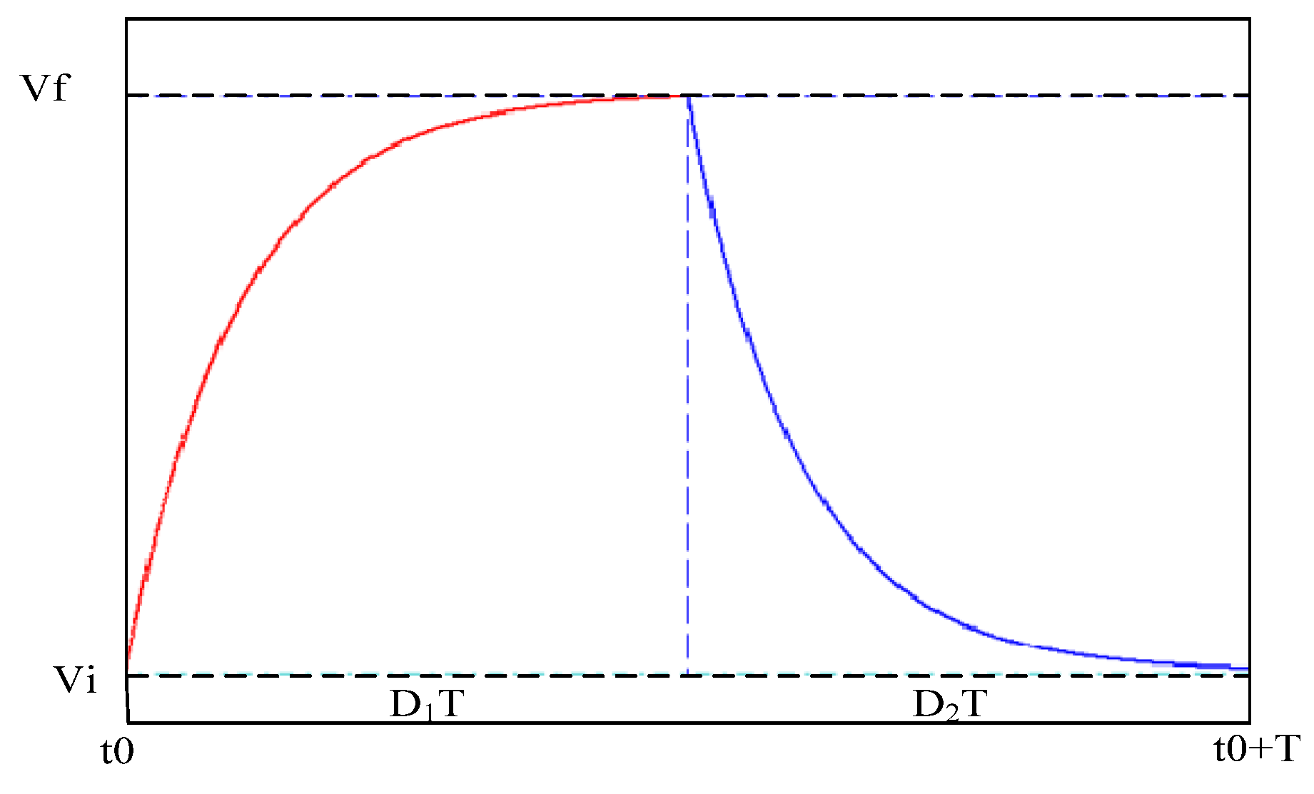
Period D1: Searches an entry (n, Q_n) in DS*, the value Q_n of which is the largest one; closes the two neighboring switchers of cell_n and shuttles the charges from cell_n to capacitor C₁; updates the shuttling electric charge quantity, Q_n (Q_n = Q_n − Q′). Q′ is the shuttled electric charge quantity in period D1.

(4)

Period D2: Searches an entry (m, Q_m) in DS*, the value Q_m of which is the lowest one; closes the two neighboring switchers of cell_m and shuttles the charges from capacitor C₁ to cell_m; updates the shuttling electric quantity, Q_m (Q_m = Q_m + Q″). Q″ is the shuttled electric quantity in period D2.

(5)

Shutting electric charge quantity checking: If all of the Q_i in DS* meet the conditions of “|Q_i| ≤ Δ”, go to (6). Otherwise, go to (2) (Δ is a capacity-updating parameter).

(6)

Balancing the cells with a traditional voltage-based strategy.

(7)

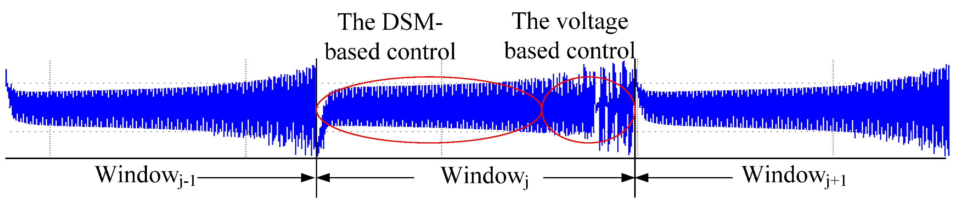
Checking the window boundaries: Does a window boundary arrive? Yes, delete the entries (n, Q_n) in DS*, reads in new entries from DS and go to (1). No, go to (6).

In the procedure, steps (1)–(5) were directed by DSM-based strategy. Step (6) was directed by voltage-based strategy.

3.3. Strategy Analysis

For the SSC balancing topology, the efficiency of energy shuttling strategy is a function of the voltage difference (V_diff), switching frequency (F), capacitor value (C), series equivalent resistor (R_s) and other parameters. Since the purpose of this manuscript is to present a DSM based balancing strategy and to show its robustness on voltage noise and inconsistency of cells, we can just compare the proposed strategy with traditional strategies on the same topology and parameters. In fact, when the voltage difference (V_diff) between unbalanced cells is not very large and the capacity difference is very large, the equalization time will increase and the equalization current will be very small. This can be overcome by boosting the capacitor voltage before connecting it to a lower cell [11]. Additionally, super capacitor is a solution for increasing the shuttling efficiency. Traditionally, the balancing strategy of SSC is based on shuttling the energy from higher voltage cell to the lower one.

In the idealized condition, if we assume that the cells have the same resistances and only two kinds of cell voltages were appeared in the system (the high voltage, V_f, and the lower voltage, V_i), the capacitor will be switched from the higher voltage cells (V_f) to the lower ones (V_i). It can be seen in Figure 3. In the duty cycle, T is fixed, and D1 and D2 are set to 50%; we can describe the shuttling process like this:

Figure 3. The voltage changes of the capacitor C₁.

Figure 3. The voltage changes of the capacitor C₁.

Let R_n be the resistance of cell_n, R_c be the resistance of capacitor C₁. In a charging process, if the capacitor C₁ was connected to cell_n whose voltage is greater than the initial voltage of the capacitor, V_i, the corresponding capacitor voltage V_{c_charging} and current i_{c_charging} can be formulated with Equation (2) [19,31].

$$\tau =(R_n+R_c)C$$

$$V_{c\_ch\arg ing}=(V_f-V_i)(1-e^{-\frac{t-t_0}{\tau }})+V_i=V_{diff}(1-e^{-\frac{t-t_0}{\tau }})+V_i$$

$$i_{c\_ch\arg ing}=C\frac{d{V}_c}{dt}=C\frac{1}{\tau }{V}_{diff}{e}^{-\frac{t-t_0}{\tau }}=\frac{V_{diff}}{R_n+R_c}{e}^{-\frac{t-t_0}{\tau }}$$

(2)

Let i_{c_charging} be the instantaneous current flowing from cell_n to the capacitor C₁, Q_n⁰ be initial Shuttling electric quantity of cell_n.

$$Qn(t)={\displaystyle {\int }_{t0}^t{i}_{c\_ch\arg ing}dt+Q_n^{t_0}}$$

$$Qn(t-t_0)={\displaystyle {\int }_{t0}^t{i}_{c\_ch\arg ing}dt}={\displaystyle {\int }_{t0}^t\frac{V_{diff}}{R_n+R_c}\cdot e^{-\frac{t-t_0}{\tau }}dt}$$

According to the definition of Shuttling electric charge quantity, the shuttling electric charge quantity of cell_n in a D₁T circle, Q_n(t_D1), can be expressed by,

$$Qn(t_{D1})={\displaystyle {\int }_0^{D_{1}T}{i}_{c\_ch\arg ing}dt}=\frac{V_{diff}}{R_n+R_c}{[-\tau \cdot e^{-\frac{t-t_0}{\tau }}]}_0^{D_{1}T}=C\cdot V_{diff}[-e^{-\frac{D_{1}T}{\tau }}-1]$$

Similarly, in D₂T circle, if the capacitor C₁ was connected to Cell_m whose voltage is less than the initial voltage V_f of the capacitor, the corresponding capacitor voltage V_{c_charging} can be formulated with Equation (3). The shuttling electric charge quantity of cell_m, Q_m(t_D2), can be expressed by Equation (4).

$$V_{c\_ch\arg ing}=(V_f-V_i)(1-e^{-\frac{t-t_0}{\tau }})+V_i=V_{diff}(1-e^{-\frac{t-t_0}{\tau }})+V_i$$

(3)

$$Qm(t_{D2})={\displaystyle {\int }_0^{D_{2}T}{i}_{c\_disch\arg ing}dt}=\frac{V_{diff}}{R_m+R_c}{[-\tau \cdot e^{-\frac{t-t_0}{\tau }}]}_0^{D_{2}T}=C\cdot V_{diff}[-e^{-\frac{D_{2}T}{\tau }}-1]$$

(4)

From Equations (2) and (4) we can see that the shuttling electric charge quantity for a cell is proportionate to the voltage difference.

For a battery pack consisted of N individual cells in series (Cell_i, i $\in$ [1, N]), each of them has a different rated capacity and was initialized with their rated capacity C_i. Without current loss and balancing strategy, the SOC of the Cell_i can be expressed by this,

$$SO{C}_{i,t}=\frac{C_i-{\displaystyle {\int }_0^{t}Id\tau }}{C_i}$$

(1)

For lithium-based batteries, the OCV-SOC characteristic curves (charge/discharge) in the area of 10%–90% is a flat and linear one. So, we can approximately express the OCV like this,

$$OC{V}_{i,t}=OC{V}_{i,0}+k_i\times SO{C}_{i,t}=OC{V}_{i,0}+k_i-k_i\cdot \frac{{\displaystyle {\int }_0^{t}Id\tau }}{C_i}$$

For two individual cells (cell_j and cell_k), if the rated capacities of cell_j, C_j, is greater than that of cell_k, C_k, and the parameter k_i has the same value as k_k, then, the difference of OCV_j,t and OCV_k,t can be expressed like this,

$$OC{V}_{j,t}-OC{V}_{k,t}=k\cdot [\frac{{\displaystyle {\int }_0^{t}Id\tau }}{C_k}-\frac{{\displaystyle {\int }_0^{t}Id\tau }}{C_j}]=k\cdot [\frac{1}{C_k}-\frac{1}{C_j}]\cdot {\displaystyle {\int }_0^{t}Id\tau }$$

(5)

In Equation (5), the values of k, C_j and C_k are fixed. So, when no balancing strategy was used, the voltage difference between cells will enlarge with the increasing of charge/discharge time, correspondingly.

When voltage based balancing strategy was used and only two cells, cell_j and cell_k, were used in a pack, Equation (5) can be expressed like this,

$$OC{V}_{j,t}-OC{V}_{k,t}=k\cdot [\frac{{\displaystyle {\int }_0^t(I_0-I\prime )d\tau }}{C_k}-\frac{{\displaystyle {\int }_0^t(I_0+I\prime )d\tau }}{C_j}]=k\cdot [\frac{1}{C_k}-\frac{1}{C_j}]\cdot {\displaystyle {\int }_0^t{I}_{0}d\tau }-k[\frac{1}{C_k}+\frac{1}{C_j}]\cdot {\displaystyle {\int }_0^{t}I\prime d\tau }$$

(6)

where I₀ is the charge/discharge current and I′ is the shuttling current. The difference of OCV_j,t and OCV_k,t is decided by the parameters of t, k, C_k, C_j, I₀ and I′.

(2)

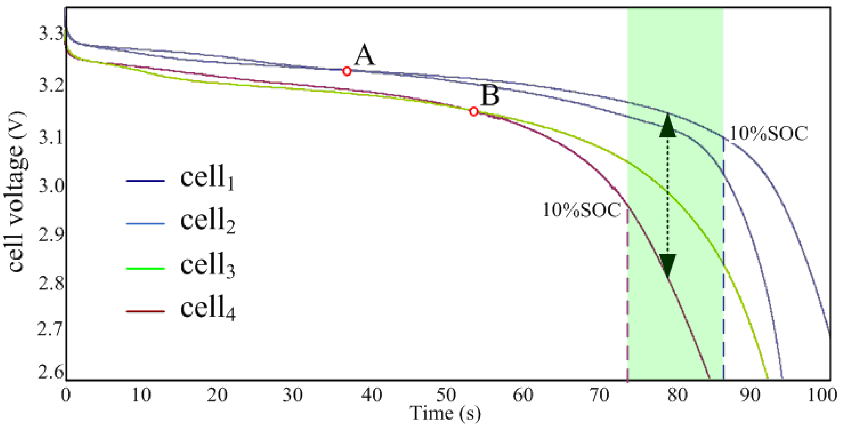
However, for two different cells, cell_j and cell_k, if at time t, one OCV-SOC characteristic curve of them keeps in the area of 10%–90% and the other OCV-SOC characteristic curve goes into the area of 0%–10%, then, with the increase of time t, the voltage difference between them will enlarge quickly. It can be seen in Figure 2, where in the green area, the voltage difference between cell₄ and cell₁ is very large. In this condition, the shuttling efficiency of the current increases with time. With the same probability distribution of the noises, the larger the voltage difference between cells become, the less the probability for mistakenly selecting the cells to shuttle current will be.

So, in the proposed balancing strategy, two kinds of control models were used in sequence. The first one is DSM-based control strategy (in Steps 3–5), in which the shuttling cells and the transfer sequence were decided by summary information obtained. The second one is voltage-based control balancing strategy (in Step 6). If the DSM-based control strategy has finished and the window boundary did not arrive, the balanced cells and the transfer sequence were decided by the cell voltage difference. This can be seen in Figure 4, where two different control strategies appeared in the same window, window_j. In the first step, the DSM-based control strategy was used. The cells were dynamically selected to release/absorb charges by their summary information obtained in the previous window, window_j−1. Once the summary information is exhausted (|Q_i| ≤ Δ), the second step (voltage-based control) will begin until the window boundary arrives.

Figure 4. The summary information and its changing process.

Figure 4. The summary information and its changing process.

3.4. Validity Analysis

To roughly estimate the efficiency of the two strategies, we give some assumptions below:

(1)

Each adjacent window, Window_j−1 and Window_j, has the same number of D1/D2 periods (ND₁ = ND₂).

(2)

In every half cycle, D1, if we properly select cells to shuttle current, all of the shuttling currents of them have the same value Q_T′. If we wrongly select cells to shuttle current, all of the shuttling currents of them have the same value Q_F′.

(3)

In every half cycle, D2, if we properly select cells to shuttle current, all of the shuttling currents of them have the same value Q_T*. If we wrongly select cells to shuttle current, all of the shuttling currents of them have the same value Q_F*.

(4)

In each window, the probability of rightly selecting cell_i in D1 is p_(i,T) and the probability of wrongly selecting Cell_i in D1 is p_(i,F).

(5)

In each window, the probability of rightly selecting cell_m in D2 is p_(m,T) and the probability of wrongly selecting Cell_m in D1 is p_(m,F).

In fact, in period D1/D2, if we properly select Cell_i to shuttle current, the absolute value of the shuttling currents |Q_i′| will be a large value. If we mistakenly select Cell_j to shuttle current, the absolute value of the shuttling currents |Q_j′| will be a small value. Thus, in the same window, window_j−1, the total shuttling currents Q_i of cell_i in half cycle D1 can be calculated by

Q_i = Q_T′ × ND₁ × p_(i,T) + Q_F′ × ND₁ × p_(i,F)

(7)

When

Q_T′ >> Q_F′, Q_i ≈ Q_T′ × ND₁ × p_(i,T)

(8)

For two individual cells, Cell_j and Cell_i, if Q >> Q_i, we can get p_(j,T) >> p_(i,T).

In step (3) of the proposed strategy, the more the value of Q_j is, the earlier the cell_j will be selected to release current. So, in the former K times balancing, the right cells will be selected to release charges with a larger probability than the later ND-K times.

For M individual cells, the shuttling currents of them in half cycle D1 can be expressed by Equation (8). With the conditions of “|Q_n| ≤ Δ”, we can get

Q_n ≈ Q_T′ × ND₁ × p_(n,T) > Δ

thus

p_(n,T) > Δ/(Q_T′ × ND₁)

(9)

So, by setting a proper parameter Δ, we can select K proper cells with a large probability p, p ≥ Δ/(Q_T′ × ND₁).

The similar results can also be obtained in half cycle D2, in which the shuttling currents of the cells were negative. In window, window_j−1, the total shuttling currents Q_m of Cell_m in half cycle D2 can be calculated by

Q_m = Q_T* × ND₂ × p_(m,T) + Q_F* × ND₂ × p_(m,F)

(10)

when

Q_T* << Q_F*, Q_m ≈ Q_T* × ND₂ × p_(m,T)

(11)

For two individual cells, Cell_j and Cell_m, if Q_j << Q_m, we can get p_(j,T) >> p_(m,T).

With the conditions of “|Q_n| ≤ Δ”, we can get

|Q_n| ≈ |Q_T*| × ND₂ × p_(n,T) > Δ

thus

p_(n,T) > Δ/(|Q_T*| × ND₂)

(12)

By setting a proper parameter Δ, we can also select K* proper cells with a large probability p, p ≥ Δ/ (Q_T* × ND₂).

4. Simulations

MATLAB/Simulink is a frequently-used software for modeling and simulating dynamic systems. In this section, we simulate the SSC balancing topology with it. Five lithium-ion batteries with different capacities were used for the simulation and comparison. The nominal voltage, rated capacity, initial SoC, maximum capacity, fully charged voltage, internal resistance were, respectively, “3.2 V, 4 Ah, 100%, 4 Ah, 3.72 V, 0.008 Ohms”, “3.2 V, 3.8 Ah, 100%, 3.8 Ah, 3.72 V, 0.0084 Ohms”, “3.2 V, 3.6 Ah, 100%, 3.6 Ah, 3.72 V, 0.0088 Ohms”, “3.2 V, 3.4 Ah, 100%, 3.4 Ah, 3.72 V, 0.0094 Ohms” and “3.2 V, 2.5 Ah, 100%, 2.5 Ah, 3.72 V, 0.0128 Ohms”. MOSFET switches were used in the simulation, the internal resistance R_on, snubber resistance R_s, Snubber capacitance were, respectively, 0.001 Ohms, 100,000 Ohms and 250 nF. The capacitor used in this simulation has a capacity of 10 F, the initial voltage of it was set to 2.5 V. The period T of the duty cycle is fixed to 2 s, D1 and D2 were both set to 1 s.

4.1. The Influences of Noise

To clearly show the noise influences on cells’ shuttling currents and voltages in Figure 5, we compared shuttling currents of Cell₁–Cell₅ and Capacitor C₁. It can be seen that, when no noise was overlaid on the measured terminate voltages, the “high voltage cell-capacitor-low voltage cell” shuttling strategy is effective. The cells (Cell₁ and Cell₂) with high rated capacity (4 Ah, 3.8 Ah) release charges regularly and the cell (Cell₅) with lowest rate capacity (2.5 Ah) absorbs charges regularly too. At the same time, with the increasing of the discharge time, the difference of the terminate voltages between the cell (with high rated capacity) and the cell (with low rate capacity) enlarges, so as to the increasing shuttling currents (in other conditions, whether or not the difference of cell voltages increases is determined by parameters t, k, C_k, C_j, I₀ and I′, together; this can be seen in Equation (6)). On the contrary, when a random noise [−0.2 V–0.2 V] was overlaid on the measured terminate voltages, the balancing result of the traditional shuttling strategy did not perform very well. Some inappropriate cells were selected to release or absorb charges. This leads to invalid charge shuttling. It can be clearly seen in Figure 5b and Figure 6b, the shuttling currents and the voltage-changes of Cell₁–Cell₅ were very irregular. In the condition of no-noise, there is no shuttling currents between C₁ and Cell₃ or Cell₄. However, when the random noises were overlaid on the measured terminated voltages, the shuttling currents between C₁ and Cell₃ or Cell₄ appeared.

Figure 5. The shuttling currents of Cell₁–Cell₅ and Capacitor in conditions of (a) no-noise and (b) noise.

Figure 5. The shuttling currents of Cell₁–Cell₅ and Capacitor in conditions of (a) no-noise and (b) noise.

Figure 6. The voltages of Cell₁–Cell₅ and Capacitor₁ in conditions of (a) no-noise and (b) noise.

Figure 6. The voltages of Cell₁–Cell₅ and Capacitor₁ in conditions of (a) no-noise and (b) noise.

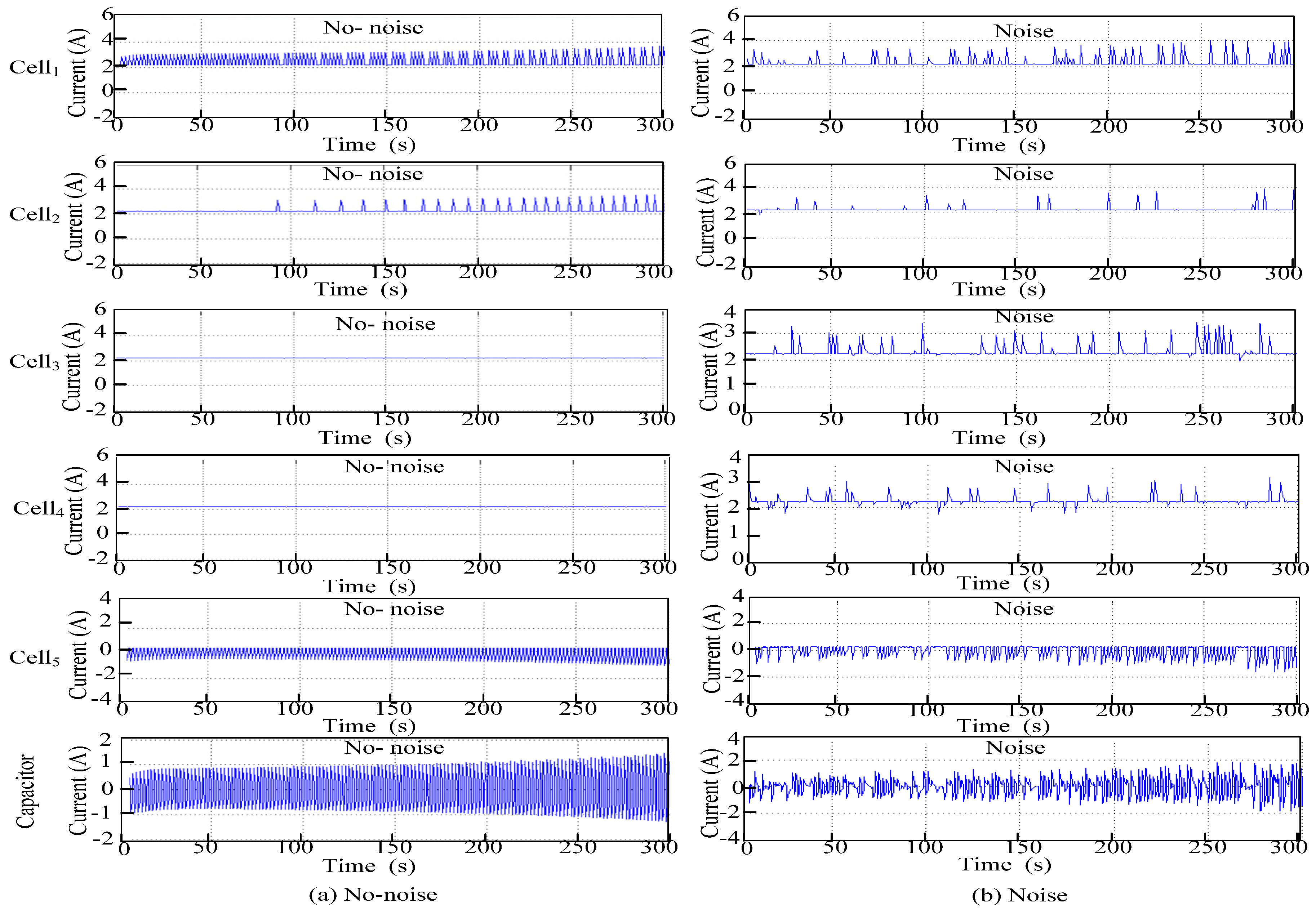
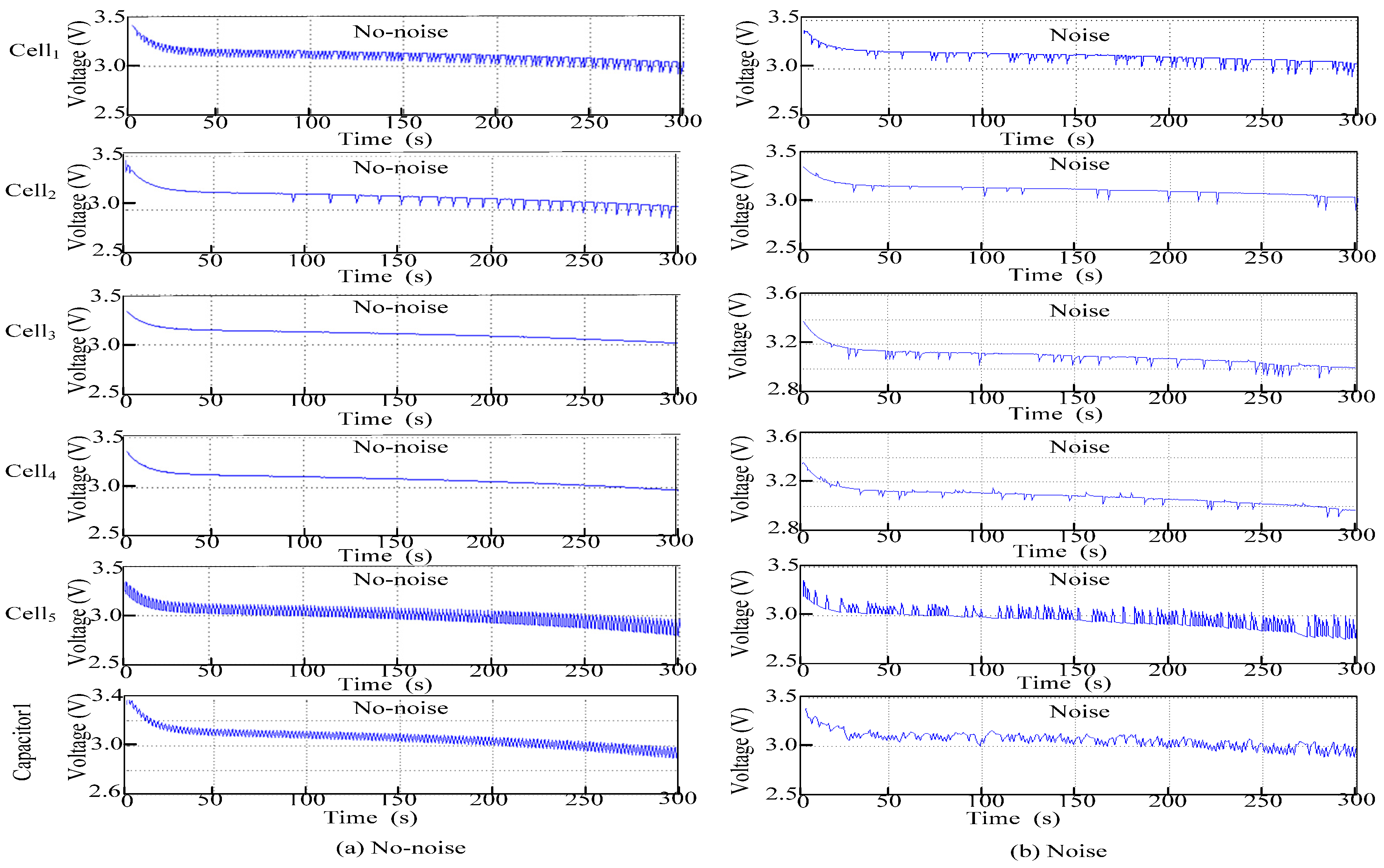
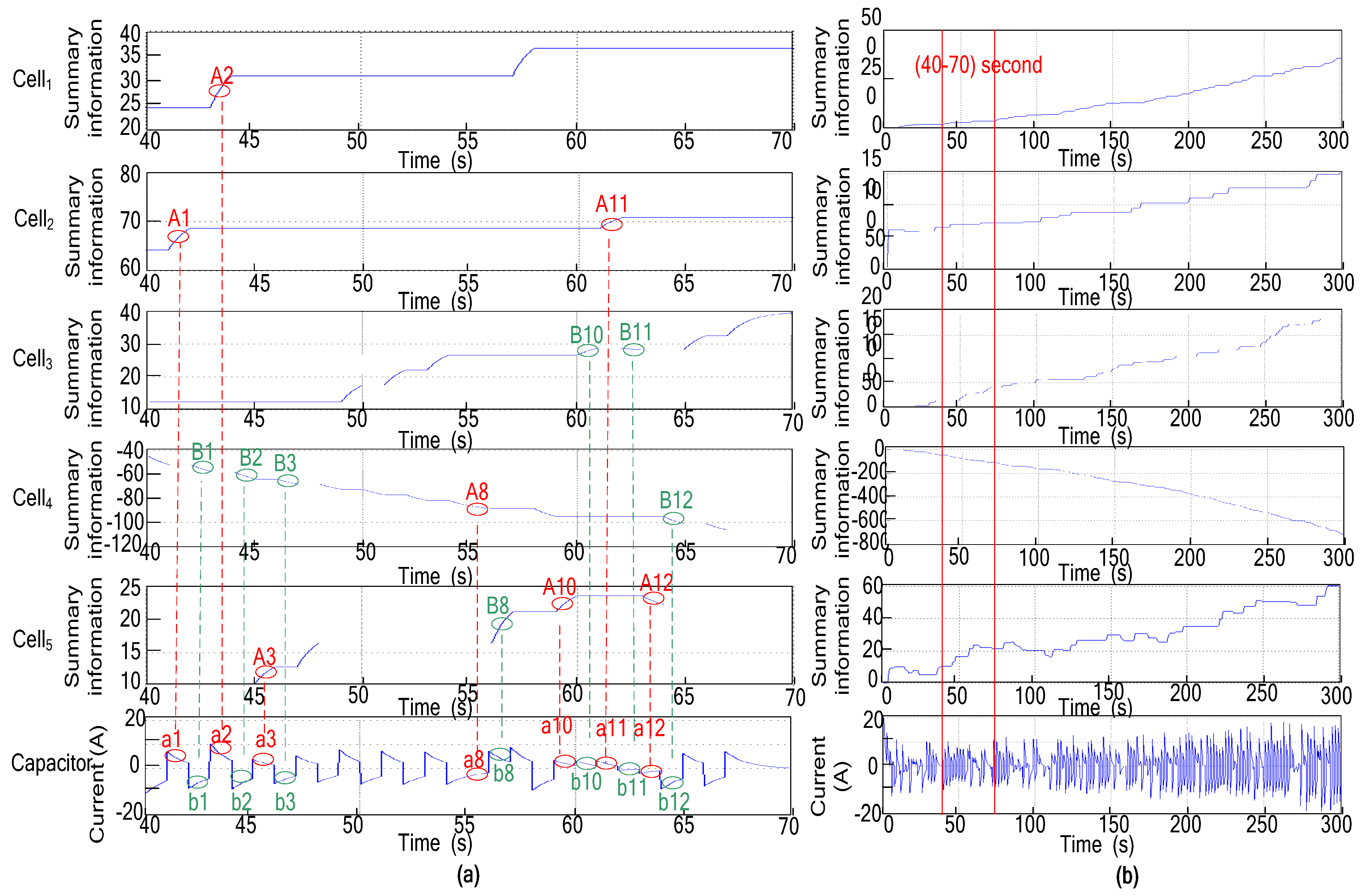
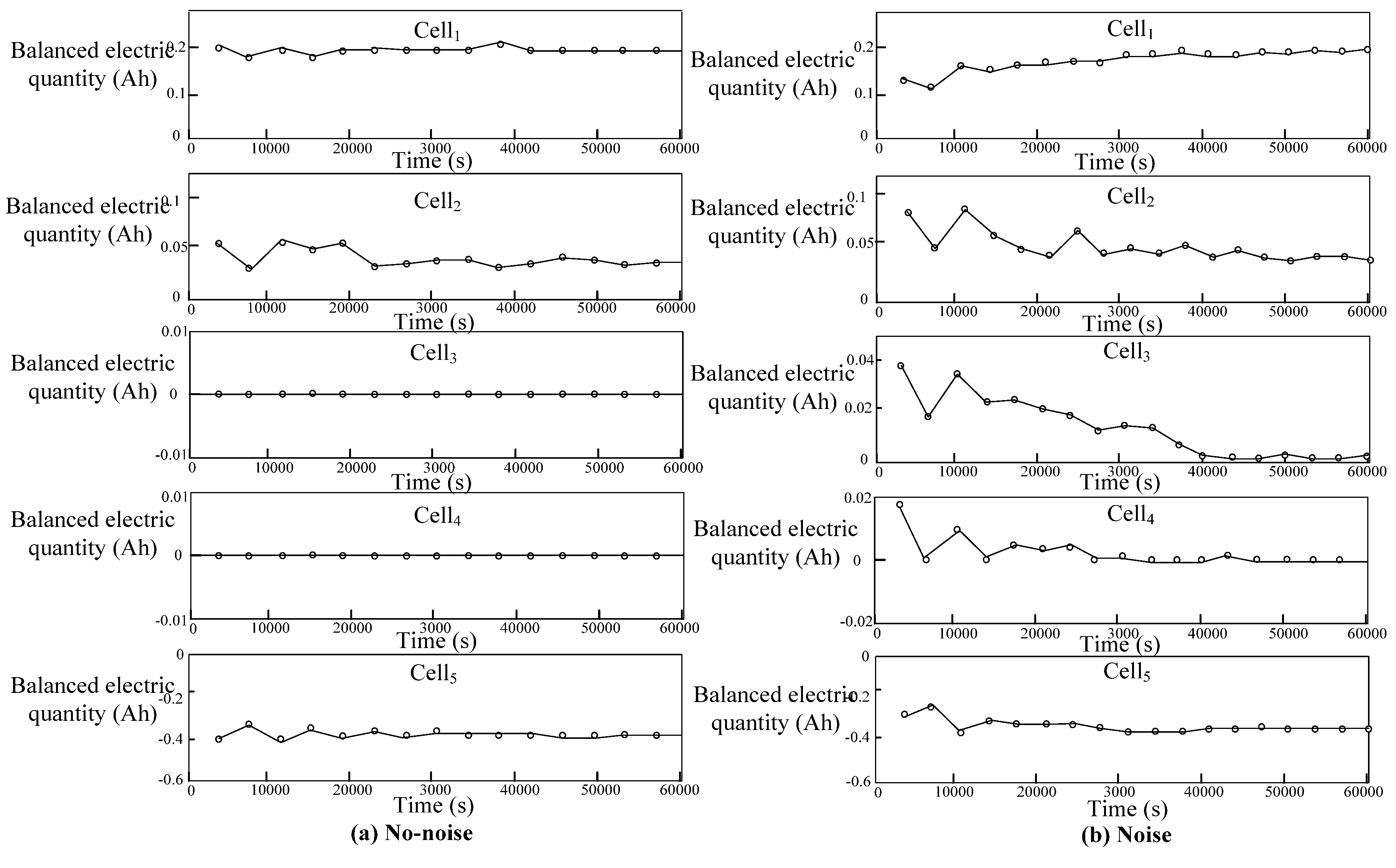
4.2. Extracting the Summary Information in Noise or No-Noise Conditions

In this section, we extract the summary information on the shuttling capacities and record it in each charging or discharging cycle. According to Formulas (2) and (4), we can calculate the shuttling capacities for cells in a half duty cycle D1 or D2 like this,

$$Qn(t_{D1})={\displaystyle {\int }_0^{D_{1}T}{i}_{c\_ch\arg ing}dt}=\frac{V_{diff}}{R_n+R_c}{[-\tau \cdot e^{-\frac{t-t_0}{\tau }}]}_0^{D_{1}T}$$

$$Qm(t_{D2})={\displaystyle {\int }_0^{D_{2}T}{i}_{c\_disch\arg ing}dt}=\frac{V_{diff}}{R_m+R_c}{[-\tau \cdot e^{-\frac{t-t_0}{\tau }}]}_0^{D_{2}T}$$

However, the values of the shuttling current used in the above formulas are noise sensitive and difficult to be integrated. Furthermore, the resistances and capacities for cells are very different. To obtain a precise shuttling capacity and simplify the calculating process, we can replace the current sensor with a voltage sensor and fix the period of half cycle D1/D2 with 1 s. This can be seen in Figure 1b. In this way, the shuttling capacity of cell_n, Q_n(Di), in half duty cycle, Di, can be calculated as,

$$Qn(Di)=C(V_{Di}\prime -{V_{Di}}^0)$$

where C, in farads (F), is the capacitance of capacitor C₁. V′_Di and V⁰_Di, are the terminal and initial voltage of the capacitor C₁ in the (Di)th half duty cycle. And then, after the (Di)th half duty cycle, the accumulated shuttling-capacity of cell_n, Q_n(t), can be express like this,

$$Qn(t)=Qn(t-t_0)+Q_n^{t_0}$$

$$={\displaystyle \sum _{Di=1}^{t\backslash (\frac{T}{2})}Qn(Di)+Q_n(t-t\backslash (\frac{T}{2}))}+Q_n^{t_0}$$

$$={\displaystyle \sum _{Di=1}^{t\backslash (\frac{T}{2})}C(V_{Di}\text{'}-{V_{Di}}^0)+Q_n(t-t\backslash (\frac{T}{2}))}+Q_n^{t_0}$$

(13)

In a half-duty cycle Di, if celln was not be selected to shuttle current, then $C(V_{Di}\prime -{V_{Di}}^0)=0$. Otherwise, $C(V_{Di}\prime -{V_{Di}}^0)$ will be accumulated for celln. Thus, if we initialize the shuttling electric quantity of celln, $Q_n^{t_0}$, ignore the minor shuttling electric quantity, Q_n(t − t(T/2)), in a unclosed half-duty cycle, and fix the period of half duty cycle, T/2, (T/2 = 1 s), we can easily calculate the shuttling capacity of cell_n by measuring the voltage of capacitor C₁ every 1 s. In this way, we obtain the current for each cell and record it in each charging or discharging cycle. The shuttling electric charge quantities of cells were shown in Figure 7. We can see that with the data-stream-mining based control strategy, after several charging/discharging cycles (about six discharging cycles and six charging cycles), the summary information for cells in noise or no-noise conditions becomes more and more similar. The reason lies in the self-adjusting ability of the strategy.

Figure 7. The summary information in conditions of (a) no-noise; (b) noise.

Figure 7. The summary information in conditions of (a) no-noise; (b) noise.

In fact, the summary-information-extracting process and the cells-balancing process are two synchronous processes. The newly obtained summary information of window_j in DS, is partly decided by the entries of window_j in DS*, and partly decided by the voltage-based strategy in the last balancing process in window_j. Moreover, it will change into entries in DS* in window_j+1. By periodically discarding a special number of shutting capacity in entries (n, Q_n) in DS* in window_j, (see step 5, “If all of the Q_i in DS* meet the conditions of ‘|Q_i| ≤ Δ’, go to (6); Otherwise, go to (2)”), the most noisy capacity in DS* in window_j was deleted and this part of capacity would be supplemented by the shuttling capacities produced in the voltage-based balancing process within the identical window. In fact, the supplemented capacity is produced at the end of the charge/discharge process. If the capacity difference between cells is very large, the voltage gap of them will be rather obvious in this phase. So, the supplemented capacity is approximately robust to the noise due to the large voltage gap. Thus, with the proposed strategy, the noise in the summary information of DSM-based balancing process can be deleted step by step. In this process, the shuttling capacity in DS* keeps on increasing and the shuttling capacity balanced by the voltage based strategy keeps on decreasing until an equilibrium point appeared, at which the shuttling capacity produced by the voltage based strategy is equal to the capacity-updating parameter Δ.

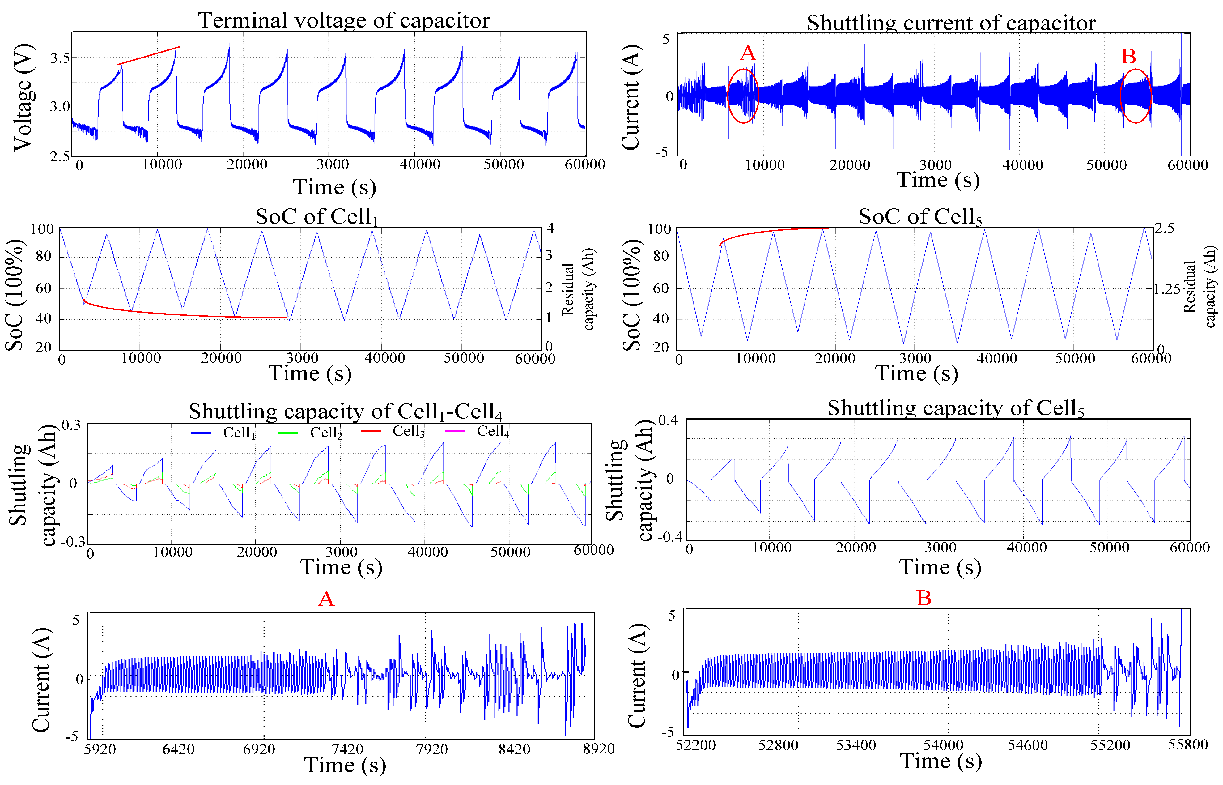
4.3. Working without Terminal Voltage Comparison

In fact, to balance the charges in different N cells, the traditional Terminal Voltage Based Balancing Strategy (TV-BS) needs N-terminal voltage sensors. When lithium-based batteries were used in an electric vehicle, the requirements of high terminal voltage always lead to a large number of cells. This will enlarge the cost of balancing circuits. In this section, we compare our proposed Data Stream Mining Based Balancing Strategy (DSM-BS) in two conditions (with/without terminal voltage comparison). When no terminal voltage comparison was carried out in the DSM-BS, we take only one sensor to periodically check the terminal voltages of cells to ensure that no cell reaches the end-of-charge voltage threshold and the end-of-discharge voltage threshold. In the balancing procedure, strategy steps (1)–(5) keep unchanged. In Step (6), we randomly select cells to absorb or release charges. The purpose of measuring the terminal voltages was not to balance the energies in cells, but to protect them.

From Figure 8, we can find that without terminal voltage comparison, the shuttling currents in the first five charging/discharging circles were very irregular. For example, in area A, the regular discharging process was implemented for 7301 − 5921 = 1380 s. However, in area B (after several circles), the regular discharging process was implemented for 55210 − 52202 = 3008 s. After five charging/discharging cycles, the SOC of Cell₁ arrived its normal value. After four charging/discharging circles, the SOC of Cell₅ arrived its normal value. So, without measuring the terminal voltages of cells, the proposed algorithm can normally work after several charging/discharging circles.

In fact, residual capacity and shuttling capacity are two different concepts. In the most cases, most of the capacities of cells were consumed by the load. Only few capacities were transferred among cells. For example, in Figure 8, the shuttling capacities of cell₁ and cell₅ were approximately converged to 0.2 Ah and 0.3 Ah. In general, the value of the shuttling capacity is decided by several factors. When the capacity differences among cells are very large and the rated power of the load or battery charger is very small, the shuttling capacities of them will be large values. Otherwise, the shuttling capacities will be small.

Figure 8. DSM-based balance (without terminal voltage comparison).

Figure 8. DSM-based balance (without terminal voltage comparison).

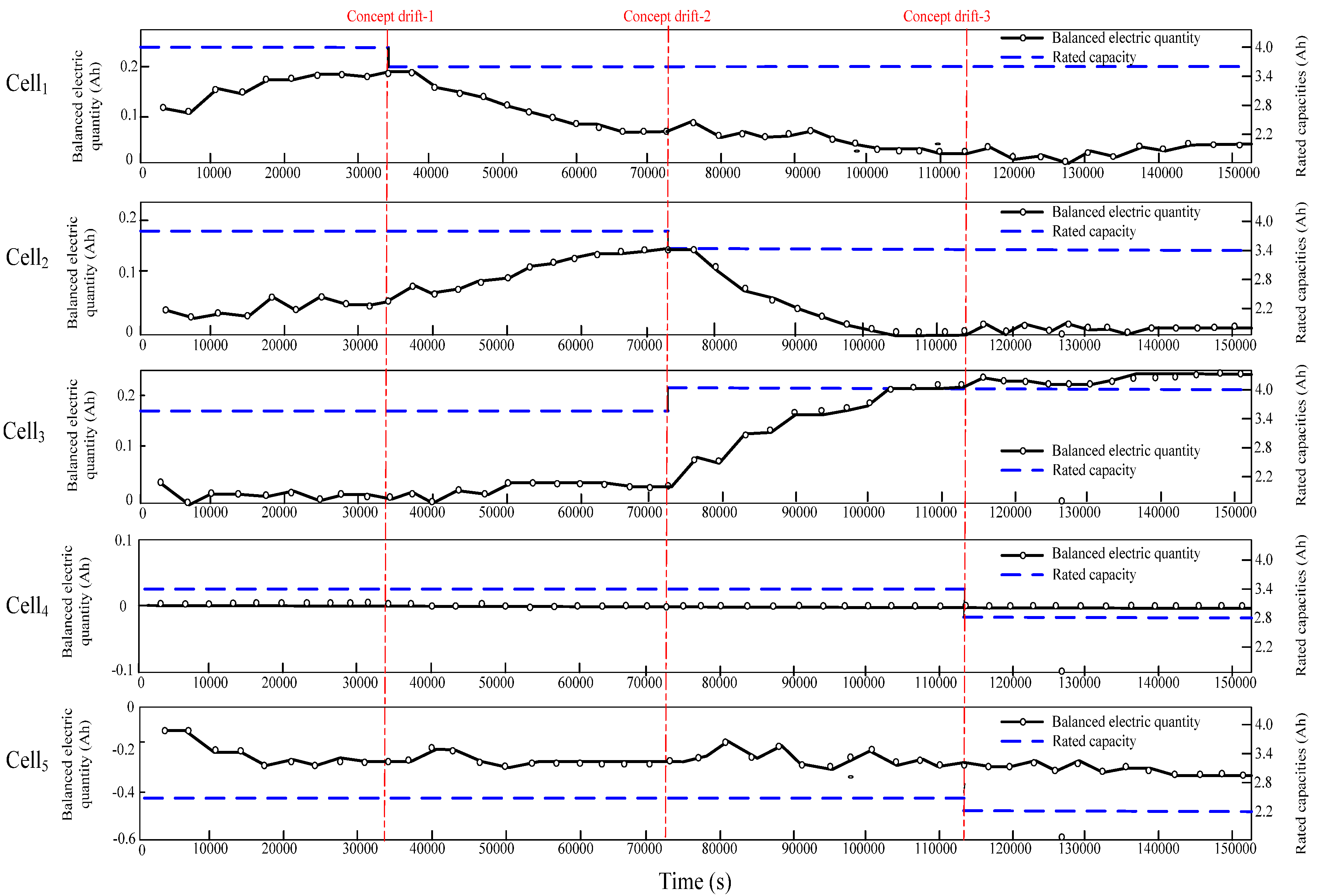
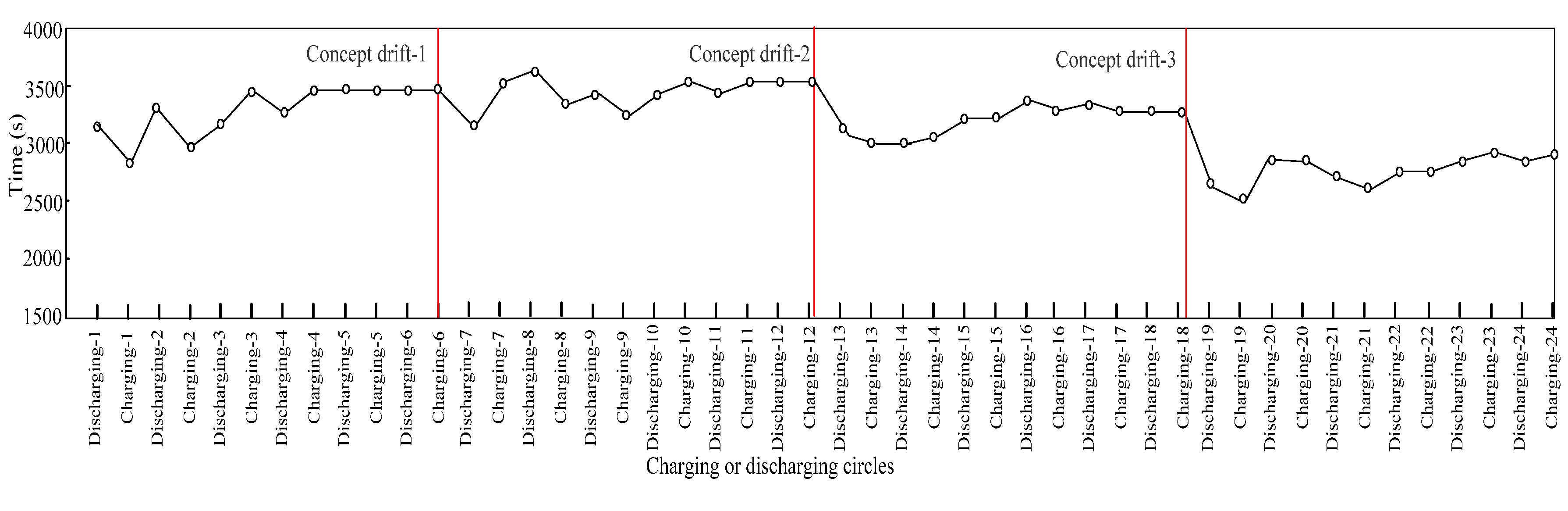
4.4. Dealing with Concept Drifts

In fact, all of the cell capacities in a pack keep decaying in their life cycle. However, the decaying rates of them are so different. It hampers the performance of a given vehicle and leads to many problems. Once the capacity differences between cells were changed, the balancing system must adjust its strategy immediately to reduce its influences on EV. In Figure 9, we extracted the summary information of cells and analyzed the variation trends of them. Totally, three concept drifts (the rated capacity of cell changes with time) were imposed to five cells. In the first concept-drift, the capacity of Cell₁ was set from 4.0 Ah to 3.6 Ah. In the second concept-drift, we changed the capacities of Cell₂ and Cell₃ from 3.8 Ah/3.6 Ah to 3.4 Ah/4.0 Ah. In the third concept-drift, the capacities of Cell₄ and Cell₅ were set from 3.4 Ah/2.5 Ah to 2.8 Ah/2.2 Ah.

The balancing effects of the proposed strategy can be seen in Figure 9 and Figure 10. We can find that, every time a concept drift takes palace, several vibrates of balanced-electric-charge-quantity will appear. After that, the balanced-electric-charge-quantity converged to a fixed value. The time cost for discharging circle and charging circle obeys the similar rules. Whenever a concept-drift takes palace, the charging or discharging circle will be shortened. Then, it slowly increases to a stable cycle. This is because the history information saved in the memory can not be updated at once with the taking place of the concept-drift. So, only sufficient summary information has been accumulated, the proposed strategy can work normally.

Figure 9. The balanced electric charge quantity and rated capacity of cells.

Figure 9. The balanced electric charge quantity and rated capacity of cells.

Figure 10. The balancing time for each discharging/charging circle.

Figure 10. The balancing time for each discharging/charging circle.

5. Experiments

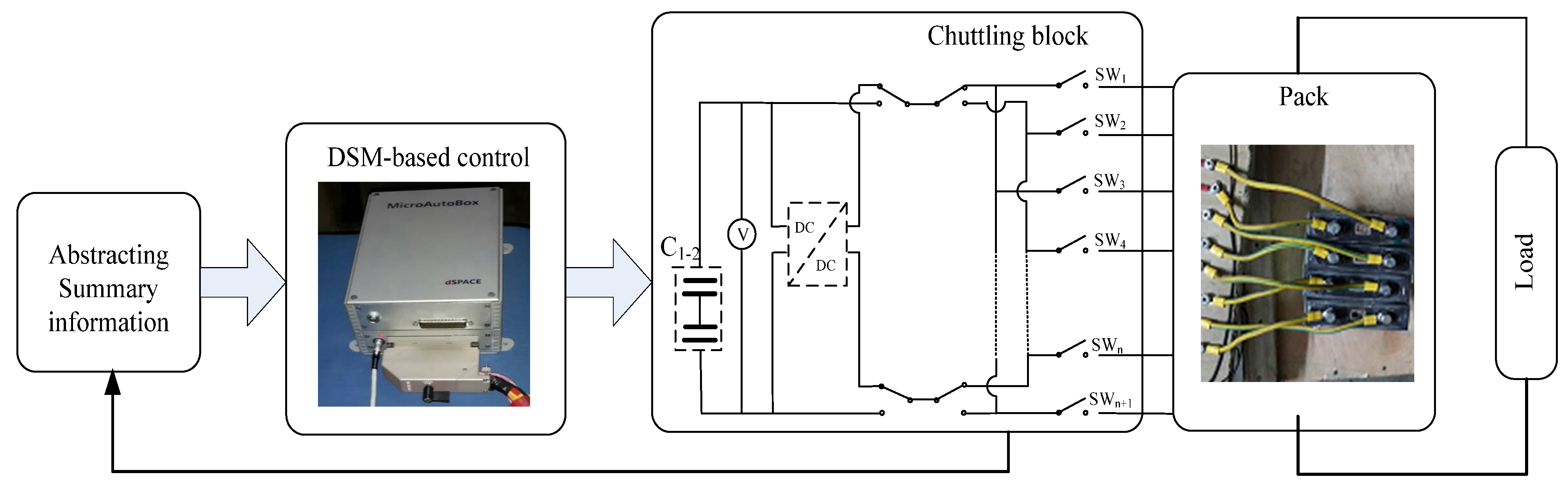
5.1. Experimental Environment

AutoBox is an ideal environment for dSPACE real-time system to implement vehicle control experiments. In this experiment, the two balancing strategies (voltage-based balancing strategy and DSM-based balancing strategy) were carried out in it with the same SSC balancing topology to compare the effectiveness and efficiency. Four old series LFP cells were selected to check the capabilities of discordant cells. All of them have worked for almost three years and came from the same battery pack in an electric vehicle. Their actual capacities were 16.8 Ah, 14.7 Ah, 14.4 Ah, and 12.7 Ah. The full charging voltages of them were set to 3.5 V and the full discharging voltages of them were set to 2.6 V. The maximum continuous discharging current and the maximum charging current were set to 15 A. The circuit consists of five parts: the cells connectors, the switches matrix, two super capacitors (in series), a boosting circuit (DC-DC) and signal acquisition units. The rated voltage of the super capacitor is 2.7 V, the rated input/output voltage of the boosting dc/dc converter is 3/5 V. The measurement and control lines were connected to AutoBox through ADC and DIO ports. We can see the whole BMS architecture in Figure 11.

Figure 11. The global view of control circuit.

Figure 11. The global view of control circuit.

5.2. Discharging Characteristic Curves of the Cells

The discharging characteristic curves of the four cells were shown in Figure 12. From it we can see that the changing processes of voltages were not harmonious. Two obvious cross points “A” and “B” can be seen. “A” is between discharging curves of cell₁ and cell₂, and “B” is between curves of cell₃ and cell₄. If we shuttle the currents between cell₂ and cell₃ (before “A”) or cell₁ and cell₃ (between “A” and “B”) firstly, and then shuttle the currents between cell₁ and cell₄ (after “B”), we cannot obtain a satisfactory balancing result for having select the wrong cells to balance. So, judging the remaining capacity of cells by their terminal voltages will give us the wrong result when there is inconsistency in the cells.

Figure 12. The discharging processes of four cells.

Figure 12. The discharging processes of four cells.

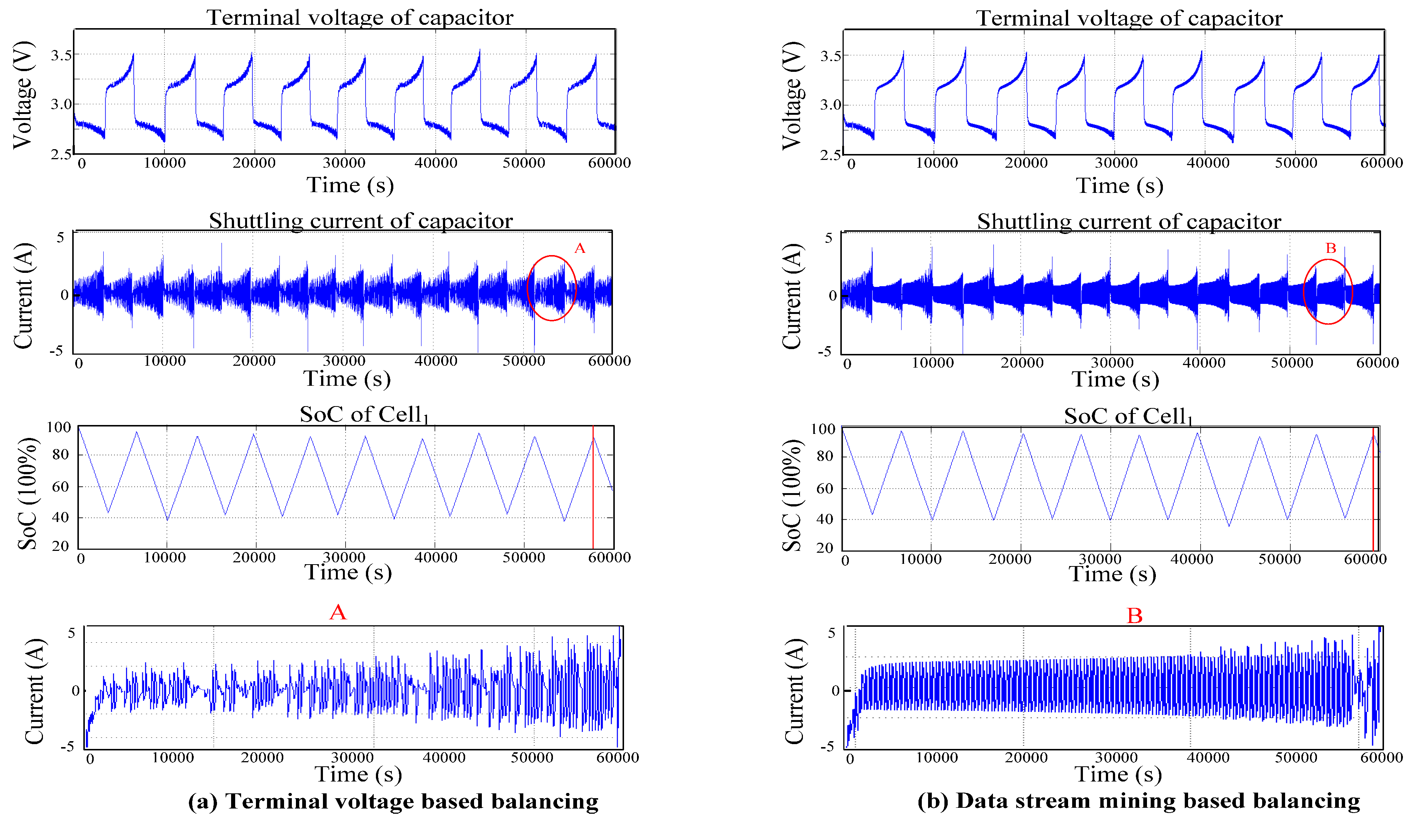
5.3. Strategy Comparison

The corresponding charging/discharging progresses of the two balancing strategies, TV-BS and DSM-BS, are shown in Figure 13. The terminal voltage and shuttling current of capacitor C_1–2, the SOC of cell₁, were also presented. Totally, nine discharging-charging cycles are shown and two of the discharging cycles (A and B) were amplified. It can be seen that, after nine discharging-charging cycles, the traditional balancing algorithm cost 57,500 s, and the proposed balancing algorithm cost 59,500 s. That means DSM-BS strategy is more effective than TV-BS strategy. From the microcosmic views, we can find that when the inconsistencies between cells were very large, the TV-BS strategy cannot select the proper cell to release or absorb charges. This led to the irregular current in Figure 13a. On the contrary, the data stream mining algorithm has the capability of gradually refining the summary information. So, after several charging/discharging cycles, the DSM based balancing strategy can distinguish the cells rightly and shuttle charges with them.

Figure 13. Comparisons of difference balancing strategies: (a) TV-BS and (b) DSM-BS.

Figure 13. Comparisons of difference balancing strategies: (a) TV-BS and (b) DSM-BS.

6. Cost and Computational Time Analysis

For an EV or HEV, the functions of BMS are multifaceted. For example, it measures the cells’ SOC, SOH and temperature; controls the charge/discharge procedure; communicates with other modules; stores historical data; and balances the cells. To efficiently complete these complex functions and manage the great number of cells, many modularized managing systems were proposed [29,30,31,32,33]. In these systems, battery pack is divided into groups of cells. In each of this group, there is an equalization system to balance the subgroup’s cells. Outside the groups, another equalization system is needed to balance the energies between groups. In such a master-slaves control topology, each subgroup balancing circuit is controlled by one slave controller. The group balancing circuit is controlled by another slave controller and the BMS block is managed by the master controller. Generally speaking, the slave microcontrollers need to record the subgroup cells information (voltages, current and temperature) and to make a balancing decision according to the recorded data. The master microcontroller controls the interfacing between the slaves.

In the proposed algorithm, the master-slaves control topology was adopted. The slave circuit comprises five parts: the balancing main circuit (cell connects, switch matrix and super capacitor), the switches driving circuit, power supply circuit, sensors circuit and the microcontroller circuit. The master control circuit consists of a master microcontroller, power supply circuit and several interfacing connect circuits. The main difference between the DSM-BS topology and the TV-BS topology is that, an extra voltage sensor is added to the slave circuit to measure the voltage of the super capacitor. Additionally, extra memory is needed to record the summary information of the balanced capacities. In fact, the efficiency of energy shuttling strategy is a function of the voltage difference (V_diff), switching frequency (F), capacitor value (C), series equivalent resistor (R_s) and other parameters. Due to the introduction of super capacitor, the accessing frequency of voltage sensor C_1–2 and the switching frequency of switcher SW_i in Figure 11 can be reduced to 1 Hz. For a microcontroller, such as PIC18F4550, most of its single-word instructions are executed in a single instruction cycle and the instruction cycle consists of four oscillator periods. If the oscillator frequency is set to 4 MHz, the normal instruction execution time is 1 μs. Thus, the microcontroller has plenty of time to record the cell information and to implement the balancing decision.

7. Conclusions

Cell balancing is an important task for battery management systems. The lifetime and safety of a battery pack is largely decided by the performance of this task. A novel control strategy (data-stream-mining based cell balancing strategy) for SSC balancing system was presented. The comparative study between this approach and the terminal-voltage based cell balancing strategy was performed. The simulation and experimental results has showed that the proposed algorithm has the capability of balancing the individual cells in noise conditions and can deal with the inconsistencies between cells. This is very important for cell balancing systems, the obtained terminal voltages of which are often not harmonious and are interfered with by noise coming from vibration, connection and measurement.

The advantages of the proposed method are:

(1)

The balancing strategy can effectively deal with concept-drifts of cells (the rated capacity changes with time) and automatically adjust the balance process to fit it.

(2)

The proposed algorithm has the capability of balancing the individual cells in noise conditions and can deal with the inconsistencies of cells.

(3)

Data stream mining technique was integrated into the balancing process and the historical information was used to direct the balancing process. The algorithm can not only balance the cell’s residual capacities online, but can also report the their health state indirectly.

References

1. Lu, L.; Han, X.; Li, J. A review on the key issues for lithium-ion battery management in electric vehicles. J. Power Sources 2013, 226, 272–288. [Google Scholar] [CrossRef]
2. Daowd, M.; Omar, N.; van den Bossche, P.; van Mierlo, J. Extended PNGV battery model for electric and hybrid vehicles. J. Int. Rev. Electr. Eng. 2011, 6, 1264–1278. [Google Scholar]
3. Scrosati, B.; Garche, J. Lithium batteries: Status, prospects and future. J. Power Sources 2010, 195, 2419–2430. [Google Scholar] [CrossRef]
4. Lee, Y.-S.; Cheng, M. Intelligent Control Battery Equalization for Series Connected Lithium-Ion Battery Strings. IEEE Trans. Ind. Electron. 2005, 52, 1297–1307. [Google Scholar] [CrossRef]
5. Broussely, M.; Biensasn, P.; Bonhomme, F. Main aging mechanisms in Li ion batteries. J. Power Sources 2005, 146, 90–96. [Google Scholar] [CrossRef]
6. Zheng, Y.; Ouyang, M.; Lu, L.; Li, J.; Han, H.; Xu, L. On-line equalization for lithium-ion battery packs based on charging cell voltages: Part 1. Equalization based on remaining charging capacity estimation. J. Power Sources 2014, 247, 676–686. [Google Scholar] [CrossRef]
7. Zheng, Y.; Lu, L.; Han, X. LiFePO4 battery pack capacity estimation for electric vehicles based on charging cell voltage curve transformation. J. Power Sources 2013, 226, 33–41. [Google Scholar] [CrossRef]
8. Zheng, Y.; Han, X.; Lu, L.; Li, J.; Ouyang, M. Lithium ion battery pack power fade fault identification based on Shannon entropy in electric vehicles. J. Power Sources 2013, 223, 136–146. [Google Scholar] [CrossRef]
9. Hurley, W.G.; Wong, Y.S.; Wölfle, W.H. Self-Equalization of Cell Voltages to Prolong the Life of VRLA Batteries in Standby Applications. IEEE Trans. Ind. Electron. 2009, 56, 2115–2120. [Google Scholar] [CrossRef]
10. Daowd, M.; Omar, N.; van den Bossche, P.; van Mierlo, J. A review of passive and active battery balancing based on MATLAB/Simulink. J. Int. Rev. Electr. Eng. 2011, 6, 2974–2989. [Google Scholar]
11. Manenti, A.; Abba, A.; Merati, A.; Savaresi, S.; Geraci, A. A New BMS Architecture Based on Cell Redundancy. IEEE Trans. Ind. Electron. 2011, 58, 4314–4322. [Google Scholar] [CrossRef]
12. Teofilo, V.L.; Merritt, L.V.; Hollandsworth, R.P. Advanced lithium-ion battery charger. IEEE Aerosp. Electron. Syst. Mag. 1997, 12, 30–36. [Google Scholar] [CrossRef]
13. Lin, C.H.; Wang, C.M.; Chao, H.Y.; Hung, M.H. Dual-balancing control for improving imbalance phenomenon of lithium-ion battery packs. In Proceedings of the IEEE Third International Conference on Sustainable Energy Technologies (ICSET), Kathmandu, Nepal, 24–27 September 2012; pp. 229–234.
14. Lee, Y.S.; Cheng, G.T. Quasi-Resonant Zero-Current-Switching Bidirectional Converter for Battery Equalization Applications. IEEE Trans. Power Electron. 2006, 21, 1213–1224. [Google Scholar] [CrossRef]
15. Moo, C.S.; Hsieh, Y.C.; Tsai, I.S. Charge equalization for series-connected batteries. IEEE Trans. Aerosp. Electron. Syst. 2003, 39, 704–710. [Google Scholar] [CrossRef]
16. Imtiaz, A.M.; Khan, F.H. “Time shared flyback converter” based regenerative cell balancing technique for series connected Li-ion battery strings. IEEE Trans. Power Electron. 2013, 28, 5960–5975. [Google Scholar] [CrossRef]
17. Young, C.M.; Chu, N.Y.; Chen, L.R.; Hsiao, Y.-C.; Li, C.-Z. A single phase multilevel inverter with battery balancing. IEEE Trans. Ind. Electron. 2013, 60, 1972–1978. [Google Scholar] [CrossRef]
18. Maharjan, L.; Inoue, S.; Akagi, H.; Asakura, J. State-of-Charge (SOC)-Balancing Control of a Battery Energy Storage System Based on a Cascade PWM Converter. IEEE Trans. Power Electron. 2009, 24, 1628–1636. [Google Scholar] [CrossRef]
19. Uno, M.; Tanaka, K. Single-Switch Multi-Output Charger Using Voltage Multiplier for Series-Connected Lithium-Ion Battery/Supercapacitor Equalization. IEEE Trans. Ind. Electron. 2013, 60, 3227–3239. [Google Scholar] [CrossRef]
20. Ugle, R.; Li, Y.; Dhingra, A. Equalization integrated online monitoring of health map and worthiness of replacement for battery pack of electric vehicles. J. Power Sources 2013, 223, 293–305. [Google Scholar] [CrossRef]
21. Xu, A.; Xie, S.; Liu, X. Dynamic Voltage Equalization for Series-Connected Ultra-capacitors in EV/HEV Applications. IEEE Trans. Veh. Technol. 2009, 58, 3981–3987. [Google Scholar]
22. Chen, W.-L.; Cheng, S.-R. Optimal charge equalization control for series-connected batteries. IET Gener. Transm. Distrib. 2013, 7, 843–854. [Google Scholar] [CrossRef]
23. Park, H.S.; Kim, C.H.; Park, K.B.; Moon, G.W.; Lee, J.H. Design of a charge equalizer based on battery modularization. IEEE Trans. Veh. Technol. 2009, 58, 3216–3223. [Google Scholar] [CrossRef]
24. Nasraoui, O.; Rojas, C.; Cardona, C. A Framework for Mining Evolving Trends in Web Data Streams using Dynamic Learning and Retrospective Validation. J. Comput. Netw. 2006, 50, 1425–1652. [Google Scholar] [CrossRef]
25. Widmer, G. Tracking Context Changes through Meta-Learning. Mach. Learn. 1997, 27, 256–286. [Google Scholar] [CrossRef]
26. Minku, L.L.; Yao, X. DDD: A New Ensemble Approach for Dealing with Concept Drift. IEEE Trans. Knowl. Data Eng. 2012, 24, 619–633. [Google Scholar] [CrossRef]
27. Minku, L.L.; White, A.P.; Yao, X. The Impact of Diversity on On-Line Ensemble Learning in the Presence of Concept Drift. IEEE Trans. Knowl. Data Eng. 2010, 22, 730–742. [Google Scholar] [CrossRef]
28. Scholz, M.; Klinkenberg, R. Boosting Classifiers for Drifting Concepts. In Intelligent Data Analysis (IDA); IOS Press: Amsterdam, The Netherlands, 2007; Volume 11, pp. 3–28. [Google Scholar]
29. Baughman, A.C.; Ferdowsi, M. Double-tiered switched-capacitor battery charge equalization technique. IEEE Trans. Ind. Electron. 2008, 55, 2277–2285. [Google Scholar] [CrossRef]
30. Kimball, J.W.; Krein, P.T. Analysis and Design of Switched Capacitor Converters. In Proceedings of the Twentieth Annual IEEE Applied Power Electronics Conference and Exposition (APEC’05), Austin, TX, USA, 6–10 March 2005; Volume 1473, pp. 1473–1477.
31. Ben-Yaakov, S.; Evzelman, M. Generic and unified model of Switched Capacitor Converters. In Proceedings of the IEEE Energy Conversion Congress and Exposition (ECCE’09), San Jose, CA, USA, 20–24 September 2009; pp. 3501–3508.
32. Daowd, M.; Antoine, M.; Omar, N.; Lataire, P.; van den Bossche, P.; van Mierlo, J. Battery Management System-Balancing Modularization Based on a Single Switched Capacitor and Bi-Directional DC/DC Converter with the Auxiliary Battery. Energies 2014, 7, 2897–2937. [Google Scholar] [CrossRef]
33. Gallardo-Lozano, J.; Romero-Cadaval, E.; Milanes-Montero, M.I.; Guerrero-Martinez, M.A. Battery equalization active methods. J. Power Sources 2014, 246, 934–949. [Google Scholar] [CrossRef]