Estimating PV Module Performance over Large Geographical Regions: The Role of Irradiance, Air Temperature, Wind Speed and Solar Spectrum

Abstract

We present a study of how photovoltaic (PV) module performance varies on continental scale. Mathematical models have been used to take into account shallow-angle reflectivity, spectral sensitivity, dependence of module efficiency on irradiance and module temperature as well as how the module temperature depends on irradiance, ambient temperature and wind speed. Spectrally resolved irradiance data retrieved from satellite images are combined with temperature and wind speed data from global computational weather forecast data to produce maps of PV performance for Eurasia and Africa. Results show that module reflectivity causes a fairly small drop of 2%–4% in PV performance. Spectral effects may modify the performance by up to ±6%, depending on location and module type. The strongest effect is seen in the dependence on irradiance and module temperature, which may range from −20% to +5% at different locations.

1. Introduction

It is well known that the energy conversion efficiency of photovoltaic (PV) modules depends on a number of different external influences. Among these influences are:

• The reflectivity of the module surface, and in particular the way this reflectivity depends on the angle at which the incoming light hits the module surface [1–3].
• The light conversion efficiency depends on the wavelength of the light. The module efficiency will therefore change with variations in the spectrum of the sunlight [4–11].
• The efficiency depends on the temperature of the PV module [12]. The module temperature will in turn depend on the temperature of the surrounding air, on the light intensity and on the local wind speed [13,14].
• Even when all these influences are held constant, the efficiency will still depend on the light intensity [3,15–17].
• Some PV module types show variations in module efficiency that are caused by long-term exposure to sunlight and/or high temperatures.

All these effects cause the module efficiency to deviate from the efficiency measured under Standard Test Conditions (STC) [18], which defines the rated or nominal power of a given module.

In addition to these effects there are of course, other reasons why the energy production of a given PV system would vary, which range from the details of installation (inclination angle, possible shadows) to the total amount of solar radiation at the site of installation, or the probability of dust or snow deposition. However, these are mostly not intrinsic to the module type and would tend to depend more on the details of installation than on the physical properties of the module. We could say that the effects listed above cause different modules installed in the same way and place to give different power output while these other effects would cause the same module to have different power output when mounted in a different way or place.

This distinction matters because knowledge of the first group of effects will allow potential buyers of PV modules to compare the suitability of different module types even before the details of a PV installation have been chosen.

Studies of the geographical variability of PV performance have been presented by a number of authors, either for a number of discrete locations (an early example is Bücher, 1997 [19]) or over larger geographical regions at regular grid points. These studies have been at the scale of a city [20,21], over parts of a country [22] or at continental scale [3,23]. In some cases, only the variation in solar irradiation is taken into account while other authors include some of the effects listed above.

The availability of solar radiation data from satellite has made it possible to estimate the solar resource at any location over very large geographical areas, typically on a continental scale. Combining these data with temperature and wind data from reanalysis data sets or meteorological models makes it possible to estimate the performance of PV modules taking into account many of the effects that influence their performance, and doing so at any location.

In this study, we will present results of applying models for PV module performance over large geographical areas. The effects considered are shallow-angle reflectivity, spectral sensitivity, as well as the influence of module temperature and irradiance on module power output, including also the cooling effect of wind. The study area comprises Europe, Africa and nearly all of Asia, limited by the availability of solar radiation data from satellite, in this case the European Meteosat satellites. The paper is structured as follows: Section 2 describes the sources of solar radiation and meteorological data. Section 3 presents the mathematical models for PV module performance. Section 4 shows the results of the calculations, including a comparison with calculations for single locations using measured solar radiation and temperature data. Finally, our conclusions are given in Section 5. Please note the table of nomenclature at the end of the paper.

2. Input Data Sets

2.1. Solar Radiation Data

The solar radiation data used in this study are derived from satellite images. All the data have been taken from the European METEOSAT class of geostationary meteorological satellites. These satellites are placed in two different positions, one at 0° longitude (off the coast of West Africa), and one at 57° East longitude, over the Indian Ocean. In practice, the calculation of solar radiation from these satellites’ images is possible over a region that extends 60°–65° away from the satellite’s nadir. Thus, the western satellite covers a region from 65° W to 65° E and from 60° N to 60° S, while the eastern satellite extends from 10° W to 115° E. The western satellite is of the class Meteosat Second Generation. The methods for calculating solar radiation from the data from this satellite are described in [24] (see also [25] for additional validation of the retrieved solar radiation data). The eastern satellite is of the Meteosat First Generation class. The methods used to derive solar radiation have been described in [26] and have been further validated using data obtained when this satellite was situated at 0° as well as its later positions at 63° and 57° [27].

The resulting solar radiation data consist of global horizontal and direct horizontal irradiance, with one value per hour. The spatial resolution used for this study is 3 arc-minutes (about 5 km at nadir).

The algorithms described in [26] can also be used to calculate irradiance in a number of spectral bands. In this case, the data output consists of hourly global and direct horizontal irradiance in 24 spectral bands covering the wavelength range 300–2150 nm.

2.2. Ambient Temperature and Wind Speed Data

There are, to our knowledge, no freely available data sets for ambient temperature and wind speed that cover the whole world at high spatial and temporal resolution. For this study, we have employed the numerical weather forecast data produced by the European Centre for Medium-Range Weather Forecast (ECMWF, www.ecmwf.int). A very large number of physical parameters are available from the numerical weather prediction model. For this study, the parameters used are the north-south direction wind speed component, the east-west direction wind speed component (both at 10 m above ground), and the ambient temperature at 2 m above ground. The temporal resolution is 3 h and the spatial resolution is 7.5 arc-minutes (∼ 14 km). To get the hourly data used in the present study, a linear interpolation is applied. For the wind speed, this entails in the first place, calculating the total wind speed from the two components, and then performing the interpolation.

3. Mathematical Models for PV Performance

3.1. Inclined-Plane Irradiance

The solar radiation data estimated from satellite information consist of the global horizontal irradiance and the direct component also on the horizontal plane. Since most PV installations use inclined (sometimes moving) modules, the irradiance on an inclined plane must be estimated. In this study, the method used is based on the one by [28], see also the validation study by Gracia and Huld [29].

3.2. Angle-of-Incidence (AOI) Effects

When the solar radiation hits the PV module at an angle away from normal to the module’s surface, the reflectivity of the module is generally increased. This reflected radiation does not contribute to the photocurrent, and is assumed here to also not contribute to the heating of the module. (In principle, some of the “missing” light at shallow angle of incidence is not reflected but absorbed in the glass. This effect is ignored here).

In this study, the model used has been taken from the paper of Martin and Ruiz [1]. In this model, the beam and diffuse components are treated separately. The coefficients used are those from [1] that pertain to typical crystalline silicon modules.

3.3. Spectral Effects

The conversion efficiency of PV modules depends on the spectrum of the incoming light. When the module is measured under Standard Test Conditions [18], also the spectrum of the light is specified by the International Standard IEC-60904-3 [30]. If the sunlight spectrum R(λ) is different from the standard at a given location and time, the power output of the module will be different from what would be expected from the value of the total incoming irradiance.

The model to account for this effect has been described in [11] and is very similar to that used by a number of other researchers [8–10]. For a given sunlight spectrum, the effective irradiance G_eff is given by Equation (1):

$$G_{eff}=G\frac{{\displaystyle \int S_r\left(\lambda \right)R\left(\lambda \right)d\lambda }}{{\displaystyle \int S_r\left(\lambda \right)R_{\text{STC}}\left(\lambda \right)d\lambda }}$$

(1)

Here, S_r(λ) is the spectral response of the module under investigation. In Equation (1) the STC spectrum R_STC(λ) is scaled so the broadband irradiance is the same as the broadband irradiance G.

If the spectral effects are taken into account, G_eff replaces G as input in the estimation of the PV module power output.

The spectral response curves of the modules used in this study have been measured at the European Solar Test Installation laboratory of the European Commission Joint Research Centre [31,32].

It should be noted that while an expression like Equation (1) is widely used there also exists more complex models, see for instance [33].

3.4. Module Temperature

The temperature of the module is assumed to be a function of the incident irradiance, the ambient (air) temperature, and the wind speed.

The wind speed data are estimates for a height of 10 m above ground, while most PV installations have the modules located at a lower height above ground. In this study, the formula in Equation (2) has been used to estimate the wind speed at the modules’ height:

$$W_{\mathrm{mod}}={\left(\frac{d_{\mathrm{mod}}}{d_{\text{ane}}}\right)}^{0.2}\cdot W_{\text{ane}}$$

(2)

Here W_mod and W_ane are the wind speed at the module’s height and the wind speed at the anemometer’s height, respectively, and d_mod and d_ane are the height of the modules and the anemometer. For the present study, the module height has been assumed to be 2 m. The wind speed values W_ane are taken from the ECMWF numerical forecast data for wind at 10 m height.

Given the wind speed and the ambient temperature, the module’s temperature is calculated according to the model of Faiman [13] (Equation (3)):

$$T_{\mathrm{mod}}=T_{\text{amb}}+\frac{G}{U_0+U_1{W}_{\mathrm{mod}}}$$

(3)

The two coefficients U₀ and U₁ have been taken from [14], and vary slightly between module types. The values of the coefficients for crystalline silicon and CdTe modules are given in

Table 1. Values of coefficients U₀ and U₁ used in Equation (3) for two types of PV technologies.

Module Type	U0	U1
c-Si	26.9	6.20
CdTe	23.4	5.44

. The CdTe values are taken from

Table 2. Values of coefficients k₁ to k₆ used in Equation (4) for two different PV technologies.

Module Type	c-Si	CdTe
k1	−0.017237	−0.046689
k2	−0.040465	−0.072844
k3	−0.004702	−0.002262
k4	0.000149	0.000276
k5	0.000170	0.000159
k6	0.000005	−0.000006

in [14] while the c-Si values are an average of the results reported in Table 1 in the same paper for the Negev Desert.

It should be noted that the coefficients U₀ and U₁ have been obtained by fitting to measurements made outdoors. In these measurements the temperature of the module was measured by a temperature sensor attached to the back of the module. The estimated temperature T_mod is therefore the temperature at the back of the module, not the true cell temperature.

3.5. PV Performance

The method used in this study can, in principle, use any model for the estimation of PV module performance, provided the output power can be expressed as a function of incident irradiance and module temperature. The model may be in the form of a mathematical expression or it may use discrete measured data and an interpolation method. For the present study we have used the model described in [17]. The validation has shown that the model works well for several different PV technologies. The model was compared to a range of other models in [16] and also found to perform satisfactorily. The model takes the form shown in Equation (4):

$$\begin{array}{l}P\left(G^{\prime },T^{\prime }\right)=G^{\prime }{P}_{\text{STC}}(1+k_1\ln (G^{\prime })+k_2{(\ln (G^{\prime }))}^2+k_3{T}^{\prime }\\ +k_4{T}^{\prime }\ln \left(G^{\prime }\right)+k_5{T}^{\prime }{(\ln (G^{\prime }))}^2+k_6{T^{\prime }}^2)\end{array}$$

(4)

$$G^{\prime }\equiv G/1000W\cdot {\mathrm{m}}^{-2}$$

(5)

$$T^{\prime }\equiv T_{\mathrm{mod}}-25°\mathrm{C}$$

(6)

The coefficients k₁…k₆ must be determined by fitting to measured data. For this study, the coefficients used for c-Si modules are taken from [17], found by combining measured data for 18 c-Si modules and fitting using a least-squares fit. This shows one advantage when using a formula-based model: it is possible to combine data from several PV modules, even if the number of measurements varies between modules, since all the data are used together for the fitting procedure.

For CdTe modules, the corresponding coefficients have been obtained by a least-squares fit to measurements performed at the ESTI (European Solar Test Installation) laboratory [17]. This set of coefficients is somewhat different from that found in [3]. In that study the coefficients were found by fitting to outdoor measurements without correcting for spectral effects.

It should be noted that these coefficients are based on measurements on modules that by now are some years old. Newer CdTe modules may have different properties, especially in regards to their performance at low-light conditions.

The coefficients for c-Si and CdTe are given in Table 2

3.6. Definition of the Module Performance Rati

The models described in the previous subsections give an estimate of the instantaneous output power of PV modules, which will vary strongly with time especially due to changes in the solar irradiance. In order to describe the overall performance of a PV module, we propose the yearly average Module Performance Ratio, MPR_year defined in Equation (7):

$${\text{MPR}}_{\text{year}}=\frac{G_{\text{STC}}\cdot E_{\text{year}}}{P_{\text{STC}}\cdot H_{\text{year}}}$$

(7)

Here G_STC=1000 W · m⁻² is the irradiance at STC conditions, E_year is the total yearly PV energy output at the terminals of the PV module, assuming that the module always works at Maximum Power Point. H_year is the total yearly in-plane irradiation. In a similar way we can calculate MPR taking into account the effect of wind MPR_W,year. Thus, MPR_year is the ratio of the actual energy production to that which would have been obtained if the module had always worked at the conversion efficiency measured at STC.

MPR_year can also be expressed in terms of the annual average energy conversion efficiency of the PV module, ⟨η_year⟩, as the ratio of actual module efficiency to the efficiency under STC conditions, as shown in Equation (8):

$${\text{MPR}}_{\text{year}}=\frac{\langle {\eta }_{\text{year}}\rangle }{{\eta }_{\text{STC}}}$$

(8)

η_STC is the module efficiency under Standard Test Conditions.

The Energy Rating of a module would then consist of a few values of MPR_year for pre-defined climatic zones.

3.7. Calculation over Large Geographical Areas

The methods described in previous subsections have been implemented in a module under the open-source GIS (geographic information system) software GRASS. Calculations are performed for every hour in a given time period. The module inclination angle is assumed constant over the entire region and the modules are oriented so as to face towards the equator.

For each hour, the following parameters are calculated:

• Global inclined irradiance, G
• Global inclined irradiance corrected for AOI effects, G_a
• Spectrally resolved global inclined irradiance, corrected for AOI effects, R_a(λ)
• Module power output for a nominal PV power P_STC = 1 kW_p, taking into account AOI, the effects of temperature and low irradiance, but ignoring the effect of wind (essentially setting U₁ = 0 in Equation (3)
• Module power output P_w, also taking into account wind speed.

The calculation was performed separately for the data of the two satellites. The hourly values were summed to a yearly total irradiation (or PV module energy output), and the two data sets were then merged along the longitude (θ) line θ = 42°30′ E, according to this rule (Equation (9)):

$$D=\{\begin{array}{ll}{D}_w\hfill & \theta <40°\hfill \\ D_e\hfill & \theta >45°\hfill \\ 0.2\left(45°-\theta \right)D_w+0.2\left(\theta -40°\right)D_e\hfill & 40°<\theta <45°\hfill \end{array}$$

(9)

Here D_w and D_e are the values of a given parameter D from the western and eastern satellite, respectively.

Once the total irradiation and the total PV output energy have been calculated, it is possible to calculate the Module Performance Ratio (MPR), as given in Equation (7).

4. Results and Discussion

This section contains the results of the calculation methods described in the previous section in the form of graphs and maps. The data used to produce the figures can be downloaded from the web page containing supplementary data for this paper [34].

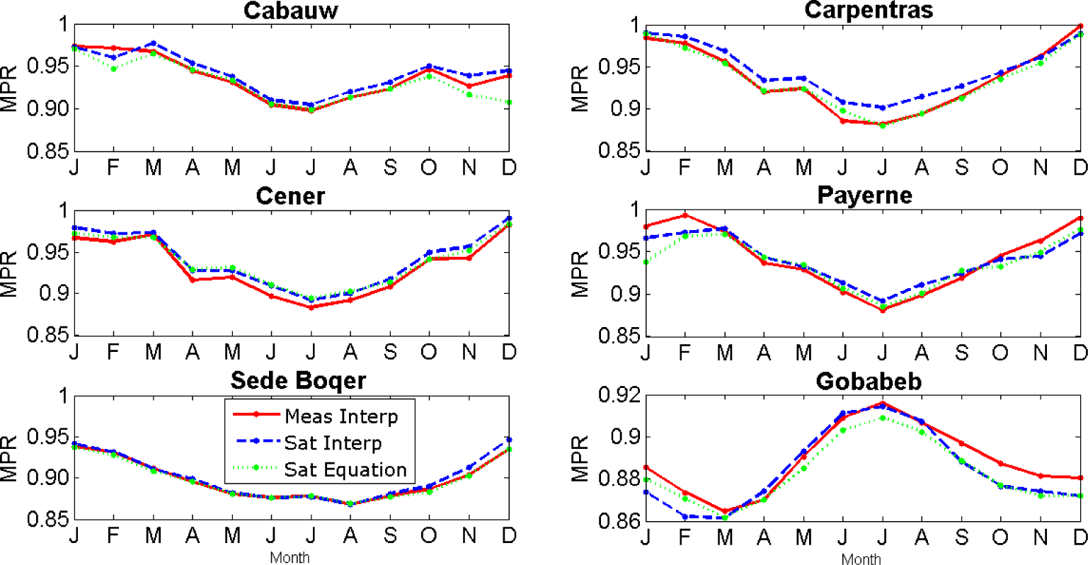
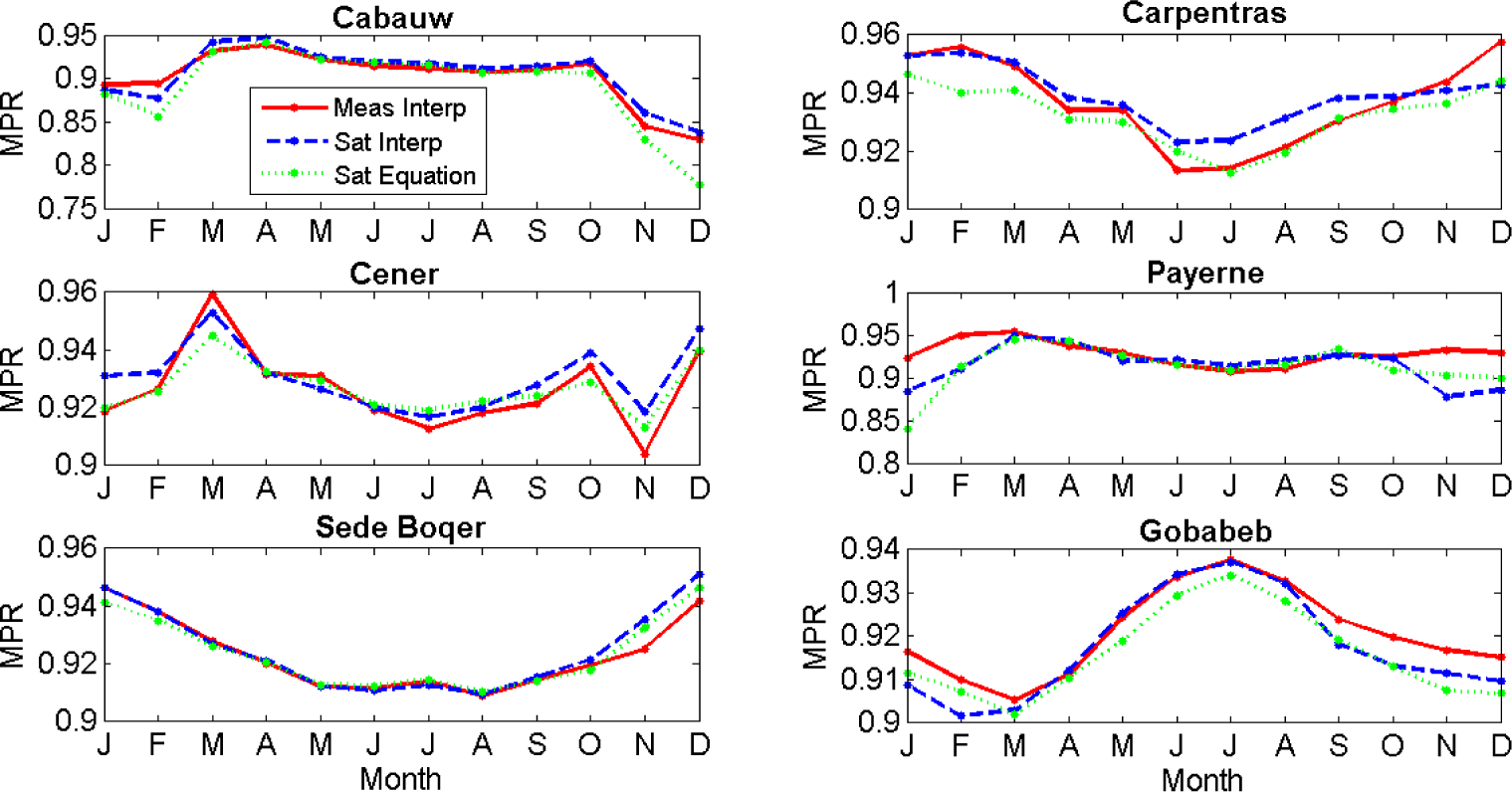
4.1. Comparison of PV Module Performance Using Measured and Satellite Retrieved Irradiance Data

There are, to our knowledge, no available data sets of direct measurements of PV module performance made on the same (or same model) modules in widely varying climates for a sufficient period of time to validate the entire chain of models described in Section 3. For this reason, a direct validation against experimental results is not possible, though each of the models used has been individually validated. We can, however, explore the effects of using different data sources for the irradiance and other meteorological data. To this end, we have performed calculations of MPR of two different module types for a number of different locations using different combinations of input data and two independent implementations of the models. In this section, the PV power output and the MPR have been calculated using satellite retrieved irradiance data and ground measurements recorded at the six BSRN stations shown in

Table 3. BSRN stations considered and year analyzed.

Location	Coordinates	Year
Cabauw (The Netherlands)	51.97° N, 4.93° E	2010
Carpentras (France)	44.08° N, 5.05° E	2010
Cener (Spain)	42.82° N, 1.60° W	2010
Payerne (Switzerland)	46.82° N, 6.95° E	2010
Sede Boqer (Israel)	30.87° N, 34.78° E	2010
Gobabeb (Namibia)	23.57° S, 15.01° E	2013

Therefore, two different data sets are considered, named “measured” and “satellite”, which contain the following variables required as input data:

• Global horizontal and direct horizontal irradiance values (GHI and DHI, respectively)
• Ambient temperature (T_amb)

Wind speed is not typically measured at the BSRN stations. Therefore the values for wind speed are common for both measured and satellite data sets and are derived from the operational forecast data provided by ECMWF. The ambient temperature values used in the satellite data set are also obtained from the ECMWF ERA-interim reanalysis with a correction for elevation differences [35]. In the measured data set, both irradiance values and the ambient temperature are the values registered at the BSRN station. Due to the lack of spectral irradiance measurements, the spectral effects are not taken into account in the estimation of the PV output.

Following the models described in Sections 3.1 and 3.2 it is possible to calculate the in-plane irradiance in the selected tilted plane (20° inclination regarding the horizontal plane and due south (north for Gobabeb station)) considering the AOI effects. With the estimated G_a values, the ambient temperature (T_amb) and the wind speed (W_ane), the module temperature (T_mod) is estimated following Equations (2) and (3).

The models described in Section 3 have been implemented both as a GRASS GIS module for calculations over large geographical areas, and independently as a MATLAB program (version R2015a) to calculate PV performance using time series of solar radiation and meteorological data for a single location. The two implementations are very similar but contain one difference: the GIS module uses Equation (4) directly with coefficients obtained from laboratory measurements on PV modules. In contrast, the single-location code uses an interpolation method to the values of a matrix containing the output power calculated according to Equation (4) for various combinations of module temperature and in-plane irradiance values. The module temperature varies between −15 to 85 °C in steps of 10 °C, while in-plane irradiance goes from 50 to 1200 W · m⁻² in 50 W · m⁻² intervals. When using the GRASS GIS module for the calculations, the PV output is estimated for very low and very high irradiance values, in opposition to the matrix, where those cases are not contemplated for the interpolation procedure.

In this section, two different PV technologies are studied: crystalline silicon and Cadmium Telluride. One matrix per technology is calculated using Equation (4) and the coefficients shown in Table 2. As a result, for every location and technology, there are three sets of PV output estimations:

• Measured–Single location: considering the data from the measured data set (measured irradiance and temperature values) and applying the interpolation method.
• Satellite–Single location: considering the data from the satellite data set (satellite retrieved irradiance values and ambient temperature from ECMWF ERA-interim reanalysis) and applying the interpolation method.
• Satellite–Equation: considering the data from the satellite data set together with temperature data from the ECMWF operational forecast and applying directly Equation (4).

For the first two procedures the moments when the sun elevation angle is below 5° are removed. In addition, the moments when the in-plane irradiance corrected for AOI effect is outside the range considered in the PV output matrix [50–1200 W · m⁻²] are removed as well. For the results obtained from the Equation (4) directly none of these criteria have been applied. The Module Performance Ratio is calculated according to Equation (7), for the whole year in the data set and per month. The yearly MPR values for both PV technologies and the three procedures applied are shown in

Table 4. Yearly Module Performance Ratio values.

MPR Station	Crystalline silicon			Cadmium Telluride
	Measured Interpolation	Satellite Interpolation	Satellite Equation	Measured Interpolation	Satellite Interpolation	Satellite Equation
Cabauw	0.926	0.933	0.926	0.915	0.921	0.913
Carpentras	0.923	0.936	0.921	0.932	0.937	0.928
Cener	0.921	0.929	0.928	0.926	0.929	0.927
Payerne	0.925	0.930	0.927	0.925	0.923	0.920
Sede Boqer	0.895	0.897	0.893	0.921	0.923	0.921
Gobabeb	0.888	0.883	0.882	0.920	0.917	0.915

.

The yearly values of the MPR are very similar in the three cases. Values derived from considering the model directly tend to be lower than those resulted from applying the interpolation method. CdTe has a slightly lower performance than c-Si modules for the first four stations. In contrast, for Sede Boqer and Gobabeb, the MPR is considerably higher for the CdTe technology. Analysing the monthly values of the MPR for these two stations we can see how the performance of CdTe technology is always higherr than the other technology. For the other stations, the c-Si technology shows higher MPR values during the winter months, while CdTe performs better during the summer months when both temperature and irradiance levels are higher. The monthly values of in-plane irradiance, ambient and module temperature used in the two procedures applying the interpolation method, as well as the resulting PV output and MPR, for the six locations are provided in the extra material [34].

Figure 1 shows for every location, the monthly values of MPR obtained from the three procedures for the c-Si technology.

The monthly values of MPR are also very similar with some exception for Cabauw and Payerne where in the winter months the MPR value from applying directly Equation (4) to the satellite values results in lower values. This may be due to the fact that in the interpolation procedure, moments with low in-plane irradiance were discarded, while in the map-based calculation times with very low irradiance were retained.

Similar behavior of the three procedures is observed for the CdTe technology. The three procedures provide very similar values. The monthly variability of the MPR values is in general higher for the c-Si technology than for the CdTe. The MPR for the c-Si varies within the year about 8%, while the variability for the CdTe is less than 6%.

The monthly variability of the MPR values is in general higher for the c-Si technology than for the CdTe. The MPR for the c-Si varies within the year about 8%, while the variability for the CdTe is less than 6%.

Figure 2 shows for every location, the monthly values of MPR obtained from the three procedures for the CdTe technology.

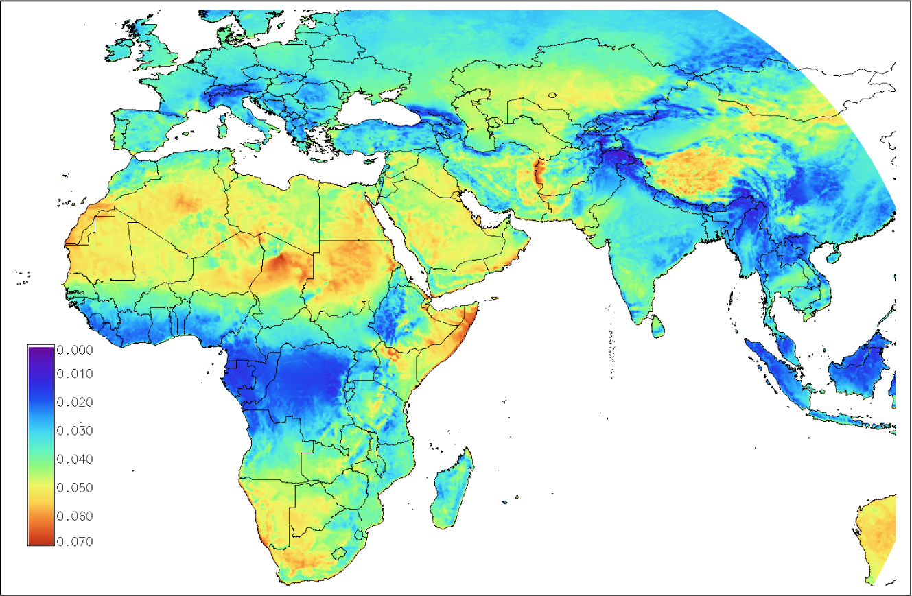
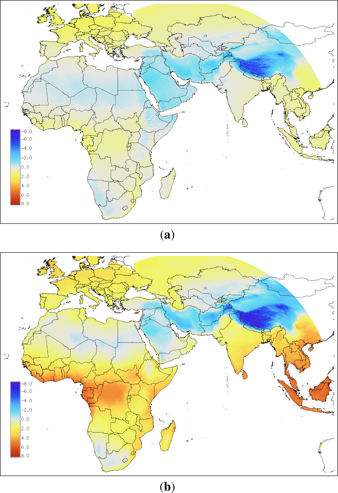
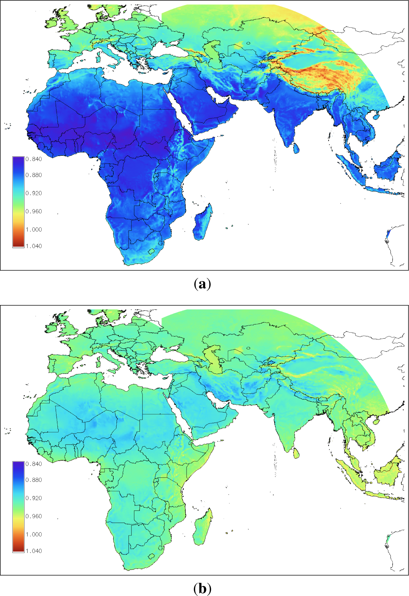
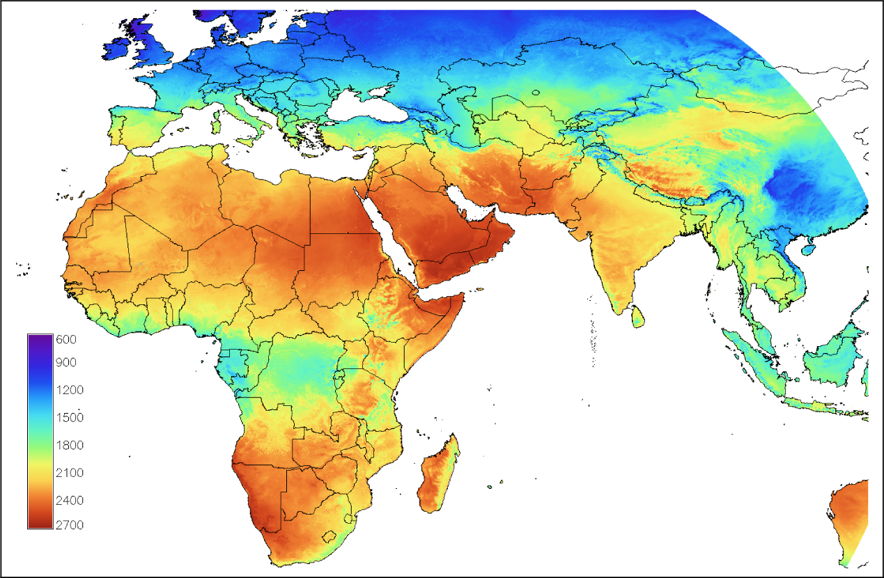
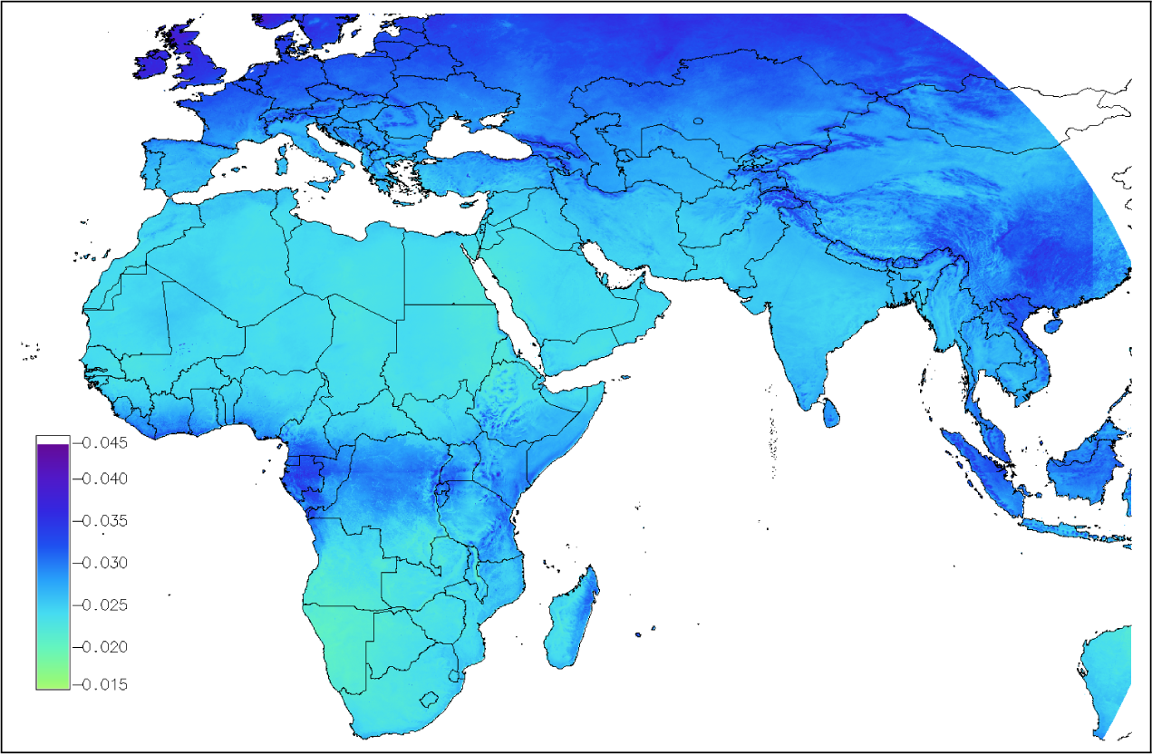
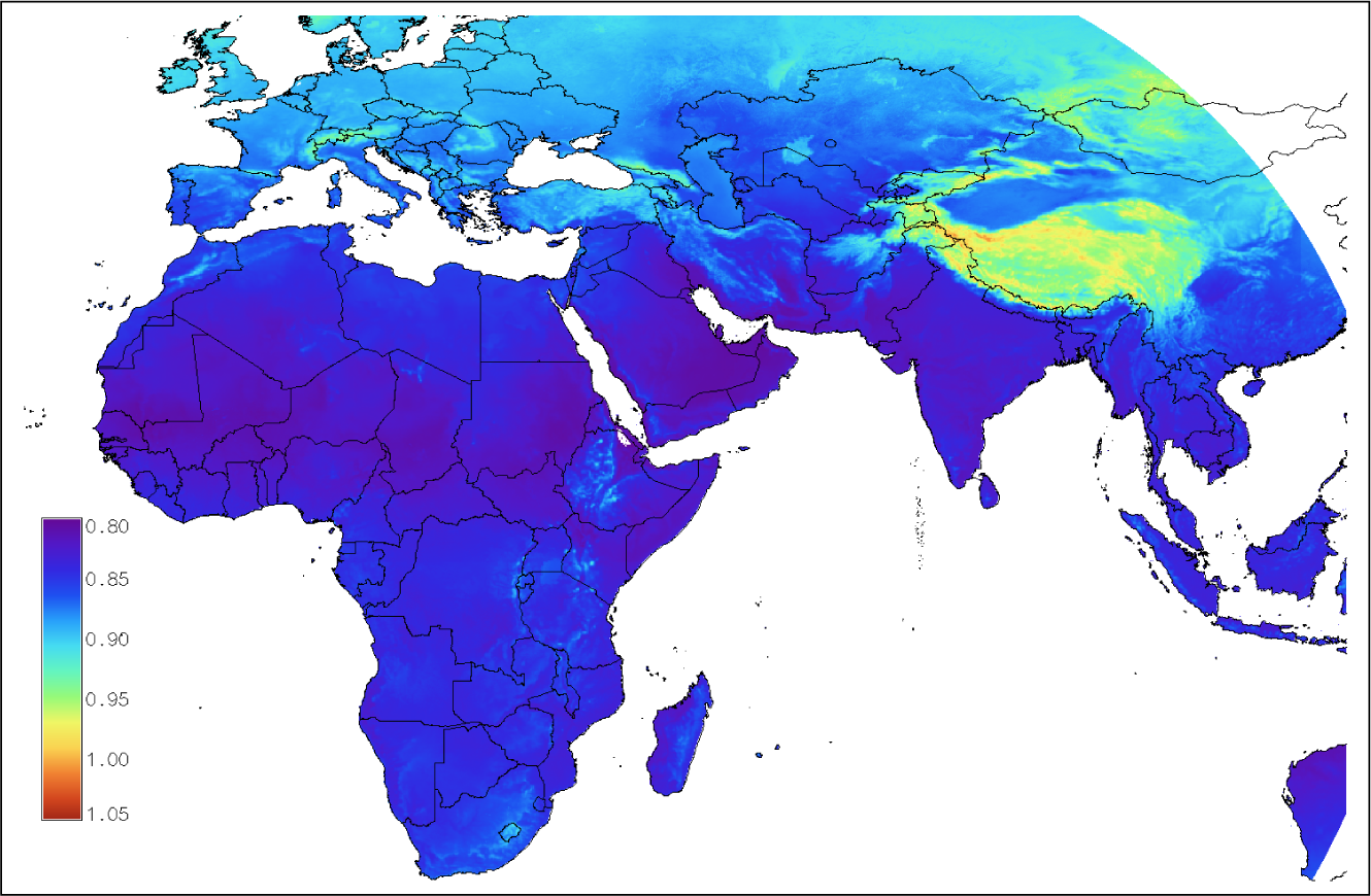
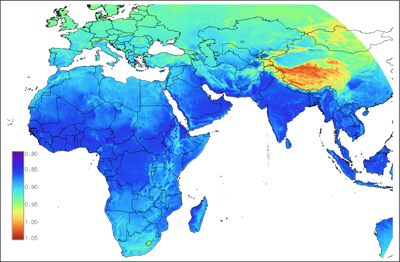
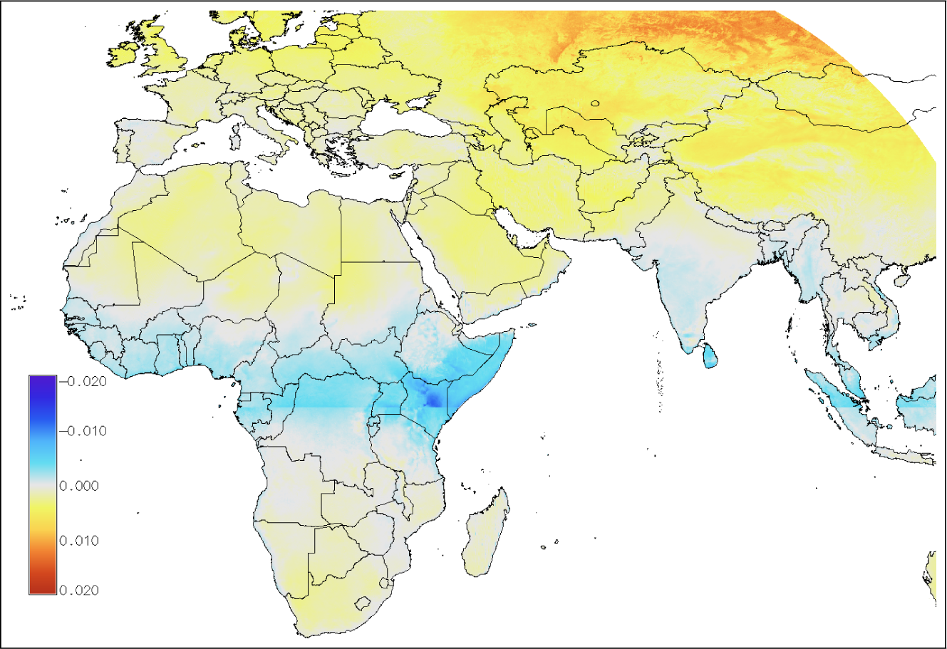
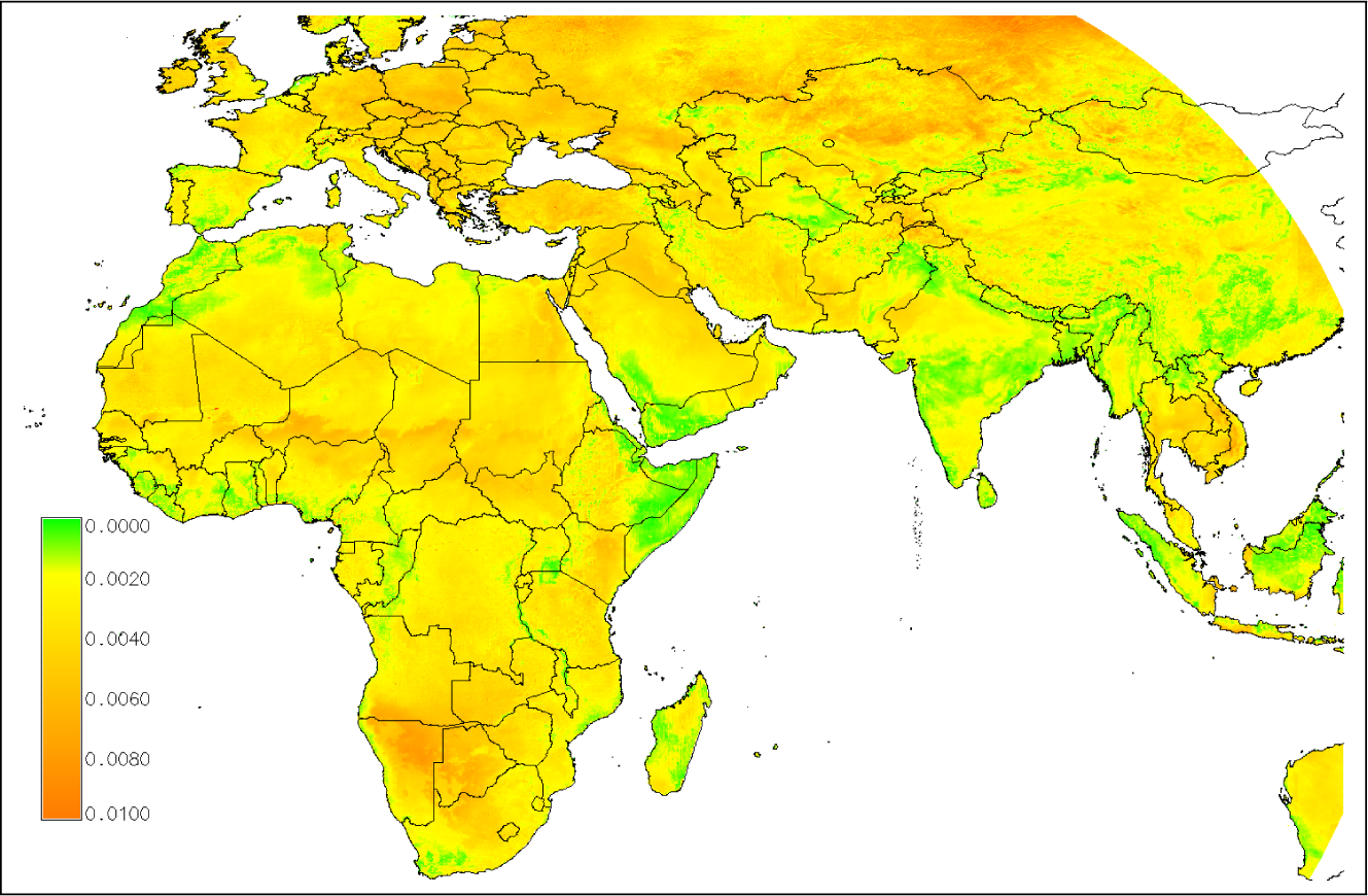
4.2. Calculations of PV Performance over Eurasia and Africa

Using the data described in Section 2.1 with the methods from Section 3.7 the calculations were performed for land surfaces in the area with the bounds:

• North: 60° N
• South: 40° S
• West: 25° W
• East: 115° E

The resulting total in-plane irradiation is shown as a map in Figure 3.

The geographical variation of the AOI effect is illustrated in Figure 4. This figure shows the relative difference between the calculations with and without the AOI model. The values range from about −0.015 to −0.045, meaning that the AOI effect will cause a decrease of irradiation entering the PV module that varies between 1.5% and 4.5%. A discontinuity is clearly seen at the equator because of the change in module orientation there. It is also clear that the effect is generally higher in more cloudy areas such as Tropical Africa, southern China and northern Europe. Note that in this calculation there is no distinction between different module types.

Based on the yearly totals of irradiation and PV output (calculated with and without wind), the MPR can be calculated according to Equation (7). The results are shown in Figures 5 and 6.

The variation in MPR follows a pattern that is very different from that seen in the irradiation map. Temperature has a very strong influence which can be seen in mountain areas such as the Caucasus and even more clearly in the Tibet high plateau.

The effects of wind are clearly seen and it is also clear that there is a strong geographical variation in this effect. For instance, the wind causes a noticeable increase in MPR in the Sahara, while in the Congo basin the effect is much smaller. Figure 7 shows the difference in MPR with or without the effect of wind on the module temperature. Generally, the effect is strong in The Sahara and Kalahari deserts, in the Tibet plateau and in Kazakhstan, moderate in most of Europe, and quite weak in Tropical Africa, east Asia and Southern China. In extreme cases the effect can reach more than 6%.

4.3. The Effect of Module Inclination on Module Performance Ratio

All the results shown so far have used a single fixed module inclination of 20°. If a different inclination angle is chosen, this will change the in-plane irradiance at any given moment and so change the module efficiency both because of the change in irradiance and because the module temperature will change.

In principle, the relation shown in Equation (3) would be expected to change somewhat with the module’s inclination angle, and the effect of cooling by wind may be more effective at steeper module inclinations. However, the model data available do not distinguish between module inclinations, so this will not be taken into account.

The effect of module inclination on MPR was investigated by repeating the above calculations with a module inclination of 40° with modules still facing equator. Considering all the effects (AOI, air temperature, wind speed) we then calculated the difference in MPR between the two scenarios. The resulting map is shown in Figure 8. The results show that there are clear geographical patterns with a positive difference (MPR is higher at 40°) in southern Siberia and a negative difference near the equator. However, the absolute value of the difference is small. In most areas (Europe, South Asia, most of Africa, China) the absolute value of the difference is well below 0.5%. Only in extreme cases (southern Siberia, equatorial East Africa) does the difference approach ±1%. This should be compared to overall differences in MPR of up to 20% between locations in the study area (see Figure 6). The result is consistent with that found in Huld et al., 2008 [2], where the performance of fixed-mounted and 2-axis tracking systems were compared and it was found that the relative difference in PV energy yield was almost the same whether or not irradiance and temperature effects were taken into account.

4.4. Interannual Variation in MPR

The results presented above have been calculated using hourly data (irradiance, temperature and wind speed) for a single year (2011). For a given location, the average temperature will vary from year to year, and the total irradiation may also vary by several percent from one year to the next. It is therefore not a given that the average MPR for a single year will be representative of other years. To investigate this, we performed the calculations of MPR taking into account AOI, temperature and wind speed for a total of 4 years, 2010–2013, which is the period for which the high-resolution temperature and wind data are available. From the values of H and E_w the average MPR was calculated for each of the four years and the standard deviation of the annual average MPR was calculated for each point in the geographical region. The map of the standard deviation of MPR is shown in Figure 9. The standard deviation is everywhere less than 0.01 and in most areas less than 0.005. Using a Student t distribution with 3 degrees of freedom, the probability of average MPR for a given year deviating by more than 0.025 from the 4-year mean is less than 5% everywhere and in most areas there is less than 5% probability of the MPR in a given year deviating by more than 0.012. This should be compared with the overall variation in MPR which exceeds 0.2. The maps of MPR using one year of data are therefore quite representative of the average MPR over long time periods. Of course, the actual energy yield of a PV system will vary much more strongly from year to year as the annual irradiation varies.

4.5. Influence of Module Type

The results presented in Subsections 4.2 to 4.4 have only considered crystalline silicon modules. Different PV cell technologies may give different overall MPR values because of difference in the behavior at low light intensity or high temperature.

To illustrate this difference we have repeated the calculations of annual average MPR also for a Cadmium Telluride module. For this module type the coefficients for the model of Equation (4) are given in Table 2. In order to compare the performance of CdTe modules with c-Si modules of the same nominal power, we then calculated the relative difference in MPR between the two module types. The resulting map is shown in Figure 10. In areas with positive values in this map, CdTe modules will have higher annual energy output, whereas when the difference is negative, c-Si modules will have higher energy output. The results shown in Figure 10 agree with the values of MPR presented in Table 4.

4.6. Effect of Spectral Variation on the Energy Output of Different Module Types

The preceding results have not considered the effect of variations in the solar spectrum. The model to include this effect was introduced in Subsection 3.3. The resulting effective irradiance G_eff (Equation (1)) can then be used with Equation (4) to calculate the spectrally corrected PV power. Note that the irradiance input to Equation (3) should be the uncorrected irradiance.

The calculation of total PV energy including spectral effects was performed for the year 2013. The PV energy output was also calculated for the same year without considering spectral effects. The influence of spectral variations can then be illustrated by calculating the difference between these two results. The result is shown in Figure 11. In most areas the effect of spectral variations is not the dominant effect though the effect is not negligible. Generally, the effect is stronger for CdTe than for c-Si. As shown in [11], the spectral effect is generally stronger for PV technologies with a more narrow spectral range. An exception to this trend is found in the high-elevation areas in Asia, in particular Tibet, where the two technologies show a marked negative influence of the spectral effect. A possible explanation for this could be that in these high-elevation and low temperature areas the air has a very low water vapor content. This could allow a higher proportion of infrared radiation to arrive at ground level. Since this infrared radiation is not used by the PV modules, the overall effect will be a reduced PV power relative to the broadband irradiance.

In [11] a comparison was made between the present method and results of other researchers [9,10] and it was shown that the results agree well. In this work the calculation of the spectral effects have been extended to Asia and we can therefore now make a comparison also with the results of Ye et al. [8]. For CdTe we estimate an overall yearly energy gain of +5% while the results from [8] show about +3%. It should be noted that the results are not directly comparable since our calculation is based on the full calculation of the PV power including temperature effects while other researchers have based the calculation on the variation in the short-circuit current.

4.7. Combining All Models

Once the total PV energy output has been calculated using the models for all the effects discussed here, we can calculate the overall module performance ratio.

These results are effectively a combination of the data shown in Figure 6 with those of Figure 11. The resulting maps are shown in Figure 12.

5. Conclusions and Further Work

We have presented results of a study of the geographical variation of several effects that influence the performance of PV systems:

• PV module reflectivity at shallow angles of incidence (angle-of-incidence effect)
• Effects of variation in the solar spectrum
• Dependence of module efficiency on in-plane irradiance and module temperature
• Effects of irradiance, air temperature and wind speed on the module temperature

Using published models for these effects we have been able to calculate their magnitude over an area covering Europe, Africa and nearly all of Asia. Some of these effects are fairly homogeneous over the studied area while others vary much more strongly. Thus, the overall size of the angle-of-incidence effect is in the range −2% to −4%. The effect of variations in the spectrum shows a greater range in magnitude. For crystalline silicon modules this will range from −5% to +2% while the effect is more pronounced for CdTe modules, varying from −6% to +6%.

The greatest effect is found in the dependence of module efficiency on temperature and irradiance. For crystalline silicon, this effect may vary from −15% to +5% depending on location, while CdTe modules show somewhat less geographical variation, mainly due to the smaller temperature coefficient. The cooling effect of wind may change the overall module performance ratio by 5% or more in hot, windy areas such as the Sahara desert.

The study presented here includes several of the most important effects influencing PV performance. However, the study may be refined in a number of ways:

• Some new PV module types have special coatings or textured surfaces to reduce the losses due to reflectivity. Measured data from such modules could be used to quantify the improvement in overall PV energy output.
• The method for estimating the spectral effects has so far only considered single-junction PV technologies. Tandem cells and multijunction technologies will require modifications to the methods used here.
• Some PV technologies show long-term variation in the module efficiency. This is especially the case for amorphous silicon technologies. This will require development of models for the behaviour of these modules.
• PV module performance tends to degrade with age, in a way that almost certainly depends on the environmental conditions. Better models for this effect will have to be developed before it is possible to estimate the geographical variation of age-related degradation.

The data used to produce the geospatial maps in this paper can be downloaded from re.jrc.ec.europa.eu/pvgis/energy_rating_paper/index.html.

References

1. Martin, N.; Ruiz, J. Calculation of the PV modules angular losses under field conditions by means of an analytical model. Solar Energy Mater. Solar Cells 2001, 70, 25–38. [Google Scholar]
2. Huld, T.; Šúri, M.; Dunlop, E. Comparison of potential solar electricity output from fixed-inclined and two-axis tracking photovoltaic modules in Europe. Prog. Photovolt. Res. Appl. 2008, 16, 47–59. [Google Scholar]
3. Huld, T.; Gottschalg, R.; Beyer, H.; Topič, M. Mapping the performance of PV modules, effects of module type and data averaging. Solar Energy 2010, 84, 324–338. [Google Scholar]
4. Gottschalg, R.; Infield, D.G.; Kearny, M.J. Experimental study of variations of the solar spectrum of relevance to thin film solar cells. Solar Energy Mater. Solar Cells 2003, 79, 527–537. [Google Scholar]
5. Gottschalg, R.; Betts, T.R.; Williams, S.R.; Sauter, D.; Infield, D.G.; Kearny, M.J. A critical appraisal of the factors affecting energy production from amorphous silicon photovoltaic arrays in a maritime climate. Solar Energy 2004, 77, 909–916. [Google Scholar]
6. Minemoto, T.; Nagae, S.; Takakura, H. Impact of spectral irradiance distribution and temperature on the outdoor performance of amorphous Si photovoltaic modules. Solar Energy Mater. Solar Cells 2007, 91, 919–923. [Google Scholar]
7. Cornaro, C.; Andreotti, A. Influence of average photon energy index on solar irradiance characteristics and outdoor performance of photovoltaic modules. Progress Photovolt. Res. Appl. 2013, 21, 996–1003. [Google Scholar]
8. Ye, J.Y.; Reindl, T.; Aberle, A.G.; Walsh, T.M. Effect of solar spectrum on the performance of various thin-film PV module technologies in tropical Singapore. IEEE J. Photovolt. 2014, 4, 1268–1274. [Google Scholar]
9. Alonso-Abella, M.; Chenlo, F.; Nofuentes, G.; Torres-Ramirez, M. Analysis of spectral effects on the energy yield of different PV (photovoltaic) technologies: The case of four specific sites. Energy 2014, 67, 435–443. [Google Scholar]
10. Dirnberger, D.; Blackburn, G.; Müller, B.; Reise, C. On the impact of solar spectral irradiance on the yield of different PV technologies. Solar Energy Mater. Solar Cells 2015, 132, 431–442. [Google Scholar]
11. Gracia Amillo, A.; Huld, T.; Vourlioti, P.; Müller, R.; Norton, M. Application of satellite-based spectrally resolved solar radiation data to PV performance studies. Energies 2015, 8, 3455–3488. [Google Scholar]
12. Skoplaki, E.; Palyvos, J. On the temperature dependence of photovoltaic module electrical performance: A review of efficiency/power correlations. Solar Energy Mater. Solar Cells 2009, 83, 614–624. [Google Scholar]
13. Faiman, D. Assessing the outdoor operating temperature of photovoltaic modules. Prog. Photovolt. Res. Appl. 2008, 16, 307–315. [Google Scholar]
14. Koehl, M.; Heck, M.; Wiesmeier, S.; Wirth, J. Modeling of the nominal operating cell temperature based on outdoor weathering. Solar Energy Mater. Solar Cells 2011, 95, 1638–1646. [Google Scholar]
15. King, D.; Boyson, W.; Kratochvil, J. Photovoltaic Array Performance Model; Technical Report SAND2004-3535; Sandia National Laboratories: Albuquerque, NM, USA, 2004. [Google Scholar]
16. Dittmann, S.; Friesen, G.; Williams, S.; Betts, T.; Gottschalg, R.; Beyer, H.; Guérin de Montgareuil, A.; van der Borg, N.; Burgers, A.; Huld, T.; et al. Results of the 3rd modeling round robin within the European project PERFORMANCE—Comparison of module energy rating methods, Proceedings of the 25th European Photovoltaic Solar Energy Conference, Valencia, Spain, 6–10 September 2010; pp. 4333–4338.
17. Huld, T.A.; Friesen, G.; Skoczek, A.; Kenny, R.A.; Sample, T.; Field, M.; Dunlop, E.D. A power-rating model for crystalline silicon PV modules. Solar Energy Mater. Solar Cells 2011, 95, 3359–3369. [Google Scholar]
18. IEC Central Office. Photovoltaic Devices—Part 3: Measurement Principles for Terrestrial Photovoltaic (PV) Solar Devices with Reference Spectral Irradiance Data; Technical Report IEC 61215-3; International Electrotechnical Commission: Geneva, Switzerland, 2005. [Google Scholar]
19. Bücher, K. Site dependence of the energy collection of PV modules. Solar Energy Mater. Solar Cells 1997, 47, 85–94. [Google Scholar]
20. Agugiaro, G.; Nex, F.; Remondino, F.; de Filippi, R.; Droghetti, S.; Furlanello, C. Solar radiation estimation on building roofs and web-based solar cadastre, Proceedings of the ISPRS Annals of the Photogrammetry, Remote Sensing and Spatial Information Sciences, Melbourne, Australia, 25 August–1 September 2012; pp. 177–182.
21. Ramirez Camargo, L.; Zink, R.; Dorner, W.; Stoeglehner, G. Spatio-temporal modeling of roof-top photovoltaic panels for improved technical potential assessment and electricity peak load offsetting at the municipal scale. Comput. Environ. Urban Syst. 2015, 52, 58–69. [Google Scholar]
22. Nguyen, H.; Pearce, J. Estimating potential photovoltaic yield with r.sun and the open source Geographical Resources Analysis Support System. Solar Energy 2010, 84, 831–843. [Google Scholar]
23. Huld, T.; Šúri, M.; Dunlop, E. Geographical variation of the conversion efficiency of crystalline silicon photovoltaic modules in Europe. Prog. Photovolt. Res. Appl. 2008, 16, 595–607. [Google Scholar]
24. Müller, R.; Matsoukas, C.; Gratzki, A.; Behr, H.; Hollmann, R. The CM-SAF operational scheme for the satellite based retrieval of solar surface irradiance—A LUT based eigenvector hybrid approach. Remote Sens. Environ. 2009, 113, 1012–1024. [Google Scholar]
25. Huld, T.; Müller, R.; Gambardella, A. A new solar radiation database for estimating PV performance in Europe and Africa. Solar Energy 2012, 86, 1803–1815. [Google Scholar]
26. Müller, R.; Behrendt, T.; Hammer, A.; Kemper, A. A new algorithm for the satellite-based retrieval of solar surface irradiance in spectral bands. Remote Sens. 2012, 4, 622–647. [Google Scholar]
27. Gracia Amillo, A.; Huld, T.; Müller, R. A new database of global and direct solar radiation using the eastern meteosat satellite, models and validation. Remote Sens. 2014, 6, 8165–8189. [Google Scholar]
28. Muneer, T. Solar radiation model for Europe. Build. Serv. Eng. Res. Technol. 1990, 4, 153–163. [Google Scholar]
29. Gracia Amillo, A.; Huld, T. Performance Comparison of Different Models for the Estimation of Global Irradiance on Inclined Surfaces; Technical Report; European Commission Joint Research Centre. Avaliable online: http://re.jrc.ec.europa.eu/pvgis/doc/report/ReqNO_JRC81902_Report.pdf accessed on 20 March 2015.
30. IEC Central Office. Crystalline Silicon Terrestrial Photovoltaic (PV) Modules—Design Qualification and Type Approval; Technical Report IEC-60904-3; International Electrotechnical Commission: Geneva, Switzerland, 2008. [Google Scholar]
31. Bahrs, U.; Zaaiman, W.; Mertens, M.; Ossenbrink, H. Automatic large area spectral response facility, Proceedings of the 14th European Photovoltaic Solar Energy Conference, Barcelona, Spain, 30 June–4 July 1997; pp. 2296–2298.
32. Nikolaeva-Dimitrova, M.; Kenny, R.; Dunlop, E.; Pravettoni, M. Seasonal variations on energy yield of a-Si, hybrid, and crystalline Si PV modules. Prog. Photovolt. Res. Appl. 2010, 14, 311–320. [Google Scholar]
33. Piliougine, M.; Elizondo, D.; Mora-López, L.; Sidrach-de Cardone, M. Multilayer perceptron applied to the estimation of the influence of the solar spectral distribution on thin-film photovoltaic modules. Applied Energy 2013, 112, 610–617. [Google Scholar]
34. Huld, T.; Gracia Amillo, A.M. Supplementary material for the present paper. Availiable online: http://re.jrc.ec.europa.eu/pvgis/papers_supplementary/performance_mapping/index.html accessed on 20 May 2015.
35. Huld, T.; Pinedo Pascua, I. Spatial downscaling of 2-meter air temperature using operational forecast data. Energies 2015, 8, 2381–2411. [Google Scholar]
Figure 1. Monthly MPR values for the c-Si technology.
Energies 08 05159f1
Figure 2. Monthly MPR values for the CdTe technology.
Energies 08 05159f2
Figure 3. Total in-plane solar irradiation for an equator-facing plane inclined 20° from horizontal. The result is given in units of kWh·m2.
Energies 08 05159f3
Figure 4. Relative difference between total irradiation calculated with and without the AOI effects.
Energies 08 05159f4
Figure 5. Module performance ratio for crystalline silicon modules, taking into account the effects of temperature and low irradiance but NOT the effects of wind.
Energies 08 05159f5
Figure 6. Module performance ratio for crystalline silicon modules, taking into account the effects of temperature and low irradiance as well as the effects of wind.
Energies 08 05159f6
Figure 7. Difference between the MPR values calculated with or without taking into account the effect of wind.
Energies 08 05159f7
Figure 8. Difference between the MPR values for modules at 40° and 20° inclination (free rack mounted facing equator).
Energies 08 05159f8
Figure 9. Standard deviation in annual MPR values taking into account 4 years from 2010 to 2013.
Energies 08 05159f9
Figure 10. Relative difference in MPR values between CdTe modules and c-Si modules.
Energies 08 05159f10
Figure 11. Relative difference (in %) in total energy production when taking spectral effects into account compared to the same calculation where the spectrum is assumed to be always proportional to the STC spectrum. (a) Results for c-Si (b) Results for CdTe.
Energies 08 05159f11
Figure 12. Module performance ratio taking into account AOI, spectral effects, and the effects of temperature and irradiance on PV power. (a) c-Si modules; (b) CdTe modules.
Energies 08 05159f12