Empirical Research on China’s Carbon Productivity Decomposition Model Based on Multi-Dimensional Factors

Abstract

Based on the international community’s analysis of the present CO₂ emissions situation, a Log Mean Divisia Index (LMDI) decomposition model is proposed in this paper, aiming to reflect the decomposition of carbon productivity. The model is designed by analyzing the factors that affect carbon productivity. China’s contribution to carbon productivity is analyzed from the dimensions of influencing factors, regional structure and industrial structure. It comes to the conclusions that: (a) economic output, the provincial carbon productivity and energy structure are the most influential factors, which are consistent with China’s current actual policy; (b) the distribution patterns of economic output, carbon productivity and energy structure in different regions have nothing to do with the Chinese traditional sense of the regional economic development patterns; (c) considering the regional protectionism, regional actual situation need to be considered at the same time; (d) in the study of the industrial structure, the contribution value of industry is the most prominent factor for China’s carbon productivity, while the industrial restructuring has not been done well enough.

1. Introduction

CO₂ emissions have become a major global issue with common concern by the international community. This emission issue influences not only the global ecological environment but also the global economy, which is closely linked with the production and life of mankind [1]. Under the trend of development of the world economy, most developing countries regard economic growth as their single target. The investigation of significant resources and the extensive growth mode as well as the human activities have produced large quantities of CO₂ that directly lead to low economic benefits, environmental pollution and other problems. Therefore, how to arrange energy consumption properly [2] and minimize the impact of human activities on the ecological environment [3] have drawn increasing attention of the international community.

Jointly established by the World Meteorological Organization (WMO) and the United Nations Environment Programme (UNEP) in 1984, the Intergovernmental Panel on Climate Change (IPCC) is responsible for assessing the scientific information on climate change and evaluating environmental and socio-economic consequences caused by climate change. Held in Durban of South Africa in 2011, the 17th Conference of the Parties (COP17) to the United Nations Framework Convention on Climate Change (UNFCCC)/the 7th Conference of the Parties to The Kyoto Protocol (CMP7) established the decision “to strengthen action ‘Durban Platform’ Ad Hoc Working Group”. In November 2013, the UNFCCC COP 19/CMP9 was held in Warsaw, Poland. The focus of the Warsaw talks is still concentrated on the “Durban Platform”. In addition, the Warsaw talks covered the “green development fund” that developed countries should create to provide financial support, technology transfer and capacity building for developing countries to address climate change.

Although the international community is paying more and more attention to CO₂ emissions, fossil energy will still be irreplaceable for economic development in the near future considering the speed and degree of new energy research and development [4]. At the same time, due to the limits of technology and costs, carbon capture technology and carbon recycling technology are still difficult to apply widely in the short term [5]. Therefore, CO₂ emissions caused by the consumption of fossil fuels cannot be avoided. In this case, improving the efficiency of CO₂ emissions is the only way to coordinate the relationships between economic development, energy consumption and CO₂ emissions and thus realize sustainable development of human society.

The growth of carbon emissions caused by the increase of fossil fuel consumption is mainly attributed to the increase of GDP. Therefore, it’s particularly necessary to choose a universally recognized economic indicator to assess the carbon intensity of a country or a region so that the responsibility each region should bear is clarified according to different levels of carbon emissions. In this context, the Japanese energy economists Kaya and Yokobori [6] first proposed the concept of carbon productivity, defining the carbon productivity as ratio of GDP output and CO₂ emissions. After that, the US Energy Information Administration defined the reciprocal carbon productivity as carbon density and regards it as one of the indicators to reflect the level of greenhouse gas emissions [7]. In 2010, He and other scholars have pointed out that changes in the country’s carbon productivity can be an important indicator to measure global climate change [8]. This view has received global recognition from a majority of scholars [9,10,11]. In addition, considering the differences between the CO₂ emissions of different regions, carbon productivity may perfectly determine the CO₂ emission reduction numbers according to the actual level of economic development. Therefore, it is really necessary to quantitatively decompose the carbon productivity of a country into various influential factors and different industrial structures in different regions.

Currently, the Log Mean Divisia Index (LMDI) [12,13,14] and Laspeyre [15,16,17,18] are the two most widely used kinds of decomposition algorithms in energy consumption studies. These two algorithms reflect changes in energy consumption by different quantified factors. The LMDI decomposition algorithm is applied as the basic algorithm in this paper for its good capabilities in analysis and interpretation and the ability to do comprehensive analysis using data of different industrial structures, different regions and different kinds of energy.

The LMDI index decomposition method has been widely used for the decomposition of energy consumption and CO₂ emissions since this method was introduced to the energy decomposition field. For example, Ang et al. [19] and Wang et al. [20] applied the LMDI decomposition method and discovered that economic growth is a major source of CO₂ emissions. Lin et al. [21] analyzed the factors affecting the demand of fossil fuels in a similar way and estimated the potential fossil fuel savings. By the similar method Xu et al. [22] decomposed the carbon emissions into energy intensity, energy structure, industrial structure, economic output and population size, based on the value of the energy consumption. They concluded that economic output is the main driver of carbon emissions, followed by population size and energy structure, and that energy intensity of carbon emissions is the major inhibiting factor in carbon emissions. Xu et al. [23] used CO₂ emission data from 1996 to 2011 in China, combined with energy policy and the implementation of initiatives, and reached the conclusions that economic growth was the main driving factor and lower energy intensity would inhibit the increase of CO₂ emissions. Zhou et al. [24] analyzed the energy efficiency of China’s seven regions and CO₂ emissions produced due to thermoelectric power generation. Their result provides a theoretical basis for encouraging the construction of great power plants and limiting small power plants in China. Gonzalez et al. [25] generated Monetary Based (MB), Intensity Refactorization (IR) and Activity Revaluation (AR) analytical methods based on the LMDI decomposition method, and applied them in the analysis of CO₂ emissions from the power sector in Europe. Holzman et al. [26] explored the reason why the final energy does not decline as expected and found that residents’ increased demand for comfort offsets the fruit of energy consumption reduction through technology improvement. Balezentis [27] analyzed the factors affecting the Lithuanian energy intensity. Li et al. [28] estimated the amount of CO₂ emissions in 1994–2011 and decomposed the carbon emissions. The results showed that agricultural subsidies play a vital role in reducing CO₂ emissions. Vaninsky [29] expanded the Cara identity and compared the differences in carbon emissions between the US and China from GDP, energy consumption carbon intensity and population. Shao [30] analyzed the time series of carbon emissions from the energy consumption of the industrial sector and divided industries into different types and analyzed combination features of “emissions-efficiency”.

The above studies mainly focused on using of LMDI decomposition model for carbon emissions and energy consumption. However, there is little research if any on the decomposition of carbon productivity from the current research status, and those studies only took part of the industrial structure and energy class into consideration or it just did analysis considering one dimension or two. It is difficult for such a result to fully reflect changes in a country or region’s carbon productivity. Based on the studies above, this article describes the subdivision of the factors influencing the carbon productivity and on the basis of the industrial structure and regional decomposition, the multidimensional factors, and a combined application of the LMDI decomposition model are established. As these three dimensions are independent from each other, the analysis on carbon productivity changes can be comprehensive and this model can also explain the deeper reasons behind the changes.

This paper is structured as follows: Section 2 describes the decomposition of the carbon productivity model based on LMDI; Section 3 introduces the data sources; Section 4 describes the specific decomposition of results; Section 5 discusses the factors influencing carbon productivity contributions from three dimensions—factors, region and industry structure—as well as the causes of the contribution value differences; Section 6 is the conclusion of this paper and gives some policy recommendations.

2. Material and Models

2.1. Decomposition Model of Carbon Productivity

According to the definition of carbon productivity, carbon productivity equation can be represented as:

$$P=\frac{Y}{C}=\frac{{\displaystyle \sum Y}}{C}$$

(1)

where P denotes carbon productivity, Y indicates the GDP of a country, and C is the CO₂ emissions. In order to reflect the relationship among carbon productivity, industrial structure, and regional as well as the influencing factors, the above formula needed to be extended as:

$$P=\frac{Y}{C}=\frac{{\displaystyle \sum Y}}{C}=\frac{{\displaystyle \sum _i{\displaystyle \sum _j{Y}_{ij}}}}{C}=\frac{{\displaystyle \sum _i{\displaystyle \sum _j\frac{Y_{ij}}{C_{ij}}\cdot \frac{C_{ij}}{E_{ij}}\cdot \frac{E_{ij}}{E_i}\cdot \frac{E_i}{Y_i}\cdot \frac{Y_i}{P_i}\cdot \frac{P_i}{P}\cdot p}}}{C}$$

(2)

where Y_ij denotes the GDP from industrial activity j of region i, C_ij is the CO₂ emissions from industry j of region i, E_ij denotes the energy consumption from industry j of region i, E_i denotes the energy consumption from region i, Y_i denotes GDP in the region i, P_i denotes the population in region i, P denotes the population in the country. Based on the above formula, the influencing factors of carbon productivity can be decomposed into industrial actual carbon productivity in the area ($\Delta (Y_{ij}/C_{ij})$) which is represented by $P_{ij}$, carbon intensity ($\Delta (C_{ij}/E_{ij})$) which is represented by $C{I}_{ij}$, energy structure ($\Delta (E_{ij}/E_i)$) which is represented by $E{S}_{ij}$, energy intensity ($\Delta (E_i/Y_i)$) which is represented by $E{I}_i$, economic output ($\Delta (Y_i/P_i)$) which is represented by $PC{G}_i$, population scale ($\Delta (P_i/P)$) which is represented by $P{S}_i$, and the reciprocal of per capita carbon emissions ($\Delta (P/C)$), which is represented by $PC$.

2.2. Complete Decomposition Model

Based on the above decomposition model, we cannot analyze various factors on the carbon productivity contribution quantitatively, so the decomposition model needs to be further refined. When introducing time (t) into Equation (2) and its differential, the equation is written as:

$$\frac{d{P}_t}{dt}={\displaystyle \sum _{i=1}^n{\displaystyle \sum _{j=1}^n\frac{d(\frac{Y_{ijt}}{C_{ijt}})}{dt}}}\cdot \frac{C_{ijt}}{C_t}+{\displaystyle \sum _{i=1}^n{\displaystyle \sum _{j=1}^n\frac{d(\frac{C_{ijt}}{E_{ijt}})}{dt}}}\cdot \frac{Y_{ijt}}{C_{ijt}}\cdot \frac{E_{ijt}}{C_t}+{\displaystyle \sum _{i=1}^n{\displaystyle \sum _{j=1}^n\frac{d(\frac{E_{ijt}}{E_{it}})}{dt}}}\cdot \frac{Y_{ijt}}{C_t}\cdot \frac{E_{it}}{E_{ijt}}+{\displaystyle \sum _{i=1}^n{\displaystyle \sum _{j=1}^n\frac{d(\frac{E_{it}}{Y_{it}})}{dt}}}\cdot \frac{Y_{ijt}}{E_{it}}\cdot \frac{Y_{it}}{C_t}+{\displaystyle \sum _{i=1}^n{\displaystyle \sum _{j=1}^n\frac{d(\frac{Y_{it}}{P_{it}})}{dt}}}\cdot \frac{Y_{ijt}}{Y_{it}}\cdot \frac{P_{it}}{C_t}+{\displaystyle \sum _{i=1}^n{\displaystyle \sum _{j=1}^n\frac{d(\frac{P_{it}}{P_t})}{dt}}}\cdot \frac{Y_{ijt}}{C_t}\cdot \frac{P_t}{C_{it}}+{\displaystyle \sum _{i=1}^n{\displaystyle \sum _{j=1}^n\frac{d(\frac{P_t}{C_t})}{dt}}}\cdot \frac{Y_{ijt}}{P_t}$$

(3)

Equation (3) shows the differential of P_t. Hence its definite integral will reflect the variation result of P_t between two time points. Since z and u are two different statistical time points (z > u), the definite integral of Equation (3) from u to z is:

$$P_z-P_u={\displaystyle \sum _{i=1}^n{\displaystyle \sum _{j=1}^n{\displaystyle {\int }_u^z\frac{C_{ijt}}{C_t}}}}\cdot \frac{d(\frac{Y_{ijt}}{C_{ijt}})}{dt}dt+{\displaystyle \sum _{i=1}^n{\displaystyle \sum _{j=1}^n{\displaystyle {\int }_u^z\frac{Y_{ijt}}{C_{ijt}}}}}\cdot \frac{E_{ijt}}{C_t}\cdot \frac{d(\frac{C_{ijt}}{E_{ijt}})}{dt}dt+{\displaystyle \sum _{i=1}^n{\displaystyle \sum _{j=1}^n{\displaystyle {\int }_u^z\frac{Y_{ijt}}{C_t}}}}\cdot \frac{E_{it}}{E_{ijt}}\cdot \frac{d(\frac{E_{ijt}}{E_{it}})}{dt}dt+{\displaystyle \sum _{i=1}^n{\displaystyle \sum _{j=1}^n{\displaystyle {\int }_u^z\frac{Y_{ijt}}{E_{it}}}}}\cdot \frac{Y_{it}}{C_t}\cdot \frac{d(\frac{E_{it}}{Y_{it}})}{dt}dt+{\displaystyle \sum _{i=1}^n{\displaystyle \sum _{j=1}^n{\displaystyle {\int }_u^z\frac{Y_{ijt}}{Y_{it}}}}}\cdot \frac{P_{it}}{C_t}\cdot \frac{d(\frac{Y_{it}}{P_{it}})}{dt}dt+{\displaystyle \sum _{i=1}^n{\displaystyle \sum _{j=1}^n{\displaystyle {\int }_u^z\frac{Y_{ijt}}{C_t}}}}\cdot \frac{P_t}{P_{it}}\cdot \frac{d(\frac{P_{it}}{P_t})}{dt}dt+{\displaystyle \sum _{i=1}^n{\displaystyle \sum _{j=1}^n{\displaystyle {\int }_u^z\frac{Y_{ijt}}{P_t}}}}\cdot \frac{d(\frac{P_t}{C_t})}{dt}dt$$

(4)

The right-hand part of Equation (4) is unable to directly calculate its definite integral, because the value of $C_{ijt}/C_t$ varies with t, and the other six parts are similar. To eliminate the influence of t, Ang [31] put forward the thought of using a logarithmic mean algorithm. This algorithm has the ability to exhibit no decomposition residuals. The specific formula is as follows:

$$L\left(x,y\right)\text{=}\{\begin{array}{ll}(x-y)/(Lnx-Lny)& x\ne y\\ x& x=y\end{array}$$

(5)

According to the Formula (5), $C_{ijt}/C_t$ will be replaced by:

$${\beta }_1=L(\frac{Y_{iju}}{C_u},\frac{Y_{ijz}}{C_z})/L(\frac{Y_{iju}}{C_{iju}},\frac{Y_{ijz}}{C_{ijz}})$$

(6)

$(Y_{ijt}/C_{ijt})\cdot (E_{ijt}/C_t)$ will be replaced by:

$${\beta }_2=L(\frac{Y_{iju}}{C_u},\frac{Y_{ijz}}{C_z})/L(\frac{C_{iju}}{E_{iju}},\frac{C_{ijz}}{E_{ijz}})$$

(7)

$(Y_{ijt}/C_t)\cdot (E_{it}/E_{ijt})$ will be replaced by:

$${\beta }_3=L(\frac{Y_{iju}}{C_u},\frac{Y_{ijz}}{C_z})/L(\frac{E_{iju}}{E_{iu}},\frac{E_{ijz}}{E_{iz}})$$

(8)

$(Y_{ijt}/E_{it})\cdot (Y_{it}/C_t)$ will be replaced by:

$${\beta }_4=L(\frac{Y_{iju}}{C_u},\frac{Y_{ijz}}{C_z})/L(\frac{E_{iu}}{Y_{iu}},\frac{E_{iz}}{Y_{iz}})$$

(9)

$(Y_{ijt}/Y_{it})\cdot (P_{it}/C_t)$ will be replaced by:

$${\beta }_5=L(\frac{Y_{iju}}{C_u},\frac{Y_{ijz}}{C_z})/L(\frac{Y_{iu}}{P_{iu}},\frac{Y_{iz}}{P_{iz}})$$

(10)

$(Y_{ijt}/C_t)\cdot (P_t/P_{it})$ will be replaced by:

$${\beta }_6=L(\frac{Y_{iju}}{C_u},\frac{Y_{ijz}}{C_z})/L(\frac{P_{iu}}{P_u},\frac{P_{iz}}{P_z})$$

(11)

$Y_{ijt}/P_t$ will be replaced by:

$${\beta }_7=L(\frac{Y_{iju}}{C_u},\frac{Y_{ijz}}{C_z})/L(\frac{P_u}{C_u},\frac{P_z}{C_z})$$

(12)

Based on Equations (6)–(12), the right-hand part of Equation (4) containing the seven influencing factors on carbon productivity contribution value can be calculated, the calculation results are as follows:

Industrial actual carbon productivity in the area $\Delta (Y_{ij}/C_{ij})$:

$$P_{ij}=L(\frac{Y_{iju}}{C_u},\frac{Y_{ijz}}{C_z})/L(\frac{Y_{iju}}{C_{iju}},\frac{Y_{ijz}}{C_{ijz}})\cdot (\frac{Y_{ijz}}{C_{ijz}}-\frac{Y_{iju}}{C_{iju}})$$

(13)

Carbon intensity $\Delta (C_{ij}/E_{ij})$:

$$C{I}_{ij}=L(\frac{Y_{iju}}{C_u},\frac{Y_{ijz}}{C_z})/L(\frac{C_{iju}}{E_{iju}},\frac{C_{ijz}}{E_{ijz}})\cdot (\frac{C_{ijz}}{E_{ijz}}-\frac{C_{iju}}{E_{iju}})$$

(14)

Energy structure $\Delta (E_{ij}/E_i)$:

$$E{S}_{ij}=L(\frac{Y_{iju}}{C_u},\frac{Y_{ijz}}{C_z})/L(\frac{E_{iju}}{E_{iu}},\frac{E_{ijz}}{E_{iz}})\cdot (\frac{E_{ijz}}{E_{iz}}-\frac{E_{iju}}{E_{iu}})$$

(15)

Energy intensity $\Delta (E_i/Y_i)$:

$$E{I}_i=L(\frac{Y_{iju}}{C_u},\frac{Y_{ijz}}{C_z})/L(\frac{E_{iu}}{Y_{iu}},\frac{E_{iz}}{Y_{iz}})\cdot (\frac{E_{iz}}{Y_{iz}}-\frac{E_{iu}}{Y_{iu}})$$

(16)

Economic output $\Delta (Y_i/P_i)$:

$$PC{G}_i=L(\frac{Y_{iju}}{C_u},\frac{Y_{ijz}}{C_z})/L(\frac{Y_{iu}}{P_{iu}},\frac{Y_{iz}}{P_{iz}})\cdot (\frac{Y_{iz}}{P_{iz}}-\frac{Y_{iu}}{P_{iu}})$$

(17)

Population scale $\Delta (P_i/P)$:

$$P{S}_i=L(\frac{Y_{iju}}{C_u},\frac{Y_{ijz}}{C_z})/L(\frac{P_{iu}}{P_u},\frac{P_{iz}}{P_z})\cdot (\frac{P_{iz}}{P_z}-\frac{P_{iu}}{P_u})$$

(18)

The reciprocal of per capita carbon emissions $\Delta (P/C)$:

$$PC=L(\frac{Y_{iju}}{C_u},\frac{Y_{ijz}}{C_z})/L(\frac{P_u}{C_u},\frac{P_z}{C_z})\cdot (\frac{P_z}{C_z}-\frac{P_u}{C_u})$$

(19)

Based on Equations (13)–(19), we can calculate the contribution values on changes of carbon productivity by different influencing factors. If coupled with different industrial structures and regions, the result can reflect the contribution value of carbon productivity from different areas and industry structure.

3. Data Sources

Carbon emissions cannot be ignored in China. In addition, if China refuses to undertake the responsibility of reducing emissions on the grounds of development rights, the “responsible country” image China has committed to maintain for many years will inevitably be influenced. Therefore, it is necessary to take China as a representative of the carbon productivity research and make sure the different industrial structures of the areas in China should take a share of the task to reduce emissions.

According to the statistics in China Energy Statistical Yearbook [32], apart from the Tibetan areas for which there is no data, this article uses the relevant data of Chinese 30 provinces (including the municipalities directly under the central government) for analysis. Besides, this paper divided the industrial structure of China into farming, forestry, animal husbandry, fishery conservancy (the following is referred to as “primary industry”), primary industry, industry, construction, transport, storage and post, wholesale, retail trade and hotel, restaurants and others according to the classification of international standards. In addition, according to the China Energy Statistical Yearbook classification of energy consumption, this paper mainly considers raw coal, coal, washed coal, other washed coal, other coking products, coke, coke oven gas, blast furnace gas and other gas, crude oil, gasoline, kerosene, diesel oil, fuel oil, liquefied petroleum gas, refinery liquefied petroleum gas, other oil products, natural gas, liquefied natural gas, heat, electricity and other energy for a total of 22 kinds of energy to calculate the energy consumption and CO₂ emissions of the different provinces of China.

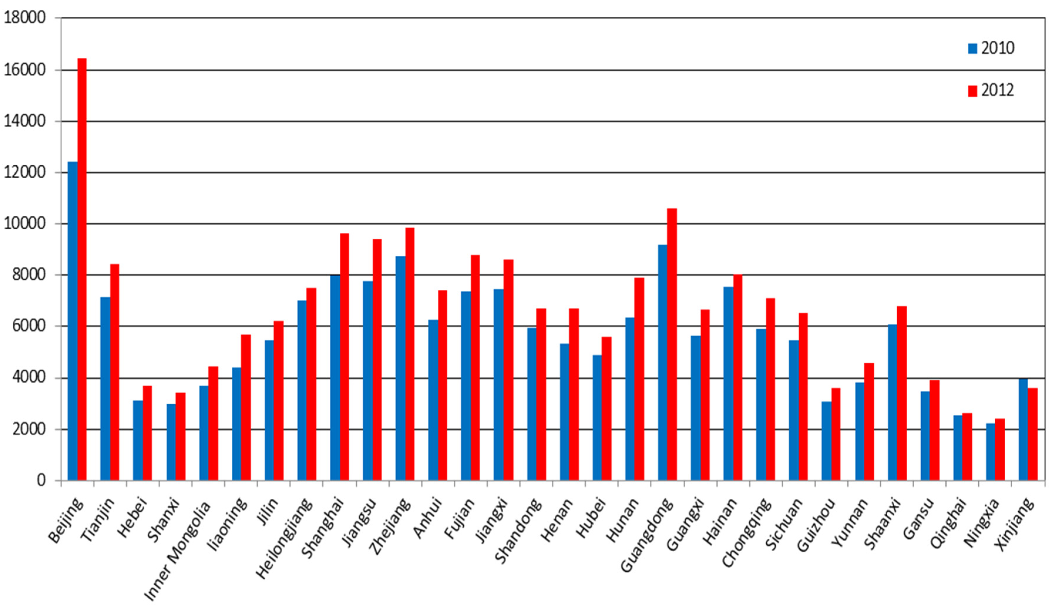
2010 is selected as the standard year, because in 2010, China’s “11th five-year” plan was completed and in that year, China’s energy economic indicators reached the scope stipulated in the “11th five-year” plan. This year is a representative of China’s implementation of a low carbon policy. 2012 is chosen as a comparison, because it is the latest year for which the statistical yearbook is available. Based preliminary on a histogram (Figure 1), this paper shows a comparison between 2010 and 2012 and reflects the situation of China’s provincial carbon productivity.

As shown in Figure 1, there exist obvious regional carbon productivity differences. For example, in 2012, the highest carbon productivity in Beijing is 6.85 times as much as that of the lowest carbon productivity in Ningxia. In addition, carbon productivity changes in various regions of China caused by unbalanced development will have a significant impact on China’s overall carbon productivity. Specifically, by raising the carbon productivity in Ningxia, Qinghai, Gansu and other areas that are lower than China’s overall carbon productivity, China’s carbon productivity will be improved significantly. At the same time, reducing CO₂ emissions will also significantly impact China’s carbon productivity, as this drives the different parts to adjust their respective economic structures and improve their energy productivities. In addition, due to the differences of regional economic development level and population size, we need to take the actual regional situation into account. Considering the different industry departments of the areas of China’s carbon productivity contribution value, further decomposition results need to be measured.

Figure 1. Actual productivity distribution of different provinces in 2010 and 2012.

Figure 1. Actual productivity distribution of different provinces in 2010 and 2012.

4. Result of Decomposition

Based on the decomposition model above, we can get carbon productivity contribution values from different parts and different industry structure of China. Specifically, according to the Equation (2), we order i = 30, and j = 6 to build a model which is suitable for China’s carbon productivity decomposition. After constructing a suitable decomposition model and putting the relevant data of China’s energy consumption into Equations (13)–(19), the contribution values of different regions’ influence factors and industrial structure can be calculated for the carbon productivity values. Parts of the calculation results are shown in Table 1 and Table 2.

Table 1. Different parts of Chinese influence factors’ contribution values to carbon productivity.

Province	Regional Actual Carbon Productivity	Carbon Intensity	Energy Structure	Energy Intensity	Economic Output	Population Size	The Reciprocal of per capita Carbon Emissions
Beijing	38.7113	0.5352	14.8008	−54.0408	36.2614	8.4354	−22.8392
Tianjin	24.0190	0.1184	−2.3577	−21.7699	34.0813	10.0142	−15.6998
Hebei	36.7925	0.8922	15.2227	−52.9057	72.9789	0.7384	−33.4899
Shanxi	19.8046	3.1717	−2.7664	−20.2074	34.7951	−0.0178	−15.1872
Inner Mongolia	34.1009	−4.9883	1.8702	−30.9818	51.0014	−0.5394	−19.5967
liaoning	50.1110	−11.0339	7.7866	−46.8610	78.4492	−1.9315	−30.8186
Jilin	21.2576	3.6588	−2.4127	−22.5011	40.4576	−1.1844	−14.6443
Heilongjiang	−24.0608	−6.0264	38.4214	−8.3114	41.1750	−1.5083	−17.1261
Shanghai	27.3271	−0.4392	20.1827	−47.0670	29.8562	5.1982	−26.7449
Jiangsu	64.0187	−1.4139	48.8484	−111.4335	153.0131	−2.3418	−68.0627
Zhejiang	32.9707	10.3460	5.0299	−48.3408	84.1153	−1.9069	−44.5718
Anhui	20.7573	0.3002	6.9183	−27.9630	59.2498	−0.9531	−20.9952
Fujian	34.5735	5.5594	0.7705	−40.8995	58.4847	0.9229	−24.5185
Jiangxi	19.6462	5.3802	−0.7658	−24.2569	42.1090	−0.1470	−15.9234
Shandong	63.4751	4.0882	−6.2499	−61.2759	129.0474	−0.2032	−63.6231
Henan	19.1873	4.7644	53.7608	−77.6998	80.7496	−3.3611	−37.5924
Hubei	31.0591	−5.8958	4.7373	−29.8930	75.8637	−0.3690	−27.1381
Hunan	37.1857	14.5392	5.3356	−57.0511	73.4291	0.0030	−27.1337
Guangdong	66.5238	5.9614	26.8279	−99.3070	128.0454	2.6229	−73.6763
Guangxi	20.7437	−2.7647	−0.9724	−17.0020	40.8434	0.7044	−16.0742
Hainan	1.9520	0.2098	−0.7570	−1.4037	9.1941	0.3046	−3.4953
Chongqing	19.6241	1.3569	4.2620	−25.2198	40.7408	1.2028	−13.6904
Sichuan	36.3830	−9.5866	3.8791	−30.6699	82.0001	−1.6633	−29.1622
Guizhou	18.9496	0.6623	−8.8900	−10.7185	27.7939	−0.6306	−8.0956
Yunnan	−37.8568	4.2566	13.5845	−25.0928	43.2598	0.2363	−14.5562
Shaanxi	23.0524	5.1698	−4.6688	−23.5466	52.9806	−0.8487	−17.4229
Gansu	8.2240	1.0808	−1.7204	−7.5804	18.5532	−0.2061	−6.9441
Qinghai	2.5526	−1.0097	−2.1945	0.6528	6.3858	0.1429	−2.3023
Ningxia	4.4994	1.0738	−2.3084	−3.2639	7.5425	0.2836	−2.8633
Xinjiang	2.4125	5.1877	−8.1343	1.4568	22.5180	0.8462	−8.6547

Table 1. Different parts of Chinese influence factors’ contribution values to carbon productivity.

Province	Regional Actual Carbon Productivity	Carbon Intensity	Energy Structure	Energy Intensity	Economic Output	Population Size	The Reciprocal of per capita Carbon Emissions
Beijing	38.7113	0.5352	14.8008	−54.0408	36.2614	8.4354	−22.8392
Tianjin	24.0190	0.1184	−2.3577	−21.7699	34.0813	10.0142	−15.6998
Hebei	36.7925	0.8922	15.2227	−52.9057	72.9789	0.7384	−33.4899
Shanxi	19.8046	3.1717	−2.7664	−20.2074	34.7951	−0.0178	−15.1872
Inner Mongolia	34.1009	−4.9883	1.8702	−30.9818	51.0014	−0.5394	−19.5967
liaoning	50.1110	−11.0339	7.7866	−46.8610	78.4492	−1.9315	−30.8186
Jilin	21.2576	3.6588	−2.4127	−22.5011	40.4576	−1.1844	−14.6443
Heilongjiang	−24.0608	−6.0264	38.4214	−8.3114	41.1750	−1.5083	−17.1261
Shanghai	27.3271	−0.4392	20.1827	−47.0670	29.8562	5.1982	−26.7449
Jiangsu	64.0187	−1.4139	48.8484	−111.4335	153.0131	−2.3418	−68.0627
Zhejiang	32.9707	10.3460	5.0299	−48.3408	84.1153	−1.9069	−44.5718
Anhui	20.7573	0.3002	6.9183	−27.9630	59.2498	−0.9531	−20.9952
Fujian	34.5735	5.5594	0.7705	−40.8995	58.4847	0.9229	−24.5185
Jiangxi	19.6462	5.3802	−0.7658	−24.2569	42.1090	−0.1470	−15.9234
Shandong	63.4751	4.0882	−6.2499	−61.2759	129.0474	−0.2032	−63.6231
Henan	19.1873	4.7644	53.7608	−77.6998	80.7496	−3.3611	−37.5924
Hubei	31.0591	−5.8958	4.7373	−29.8930	75.8637	−0.3690	−27.1381
Hunan	37.1857	14.5392	5.3356	−57.0511	73.4291	0.0030	−27.1337
Guangdong	66.5238	5.9614	26.8279	−99.3070	128.0454	2.6229	−73.6763
Guangxi	20.7437	−2.7647	−0.9724	−17.0020	40.8434	0.7044	−16.0742
Hainan	1.9520	0.2098	−0.7570	−1.4037	9.1941	0.3046	−3.4953
Chongqing	19.6241	1.3569	4.2620	−25.2198	40.7408	1.2028	−13.6904
Sichuan	36.3830	−9.5866	3.8791	−30.6699	82.0001	−1.6633	−29.1622
Guizhou	18.9496	0.6623	−8.8900	−10.7185	27.7939	−0.6306	−8.0956
Yunnan	−37.8568	4.2566	13.5845	−25.0928	43.2598	0.2363	−14.5562
Shaanxi	23.0524	5.1698	−4.6688	−23.5466	52.9806	−0.8487	−17.4229
Gansu	8.2240	1.0808	−1.7204	−7.5804	18.5532	−0.2061	−6.9441
Qinghai	2.5526	−1.0097	−2.1945	0.6528	6.3858	0.1429	−2.3023
Ningxia	4.4994	1.0738	−2.3084	−3.2639	7.5425	0.2836	−2.8633
Xinjiang	2.4125	5.1877	−8.1343	1.4568	22.5180	0.8462	−8.6547

Table 2. Different parts of Chinese industrial structure’s contribution values to carbon productivity.

Province	Primary Industry	Industry	Construction	Transport, Storage and Post	Wholesale, Retail Trade and Hotel, Restaurants	Others
Beijing	0.1069	1.8614	0.6630	0.1019	1.1787	17.9521
Tianjin	0.0757	13.0873	0.6279	0.2292	5.6853	8.7000
Hebei	3.2695	19.5715	2.1435	2.7184	4.4168	8.1094
Shanxi	0.8110	8.6498	0.6386	1.2333	2.7944	5.4655
InnerMongolia	2.4101	15.9273	2.5218	2.2451	3.2645	4.4974
liaoning	3.5728	19.1145	3.2535	2.8737	4.5110	12.3764
Jilin	2.5821	13.1527	1.6338	0.4441	1.9686	4.8503
Heilongjiang	−0.0195	−3.6900	−0.1947	−0.5970	4.0371	8.7771
Shanghai	−0.0195	−3.6900	−0.1947	−0.5970	4.0371	8.7771
Jiangsu	6.2768	23.8714	4.7296	4.0512	10.5031	33.1962
Zhejiang	1.4568	11.4752	1.3785	0.6743	8.7018	13.9557
Anhui	2.5426	22.1125	2.4726	0.6128	3.1116	6.4622
Fujian	2.6872	15.0188	4.3212	1.1914	2.5539	9.1204
Jiangxi	1.7670	11.2867	1.9399	1.4540	3.0695	6.5254
Shandong	2.4741	16.4163	2.8191	3.2787	23.0981	17.1724
Henan	0.8659	17.0872	2.4294	1.8856	7.2740	10.2667
Hubei	4.8321	24.6024	3.2427	0.9369	3.4779	11.2723
Hunan	4.2827	23.2160	2.2257	1.5615	3.2706	11.7513
Guangdong	2.9594	17.1325	1.5281	3.4719	13.4509	18.4553
Guangxi	3.1834	10.5224	2.6818	0.9457	3.8312	4.3138
Hainan	1.1596	0.9841	0.8481	0.2082	0.8230	1.9814
Chongqing	1.9001	9.1929	2.8521	0.8565	1.9704	11.5042
Sichuan	5.6203	24.7874	4.3869	0.6592	3.1419	12.5843
Guizhou	2.1379	5.8019	1.6273	1.6667	1.8604	5.9770
Yunnan	4.6430	5.8080	3.1069	0.3310	4.4052	−34.4626
Shaanxi	2.9096	19.5875	2.5733	0.9240	3.0388	5.6827
Gansu	1.1775	2.9468	1.1270	0.7242	1.4145	4.0170
Qinghai	0.2790	2.3352	0.5595	0.0279	0.2333	0.7927
Ningxia	0.2188	1.7439	0.8303	0.3719	0.3582	1.4405
Xinjiang	15.2862	4.6564	1.6698	1.2334	1.6880	−8.9016

Table 2. Different parts of Chinese industrial structure’s contribution values to carbon productivity.

Province	Primary Industry	Industry	Construction	Transport, Storage and Post	Wholesale, Retail Trade and Hotel, Restaurants	Others
Beijing	0.1069	1.8614	0.6630	0.1019	1.1787	17.9521
Tianjin	0.0757	13.0873	0.6279	0.2292	5.6853	8.7000
Hebei	3.2695	19.5715	2.1435	2.7184	4.4168	8.1094
Shanxi	0.8110	8.6498	0.6386	1.2333	2.7944	5.4655
InnerMongolia	2.4101	15.9273	2.5218	2.2451	3.2645	4.4974
liaoning	3.5728	19.1145	3.2535	2.8737	4.5110	12.3764
Jilin	2.5821	13.1527	1.6338	0.4441	1.9686	4.8503
Heilongjiang	−0.0195	−3.6900	−0.1947	−0.5970	4.0371	8.7771
Shanghai	−0.0195	−3.6900	−0.1947	−0.5970	4.0371	8.7771
Jiangsu	6.2768	23.8714	4.7296	4.0512	10.5031	33.1962
Zhejiang	1.4568	11.4752	1.3785	0.6743	8.7018	13.9557
Anhui	2.5426	22.1125	2.4726	0.6128	3.1116	6.4622
Fujian	2.6872	15.0188	4.3212	1.1914	2.5539	9.1204
Jiangxi	1.7670	11.2867	1.9399	1.4540	3.0695	6.5254
Shandong	2.4741	16.4163	2.8191	3.2787	23.0981	17.1724
Henan	0.8659	17.0872	2.4294	1.8856	7.2740	10.2667
Hubei	4.8321	24.6024	3.2427	0.9369	3.4779	11.2723
Hunan	4.2827	23.2160	2.2257	1.5615	3.2706	11.7513
Guangdong	2.9594	17.1325	1.5281	3.4719	13.4509	18.4553
Guangxi	3.1834	10.5224	2.6818	0.9457	3.8312	4.3138
Hainan	1.1596	0.9841	0.8481	0.2082	0.8230	1.9814
Chongqing	1.9001	9.1929	2.8521	0.8565	1.9704	11.5042
Sichuan	5.6203	24.7874	4.3869	0.6592	3.1419	12.5843
Guizhou	2.1379	5.8019	1.6273	1.6667	1.8604	5.9770
Yunnan	4.6430	5.8080	3.1069	0.3310	4.4052	−34.4626
Shaanxi	2.9096	19.5875	2.5733	0.9240	3.0388	5.6827
Gansu	1.1775	2.9468	1.1270	0.7242	1.4145	4.0170
Qinghai	0.2790	2.3352	0.5595	0.0279	0.2333	0.7927
Ningxia	0.2188	1.7439	0.8303	0.3719	0.3582	1.4405
Xinjiang	15.2862	4.6564	1.6698	1.2334	1.6880	−8.9016

According to the data in Table 1 and Table 2, this article will analyze the contribution values of China’s carbon productivity from the influencing factors, the provincial and the industrial structures.

5. Discussions

5.1. Overall Discussions

Table 1 reflects the contribution value of different influence factors in the regions on the carbon productivity. From Table 1, we can see roughly that in each region, the reciprocal of per capita carbon emissions to the carbon productivity contribution values are negative; to some extent, this illustrates that China’s population growth is slower than the increase of CO₂ emissions. According to the 2010 and 2012 China statistical yearbook, in 2010, China’s population was 1.33 billion, and in 2012, China’s population was 1.34 billion. The population rose 1.05% compared with 2010. China’s CO₂ emissions from energy consumption were 7.55 billion tons in 2010 and 8.56 billion tons in 2012. CO₂ emissions increased its year-on-year number by 13.38%. From the above data analysis, we can roughly speculate that attributing the rapid growth in China’s CO₂ emissions to China’s industrial structure, energy structure in different regions and even economic output is not reasonable. The true reason needs to be further studied.

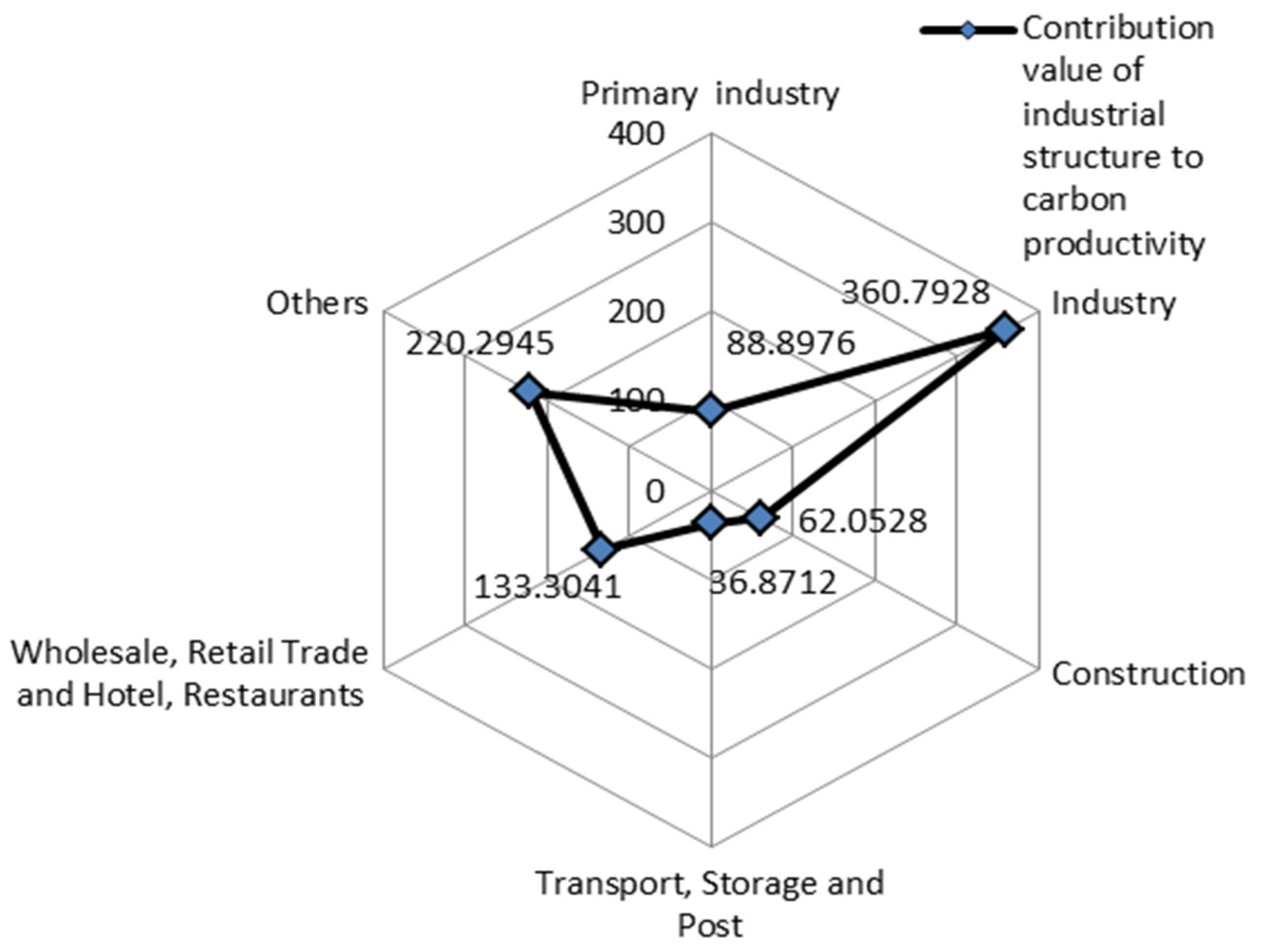
According to the six major industrial structures, the decomposed results of the contribution values in different industrial structures and influence factors of different provinces are summed. Then, the paper obtains the contribution values of different parts of Chinese industrial structure’s to carbon productivity. The specific decomposition results are shown in Table 2. Table 2 mainly reflects the carbon productivity contribution value of the industrial structures of different regions in China. From Table 2 we can see that Chinese industry’s contribution to the carbon productivity is greater than other industries. The specific reason will be analyzed in terms of industrial structure in this paper.

5.2. Discussions on the Dimension of Affecting Factors

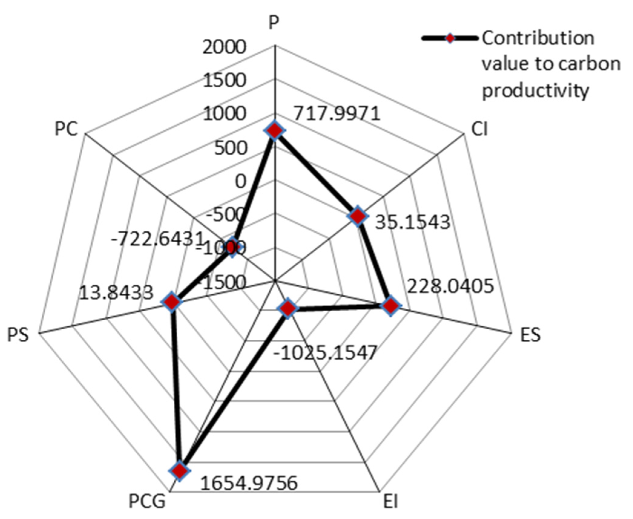
We can obtain the total contribution value of carbon productivity of different affecting factors through adding each province’s contribution value of carbon productivity by different affecting factors in Table 1. The result is shown in Figure 2.

Figure 2. Contribution value to carbon productivity.

Figure 2. Contribution value to carbon productivity.

As is shown in Figure 2, the output of GDP (PCG) has the highest contribution values. Followed by the actual carbon productivity of each province (P), energy structure (ES), carbon intensity (CI), population scale (PS), per capita carbon emission reciprocal (PC) and energy intensity (EI). The balance is 2680.13 between economic structure which contributes most values and energy intensity which made the lowest contribution values. Apart from PC and EI whose carbon productivity contribution values are negative, and other affecting factors are all positive. According to the above analysis, the main reason why PC has a negative contribution value of carbon productivity is that during 2010 to 2012, the increase of China’s CO₂ emissions was larger than the actual population growth. From the above analysis, and considering the reality that China has a big population base and at the same time, China is facing the reality of stepping into an aged society although the two-child policy has been relaxed, with all things considered, we can roughly speculate that in the near future, there is little possibility that China’s population will change a lot. Therefore, only by controlling the amount of CO₂ emissions can each province offset this factor’s negative effect on carbon productivity. Other affecting factors’ contributions to carbon productivity will be analyzed in the latter part of this paper.

5.2.1. Discussions of Each Province’s Actual Carbon Productivity

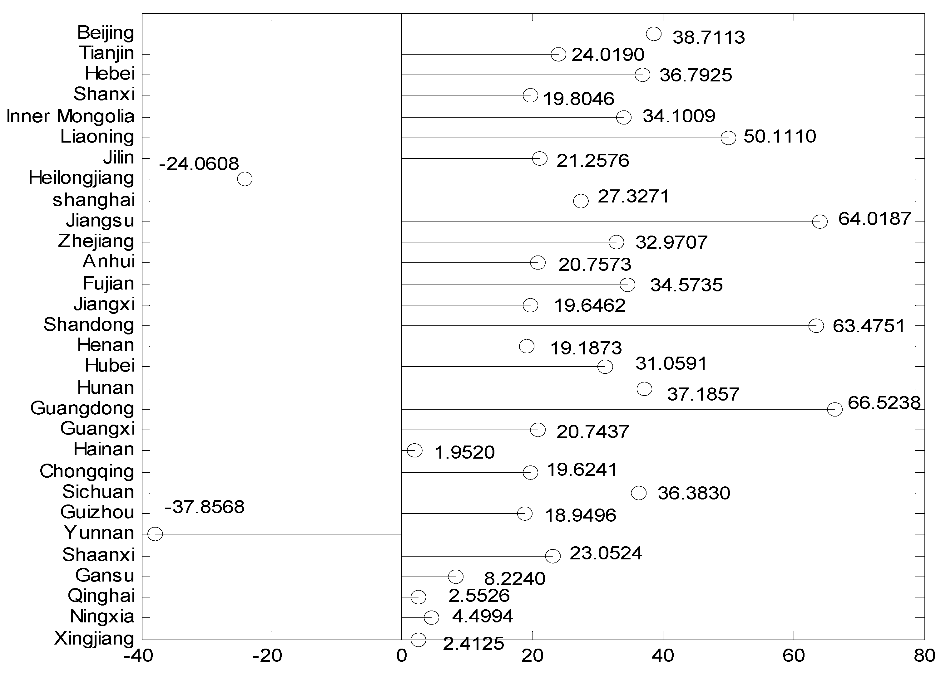
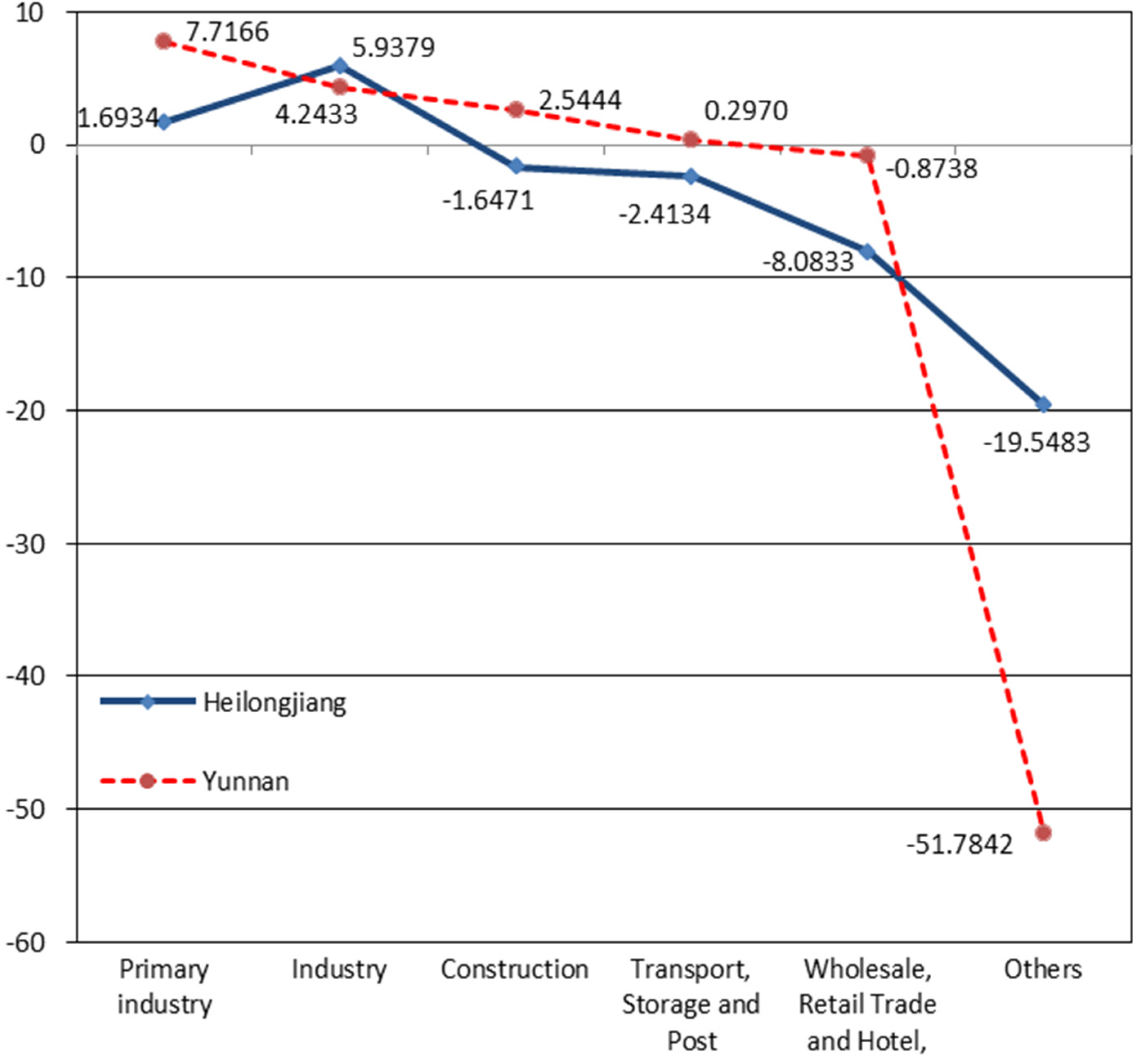
As is shown in Figure 3, only Heilongjiang and Yunnan have negative contribution to China’s carbon productivity. From Figure 4, we can see that in Yunnan, wholesale, retail trade and hotel, restaurants and others have negative contribution to China’s carbon productivity as affecting factors of actual regional carbon productivity. Apart from the primary industry and industry of Heilongjiang, other industries all have negative contributions to China’s carbon productivity in the affecting factors of actual regional carbon productivity. The reason is that Yunnan underwent a sustained severe drought in 2012 and continuous earthquakes occurred in the northeast. These disasters caused a great shock to Yunnan’s economy.

Figure 3. The contribution of provincial carbon productivity to China’s carbon productivity.

Figure 3. The contribution of provincial carbon productivity to China’s carbon productivity.

Figure 4. Yunnan and Heilongjiang provinces’ carbon productivity specific contribution value.

Figure 4. Yunnan and Heilongjiang provinces’ carbon productivity specific contribution value.

Besides, a sustained downturn in the real estate market of Yunnan made its real estate industry shrink substantially. Meanwhile, the downturn in the real estate market made real estate developers strictly curtail budgets for greening construction and consciously reduce their green investments, which also affected Yunnan’s landscaping industry. According to statistics, in 2012 Yunnan’s real estate, finance, tourism and other industries had a GDP contribution of 261,788 million yuan, while Yunnan’s related industries had a GDP contribution of 490,862 million yuan in 2010, which represents a decrease by 46.67%. The above industries’ amount of CO₂ was 605.50 thousand tons in 2012 while the amount of CO₂ was 365.34 thousand tons in 2010, an increase by 65.74%, which explains why Yunnan’s carbon productivity has a negative contribution to China’s carbon productivity. Heilongjiang is located in the northeast of China. Due to its failure to adjust its industrial development pattern in time, Heilongjiang is affected by China’s economic constraints. According to the statistics, construction enterprises that have a qualification of level three and above (general contracting and professional contracting enterprise excluding labor subcontracting enterprises) realized a profit of 5.63 billion yuan in 2012. The profit in 2010 was 5.68 billion yuan, or a decrease by 46.67% year-on-year. In the aspect of foreign economy, the total import and export value was 37.82 billion dollars in 2012, a 1.81% decrease compared to that in 2010. In the transportation aspect, the number of civil motor vehicles in Heilongjiang increased evidently. In 2012, civil vehicles reached to 2.69 million, while in 2010, the civil vehicles were 2.08 million, as increase by 29.33% year-on-year. The increase in the number of civil vehicles caused the increase in CO₂ emissions. This is the main reason why the carbon productivity in transportation and postal storage industry is negative in Heilongjiang. The sharp rise in the number of people in the tourist industry and the increased amount of coal used to provide heating causes that when other industry is increasing steadily, the CO₂ emissions are evidently increasing. According to the statistics, in 2012, the CO₂ emissions of other industries in Heilongjiang was 9.35 million tons, while the amount in 2010 was 3.88 million tons, an increase by 140.98% year-on-year. The sharp increase of CO₂ emissions is the main reason why other industries’ affecting factors of carbon productivity in Heilongjiang had a negative contribution value to China’s carbon productivity.

Apart from Yunnan Province and Heilongjiang Province, other provinces’ carbon productivity affecting factors have a positive contribution value to China’s carbon productivity. Some districts’ contribution values are relatively high, such as Liaoning, Jiangsu, Shandong and Guangdong. The CO₂ emissions in these provinces increased steadily by their improvement of technology. On the premise of this, these provinces make a great contribution to China’s carbon productivity by the sharp increase of GDP. Take Liaoning for example, in 2010, the GDP of Liaoning was 184.57 billion, the CO₂ emissions were 417.74 million tons. In 2012, the GDP was 248.46 billion, a 34.62% increase. The CO₂ emissions were 436.57 million tons, a 4.51% increase. Thus, technology improvement is the effective in the above region.

However, in some districts such as Hainan, Gansu, Qinghai, Ningxia and Xinjiang, the carbon productivity makes a small contribution to China’s carbon productivity. Because these districts are restricted by their location and historical development, their economy cannot develop rapidly in the short term. Therefore only by introducing new technology and reducing CO₂ emissions, can their corresponding contribution value be improved. The other districts such as Beijing, Tianjin, Hebei and other regions, have a moderate contribution value to China’s carbon productivity. The economy of these regions is developing rapidly, while, their CO₂ emissions are also increasing rapidly, so energy savings and emission reductions will be the top priority in these areas.

5.2.2. Discussions on Carbon Intensity

Figure 5 shows each province’s carbon emission intensity contribution value to China’s carbon productivity. Some provinces have a negative contribution value to carbon intensity, such as Inner Mongolia, Liaoning, Heilongjiang, Shanghai, Jiangsu, Hubei, Qinghai, Guangxi and Sichuan.

Figure 5. The contribution value of carbon intensity.

Figure 5. The contribution value of carbon intensity.

The reason is that these provinces have a low energy utilization ratio. Even though they have high energy consumption, they cannot be use the energy efficiently. Take Liaoning for example, in 2010, the energy consumption was 140.70 million tons of standard coal, and the CO₂ emissions were 417.73 million tons. In 2012, the energy consumption increased to 158.90 million tons of standard coal, as increase by 12.94% compared to that of 2010. The CO₂ emissions were 436.57 million tons, an increased by 4.51% compared to that of 2010. Evidently, the increase of energy consumption is the main reason that the carbon emission intensity is negative. However, the increase of energy consumption didn’t lead to an increase of GDP. For instance, the added value of GDP in Liaoning during 2010 to 2012 is 638.92 billion yuan, which is lower than that of 1105.49 billion yuan in Guangdong. However, the increase of energy consumption in Guangdong is just 6.14% during 2010 to 2012. Thus, we can roughly speculate that there is energy waste in the above provinces and the great amount of energy input has not achieved the expected economic output. Specific to the type of energy, if only the main fuels such as coal, coke, crude oil, gasoline, kerosene, diesel, fuel oil, liquefied petroleum gas are considered, the comparison of Liaoning and Guangdong is shown in Figure 6.

Figure 6. Energy consumption in Liaoning and Guangdong.

Figure 6. Energy consumption in Liaoning and Guangdong.

It can be seen that in the coke consumption, there are significant differences between the two provinces. The main reason is that in order to control the amount of CO₂ emissions, Guangdong has implemented measures to ban high pollution fuel combustion in the Pearl Delta except for Dongguan, and coke is a high-polluting fuel. In Liaoning, coke consumption mainly comes from industry. This indicates that energy waste in industry should be reduced. In other provinces which have positive carbon intensity like Beijing, Tianjin, Hebei, the value of the carbon emission intensity is relatively low. They mainly take measures to reduce energy waste and increase the energy utilization rate. In provinces that have a high contribution value, they also need to control their CO₂ emissions in a reasonable range so as to increase their influence to China’s carbon productivity while they are controlling their energy waste.

5.2.3. Discussions on Energy Structure

According to the China Energy Statistical Yearbook, in terms of specific energy structure, coal resources account have an absolute advantage in different regions. The central regions (Shanxi, Anhui, Jiangxi, Henan, Hubei, Hunan) have the highest percentage of coal resources. The perception is up to 96.6%. The proportions of other resources such as oil, natural gas and so on are at a relative disadvantage. Thus, this unreasonable energy structure will have great impact on carbon productivity. This affects the different industries in each province as well. In this section, the energy structure mainly refers to the energy consumption ratio in the different industries of the provinces. 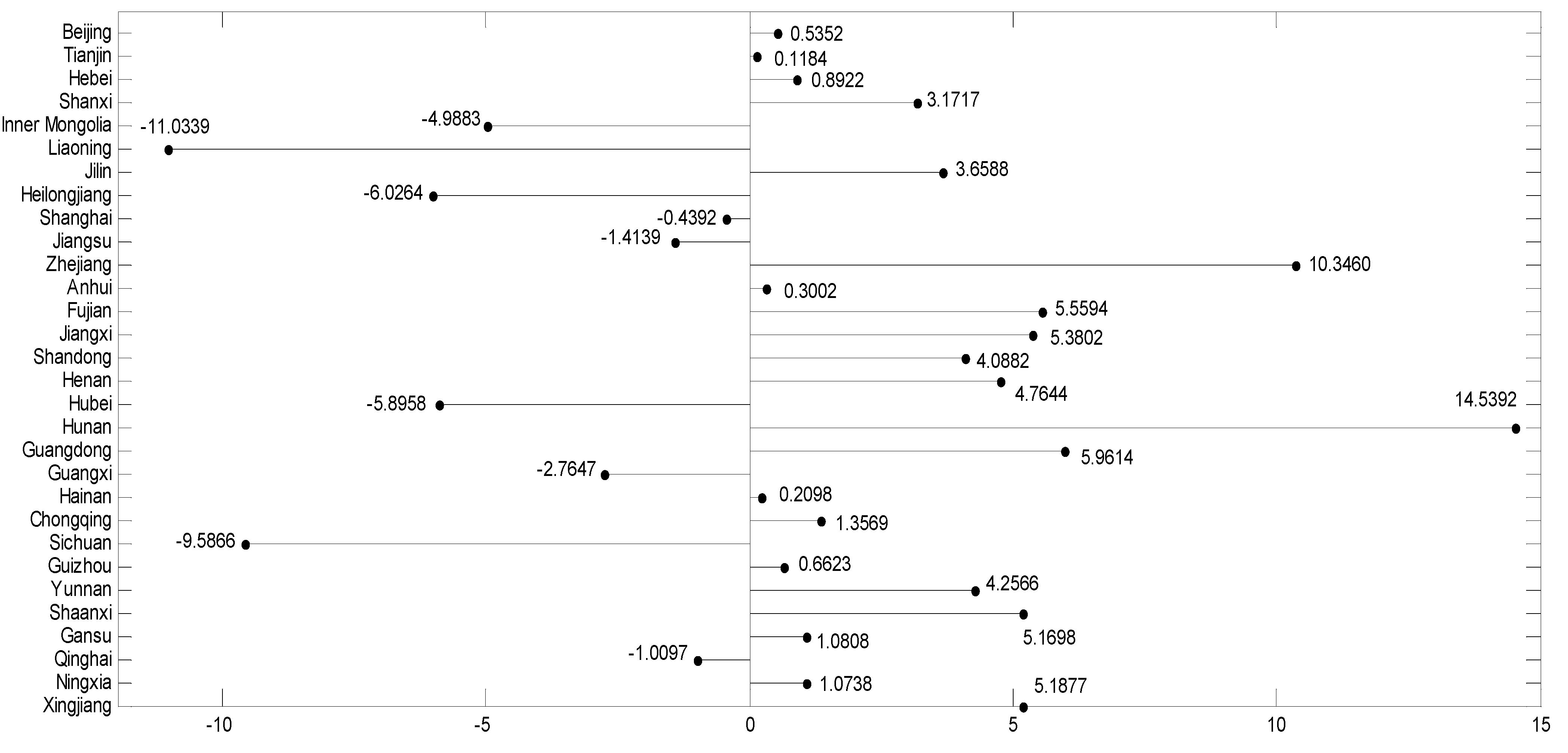Figure 7 shows the contribution value of the energy structure to China’s carbon productivity in different regions.

Figure 7. The contribution value of energy structure.

Figure 7. The contribution value of energy structure.

According to Equation (15), the affecting factor determined by measuring the proportion of energy consumption in the different industrial structures of different regions can be used as an effective method to measure whether the industrial structure is reasonable. In Figure 7, it is easy to find that the energy structures in Tianjin, Shanxi, Jilin, Shandong, Guangxi, Hainan, Guizhou, Shaanxi, Gansu, Qinghai, Ningxia and Xinjiang had a negative contribution value to China’s carbon productivity. As for a certain industry structure in a certain province, that has a negative contribution value, it means that the proportion of energy consumption is low in this certain industry structure and that this certain province does not pay much attention to this industry structure. As a result, an imbalance in the industry structure appears. Take Shanxi for example, in the aspect of energy structure, the contribution value of primary industry, industry, construction, transport, storage and post, wholesale, retail trade and hotel, restaurants and others are −0.2725, 0.4794, −0.42525, −0.2337, 0.3632 and −2.6775. As China’s coal heartland, Shanxi concentrates on the production and sale of coal, thus Shanxi will focus on industry and the wholesale and retail industry and it does not pay enough attention to other industries. According to the data in the Figure 7, the lower the contribution value of the energy structure is, the more its structure is. Take Henan which makes the highest contribution value for example, the contribution value is positive in all industries except for industry. That’s because Henan is not a traditional province featuring a strong industry sector. The contribution values of other industries are 9.5321, 4.8927, 4.5341, 14.65887 and 30.1362, leading the other provinces. Provinces which make a low contribution to energy structure should focus on how to adjust their industrial structure.

5.2.4. Discussions on Energy Intensity

Energy intensity mainly reflects the energy consumption per GDP output in a certain industry of a certain province. As shown in Table 1, apart from Qinghai and Xinjiang, the other provinces’ energy intensities all have a negative carbon productivity value. Although the contribution value of energy intensity in Qinghai and Xinjiang is positive, the contribution value is very low. The reason is that although technical progress has a great positive effect, these provinces do not put much emphasis on adjusting their industrial structure. This leads to a negative value of energy intensity. Since the contribution value of energy intensity to CO₂ varies among all the provinces, the contribution to carbon productivity can be improved by reducing some sectors’ energy intensity. By comparing data for the different provinces, we can conclude that energy intensity in industry is a main cause of the decrease of China’s carbon productivity. Therefore, in order to improve the contribution value of energy intensity to China’s carbon productivity, the authorities should reduce a sector’s energy intensity by improving the conversion and utilization efficiency in industry.

5.2.5. Analysis on Economic Output

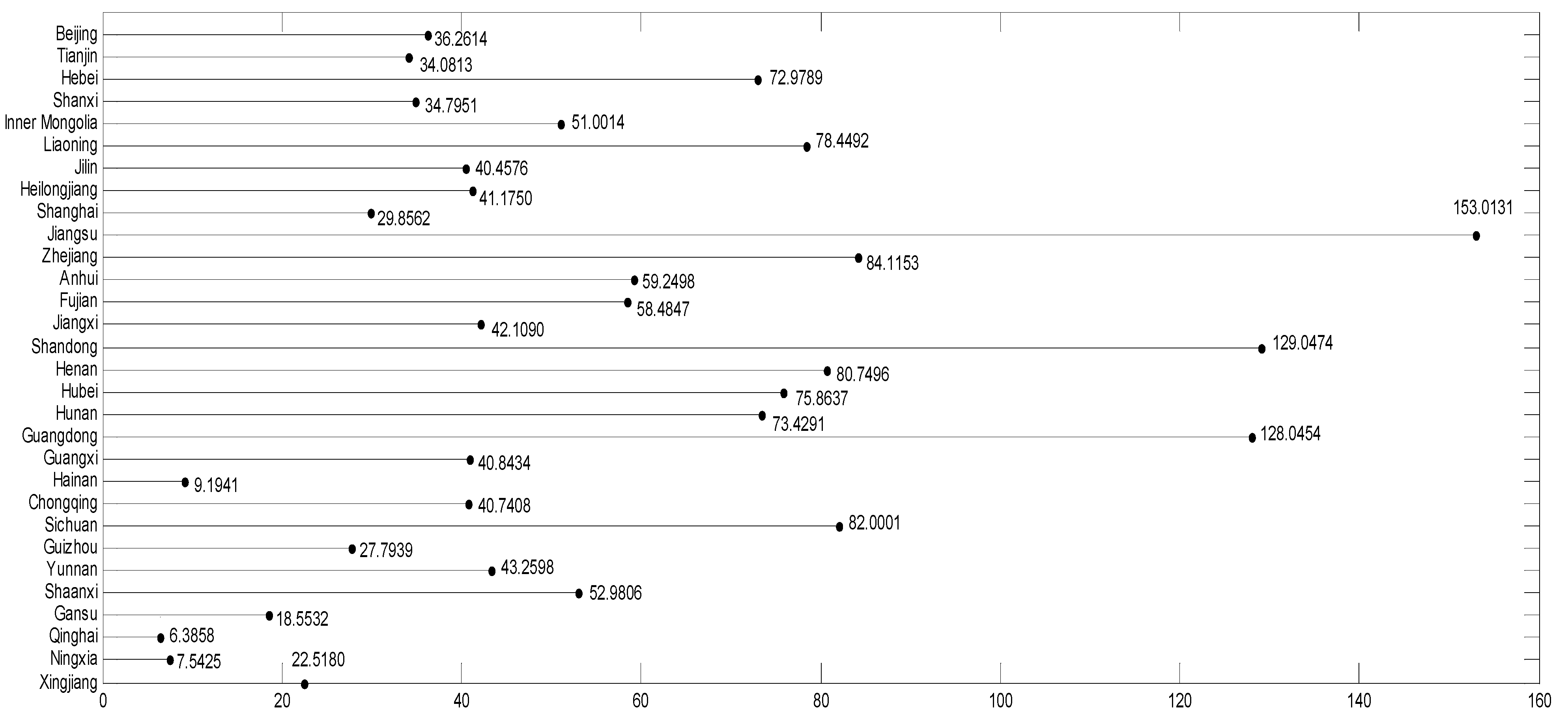
As is shown in Figure 8, economic output in all provinces has a positive contribution value to China’s carbon productivity.

Figure 8. The contribution value of economic output.

Figure 8. The contribution value of economic output.

However, the difference between Jiangsu, which has the highest contribution value of 153.0131, and Qinghai, which has the lowest contribution value of 6.3858, is 146.6273. As is proposed in the above, China’s population in the next period will not fluctuate widely, nor is that of the provinces, therefore, each province’s population and the speed of economic development will be the main factors affecting the contribution value of this factor to carbon productivity. While maintaining the economic development level of the provinces whose economic output contributes greater value to carbon productivity, by stabilizing population growth and earnestly implementing the national industrial structure adjustment implementation of this strategy, it may stimulate the economic structure of China’s relatively low carbon productivity to improve the regional influence.

5.2.6. Discussions on Population Scale

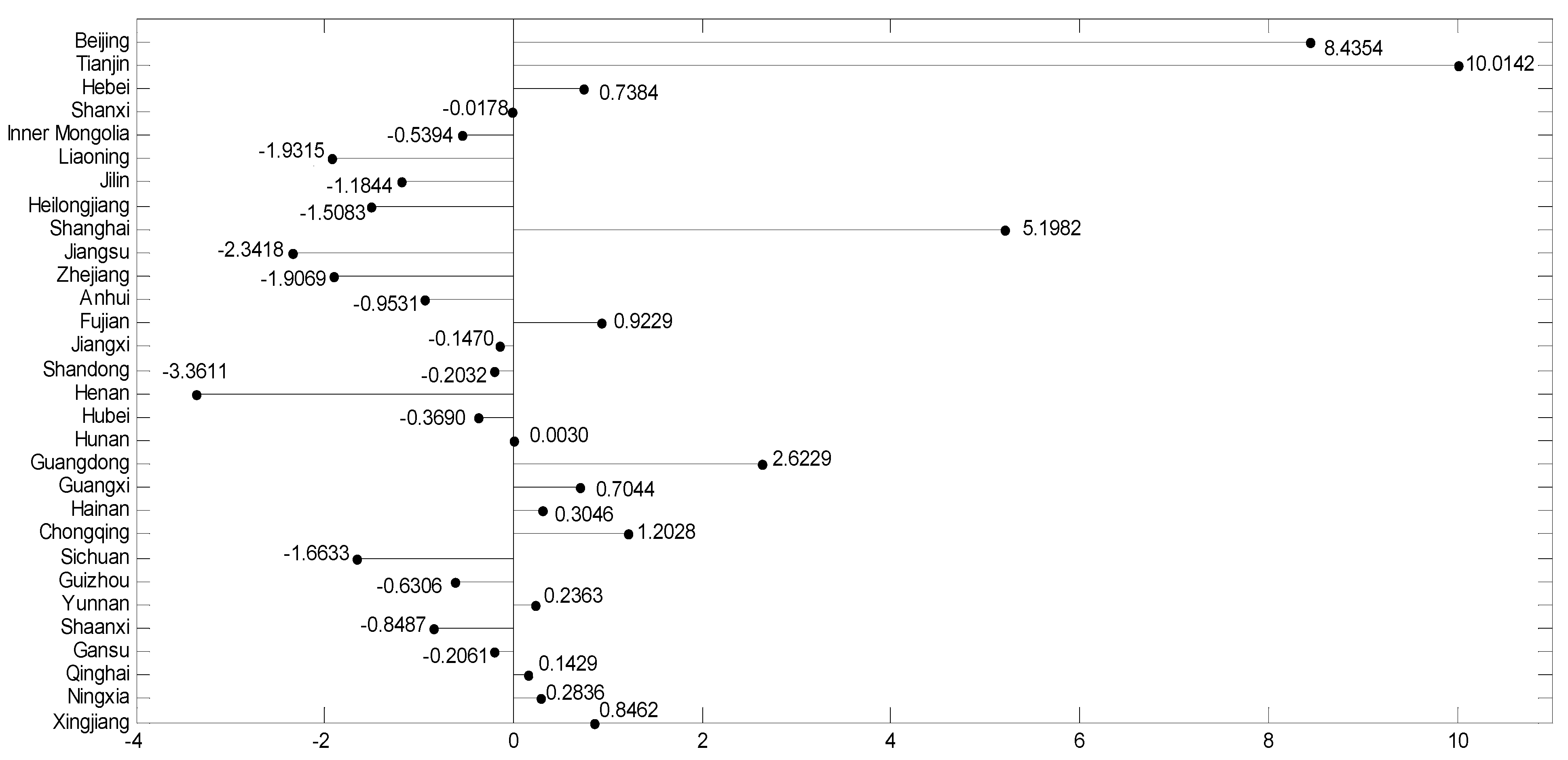
Generally speaking, as shown in Figure 2, the population scale has a positive contribution value to China’s carbon productivity. From Figure 9, apart from Tianjin (10.0142), Beijing (8.4354), shanghai (5.1982) and Guangdong (2.6229), other provinces’ contribution values are lower than 2. This indicates that apart from the above regions, the speed of population growth in other provinces is similar to that of China as a whole. As the main provinces experiencing net immigration, the speed of population growth in the above provinces is faster than that of the rest of China. This leads to a higher contribution value by the population scale in the above provinces than that of other provinces.

Figure 9. The contribution value of population scale.

Figure 9. The contribution value of population scale.

5.3. Discussions on Regional Dimension

Through the above factor analysis, the main factors driving the differences between the various regions of China’s carbon productivity contribution differences are economic output (PCG), carbon productivity (P), and energy structure (ES). Economic output is a scale effect influencing China’s carbon productivity through per capita GDP. Each province’s carbon productivity is the technical effect influencing the carbon productivity of China through the different levels of technological development in different regions. Energy structure is affected by the carbon productivity of various energy consumption sectors of different provinces, the so-called structural effects. This is similar to the policy “considering local realities, we should rely on technological progress and industrial structure to adjust and promote regional development”. In this regard, this paper can study a classification by considering these three factors from different provinces.

In order to reflect different regions of the economic output affecting China’s overall carbon productivity growth value, we define $RPC{G}_i$:

$$RPC{G}_i=\frac{PC{G}_i}{P_t-P_o}$$

(20)

wherein $P_t$ represents the carbon productivity of the comparison period, $P_o$ represents the carbon productivity of the base period. We define the $R{P}_i$ and $RE{S}_i$ by similar approaches. After measuring, in 2012, China’s carbon productivity was 6728.07 yuan/ton, and in 2010, China’s carbon productivity was 5784.97 yuan/ton. Through calculation, the values for the contributions of the different Chinese provinces of the above three kinds of influencing factors to China’s overall carbon productivity growth are shown in Table 3.

Table 3. Different parts of China’s three kinds of influencing factors of contribution rate.

Province	RPCGi	RPi	RESi	Province	RPCGi	RPi	RESi
Beijing	3.84%	4.10%	1.57%	Henan	8.56%	2.03%	5.70%
Tianjin	3.61%	2.55%	−0.25%	Hubei	8.04%	3.29%	0.50%
Hebei	7.74%	3.90%	1.61%	Hunan	7.79%	3.94%	0.57%
Shanxi	3.69%	2.10%	−0.29%	Guangdong	13.58%	7.05%	2.84%
Inner Mongolia	5.54%	3.62%	0.20%	Guangxi	4.33%	2.20%	−0.10%
Liaoning	8.32%	5.31%	0.83%	Hainan	0.97%	0.21%	−0.08%
Jilin	4.29%	2.25%	−0.26%	Chongqing	4.32%	2.08%	0.45%
Heilongjiang	4.37%	−2.55%	4.07%	Sichuan	8.69%	3.86%	0.41%
Shanghai	3.17%	2.90%	2.14%	Guizhou	2.95%	2.01%	−0.94%
Jiangsu	16.22%	6.79%	5.18%	Yunnan	4.59%	−4.01%	1.44%
Zhejiang	8.92%	3.50%	0.53%	Shaanxi	5.62%	2.44%	−0.50%
Anhui	6.28%	2.20%	0.73%	Gansu	1.97%	0.87%	−0.81%
Fujian	6.20%	3.67%	0.08%	Qinghai	0.68%	0.27%	−0.23%
Jiangxi	4.46%	2.08%	−0.08%	Ningxia	0.80%	0.48%	−0.24%
Shandong	13.68%	6.73%	−0.66%	Xinjiang	2.39%	0.26%	−0.86%

Table 3. Different parts of China’s three kinds of influencing factors of contribution rate.

Province	RPCGi	RPi	RESi	Province	RPCGi	RPi	RESi
Beijing	3.84%	4.10%	1.57%	Henan	8.56%	2.03%	5.70%
Tianjin	3.61%	2.55%	−0.25%	Hubei	8.04%	3.29%	0.50%
Hebei	7.74%	3.90%	1.61%	Hunan	7.79%	3.94%	0.57%
Shanxi	3.69%	2.10%	−0.29%	Guangdong	13.58%	7.05%	2.84%
Inner Mongolia	5.54%	3.62%	0.20%	Guangxi	4.33%	2.20%	−0.10%
Liaoning	8.32%	5.31%	0.83%	Hainan	0.97%	0.21%	−0.08%
Jilin	4.29%	2.25%	−0.26%	Chongqing	4.32%	2.08%	0.45%
Heilongjiang	4.37%	−2.55%	4.07%	Sichuan	8.69%	3.86%	0.41%
Shanghai	3.17%	2.90%	2.14%	Guizhou	2.95%	2.01%	−0.94%
Jiangsu	16.22%	6.79%	5.18%	Yunnan	4.59%	−4.01%	1.44%
Zhejiang	8.92%	3.50%	0.53%	Shaanxi	5.62%	2.44%	−0.50%
Anhui	6.28%	2.20%	0.73%	Gansu	1.97%	0.87%	−0.81%
Fujian	6.20%	3.67%	0.08%	Qinghai	0.68%	0.27%	−0.23%
Jiangxi	4.46%	2.08%	−0.08%	Ningxia	0.80%	0.48%	−0.24%
Shandong	13.68%	6.73%	−0.66%	Xinjiang	2.39%	0.26%	−0.86%

In order to further study the influence caused by the above three factors of Chinese provinces, the different influencing factors in Table 4 should be classified by high and low contribution values. After calculation, the average values of RPCG, RP, RES are 5.85%, 2.54%, 0.81%. According to the above three factors, China’s provinces are divided into eight categories, with the results shown in Table 4.

Table 4. Different areas of China’s classification criteria and classification results.

Series	Classification Standard	Classification Results
1	$RPCG>5.85\%,RP>2.54\%$	Hebei Liaoning Jiangsu
	$RES>0.81\%$	Guangdong
2	$RPCG<5.85\%,RP>2.54\%$	Beijing Shanghai
	$RES>0.81\%$
3	$RPCG>5.85\%,RP<2.54\%$	Henan Heilongjiang
	$RES>0.81\%$
4	$RPCG>5.85\%,RP>2.54\%$	Zhejiang Fujian Shandong
	$RES<0.81\%$	Hubei Hunan Sichuan
5	$RPCG<5.85\%,RP<2.54\%$	Yunnan
	$RES>0.81\%$
6	$RPCG<5.85\%,RP>2.54\%$	Inner Mongolia Tianjin
	$RES<0.81\%$
7	$RPCG>5.85\%,RP<2.54\%$	Anhui
	$RES<0.81\%$
8	$RPCG<5.85\%,RP<2.54\%$	Shanxi Jilin Jiangxi Guangxi Hainan Chongqing
	$RES<0.81\%$	Guizhou Shaanxi Gansu Qinghai Ningxia Xinjiang

Table 4. Different areas of China’s classification criteria and classification results.

Series	Classification Standard	Classification Results
1	$RPCG>5.85\%,RP>2.54\%$	Hebei Liaoning Jiangsu
	$RES>0.81\%$	Guangdong
2	$RPCG<5.85\%,RP>2.54\%$	Beijing Shanghai
	$RES>0.81\%$
3	$RPCG>5.85\%,RP<2.54\%$	Henan Heilongjiang
	$RES>0.81\%$
4	$RPCG>5.85\%,RP>2.54\%$	Zhejiang Fujian Shandong
	$RES<0.81\%$	Hubei Hunan Sichuan
5	$RPCG<5.85\%,RP<2.54\%$	Yunnan
	$RES>0.81\%$
6	$RPCG<5.85\%,RP>2.54\%$	Inner Mongolia Tianjin
	$RES<0.81\%$
7	$RPCG>5.85\%,RP<2.54\%$	Anhui
	$RES<0.81\%$
8	$RPCG<5.85\%,RP<2.54\%$	Shanxi Jilin Jiangxi Guangxi Hainan Chongqing
	$RES<0.81\%$	Guizhou Shaanxi Gansu Qinghai Ningxia Xinjiang

Traditionally, when enacting differential economic development policies in China, the government often considers two types of policies: one is based on the geographical location and the other depends on the level of economic development, but when considering the different sections of the carbon productivity distribution, Table 4 shows a different revelation:

(1)

Distribution patterns of different regions have nothing to do with the Chinese traditional sense of regional economic development.

In accordance with the relevant documents, China’s economic development area is divided into the Eastern, Central, Western regions and Northeast China. Taking the Eastern region for example, the provinces (municipalities) which belong to the Eastern region are as follows: Beijing, Tianjin, Shanghai, Hebei, Jiangsu, Zhejiang, Shandong, Fujian, Guangdong and Hainan. However, considering the region’s contribution to China’s carbon productivity, in the same area, Hebei, Jiangsu and Guangdong are in category 1; Beijing and Shanghai in category 2; Zhejiang, Shandong, Fujian in category 4; Tianjin in category 6; Hainan in category 8. So when we focus our research on China’s carbon productivity contribution value, the areas cannot be simply divided into four regions. On the contrary, we need specific analysis based on the local situations.

(2)

The distribution patterns of different provinces are partly associated with the region’s economic development level.

According to the statistics, in 2012, the top five provinces in China’s per capita GDP were Tianjin belonging to category 6; Beijing, Shanghai, belonging to category 2; Jiangsu belonging to category 1; and Zhejiang belonging to category 4. For the most underdeveloped five areas of Guizhou, Gansu, Yunnan, Guangxi, Jiangxi, in addition to Yunnan, the rest of the four areas are in class 8. For underdeveloped areas, in addition to Yunnan, the other four provinces can roughly use the same model to improve the region’s contribution values to the carbon productivity; for the developed areas, we need to take the actual situation of the region into consideration to determine in which category they are, and then determine its carbon productivity development pattern.

(3)

Considering regional protectionism, the actual regional situation needs to be considered at the same time.

From the above analysis, the energy structure impacts carbon productivity through various aspects of energy consumption in different provinces in China. By calculation, China’s carbon productivity contribution value in various areas is only 0.81%. Given that China is now actively promoting industrial structure adjustment, the reality can be concluded that the local government may impose local protectionism and hinder the implementation of this policy. As the consumption of fossil energy of a province can promote its own GDP and the GDP can be used as a core indicator for the performance of local governments, it is not hard to understand why local governments do not want to control the fossil energy consumption and emissions for their own interests. However, a question may be easily overlooked when talking about regional protectionism. That is, for the different population sizes and economic outputs of the provinces, what are the means that break the consistent regional protectionism? Considering the situation in various areas of inconsistencies, local protectionism cannot be treated the same. On the contrary, different measures should be taken on the basis of classification. As shown in Table 4, RES < 0.81% is 21 in total. It is enough to illustrate the severity of the local protectionism policy in China, but for RES > 5.85% provinces such as Zhejiang, Shandong, Fujian, governments take measures to limit local protectionism according to the obvious differences between RES < 5.85% provinces, because these measures to control CO₂ emissions will inevitably impact on regional GDP per capita, thereby reducing the overall scale of China’s carbon productivity contribution degree. When making policies for different areas, the government needs to have clear criteria to distinguish them.

5.4. Discussions on Industrial Sector Dimension

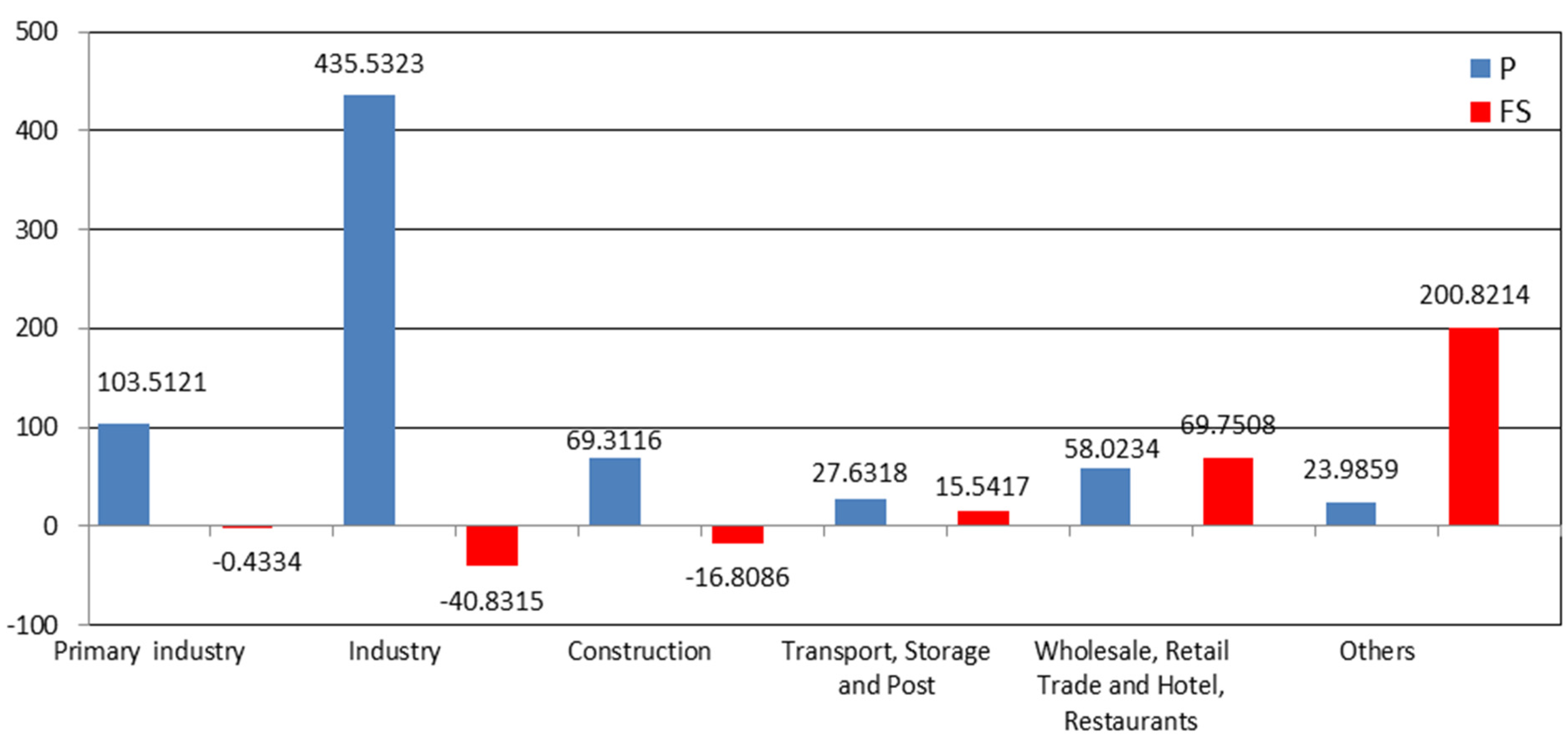
As shown in Figure 10, the industry’s contribution to China’s carbon productivity is more than that of other industrial structures, followed by “others”, wholesale retail trade and hotel, restaurants, primary industry, construction, and transport, storage, and postal activities. Due to the analysis by departments, this doesn’t involve the population, so we don’t need to think about economies of scale. Then, according to the analysis on the dimension of influencing factors, it is obvious that the economic output made the largest contributions to China’s carbon productivity, followed by regional carbon productivity and energy structure. Here, if applied to the industrial sector, carbon productivity and energy structure of industrial sectors should be considered. Sector carbon productivity can reflect different sectors due to the reasons of the progress of technology of carbon productivity contribution value; Energy structure can reflect contribution value to China’s carbon productivity of different industrial sectors due to industrial structure adjustment. The specific contribution value data as shown in Figure 11.

Figure 10. Contribution of industrial structure to the carbon productivity.

Figure 10. Contribution of industrial structure to the carbon productivity.

As mentioned above, the industry’s contribution to China’s carbon productivity is more than that of any other industrial structure. The reason may be that the industrial sector mainly relies on technological progress to improve its economic benefit, so the carbon productivity is improved; however, from 2010 to 2012, the proportion of China’s industrial sector CO₂ emissions becomes small, varying from 80.04% to 79.35%. This is the main reason that the energy structure contribution is very small, and even negative.

From Figure 11, we can see that the energy structure contribution values of first industry, industry, and construction are negative. Except for the above three groups, other groups’ energy structure contribution values are positive. Obviously, this is not reasonable. This also reflects that China’s industrial structure is not reasonable. From the point of view of promoting the development of China’s economy, by adjusting the industrial structure of China, thus adjusting the energy contribution value which are lower than the average level of the industry, the carbon productivity contribution value in China will increase to a certain extent. Taking the industrial sector as an example, on the basis of the control of new capacity, phasing out backward production capacity may effectively improve the contribution value of energy structure to China’s carbon productivity.

Figure 11. The contribution value in industry groups of two kinds of factors.

Figure 11. The contribution value in industry groups of two kinds of factors.

6. Conclusions

The changes in carbon productivity have always been considered as an important indicator to measure a country’s contribution in dealing with global climate change. In this paper, by using an LMDI decomposition model, a quantitative decomposition of the carbon productivity is performed. By considering the different influencing factors affecting carbon productivity, the change of carbon productivity is quantitatively decomposed into the provincial carbon productivity, carbon intensity, energy structure, energy intensity, economic output, population size and the reciprocal of per capita carbon emissions. On the basis of the results of the decomposition, from the three dimensions of the influencing factors, the regional and industrial sectors, this paper studied the contribution values of carbon productivity, aiming to find out the driving factors of carbon productivity growth.

Based on the above analysis, in order to better implement a low carbon policy in China, so as to control CO₂ emissions, and improve the efficiency of carbon productivity, the provinces of China should consider the following aspects:

(1)

Considering the huge contribution to carbon productivity from industry, government should take a series of actions to encourage key energy-consuming industrial enterprises to improve their levels of energy efficiency.

These actions mainly include setting specific energy saving targets, improving the enterprise energy management systems, formulating and reviewing energy efficiency improvements, energy saving target monitoring and supervision, and various assessments of rewards and punishments. The well-established government-enterprise cooperation platform also supports many other energy-saving actions, such as promoting the application of a particular process or equipment energy consumption standards, implementing regulations on eliminating backward production capacity, the government’s energy-saving special investment subsidies that can be requested and awarded and so on.

(2)

Adjust the industrial structure optimization.

Through the above analysis, a common unfavorable situation is that Chinese industrial structure adjustment is not satisfactory. Given the situation that our country has entered the intermediate industrialization stage where heavy industry predominates, heavy industry’s contribution to the economic growth is larger compared with other industries. The key point of economic restructuring and industrial upgrading is the transformation of economic growth modes, from a traditional extensive economic growth mode to an intensive economic growth pattern. In the long run, the use of technology to promote optimization and upgrading of industrial structure is the main driving force of the economic structure adjustment. Meanwhile, speeding up the transformation and upgrading of the traditional manufacturing and traditional services, developing modern manufacturing and modern service industries are also indispensable. At the same time, energy conservation and emissions reduction is an effective means to adjust the economic structure and transform the mode of growth. Through energy conservation and building innovation capacity, it is better to develop high-tech industries and modern service industries, to limit the development of high energy-consuming industries and to eliminate backward production capacity so as to improve the level of traditional industries, and constantly promote the optimization and upgrading of industrial structures.

(3)

Implement measures to reduce emissions by regions.

Based on the above analysis, considering the contributions to the carbon productivity value in various regions, the distribution patterns of different regions have nothing to do with the Chinese traditional sense of the regional economic development patterns. When implementing measures concerning energy conservation and emissions reduction, the diversity of the local actual situation also needs to be considered to determine the regional energy conservation and emissions reduction targets. When China sets energy conservation and emissions reduction targets, it is necessary to do more field investigations, combined with comprehensive appraisals of the economic development level and regional problems of energy conservation and emissions reduction and emissions reduction potential. Meanwhile, for economically less-developed areas, the central government should increase financial support, improving the financial transfer payment system between horizontal sectors and putting guarantee funds in place. At the same time, the central government should ensure economic developed areas offer counterpart support to underdeveloped areas.

(4)

To break the regional protectionism.

A province where fossil energy is consumed can promote its own GDP growth, but it would create CO₂ emissions around the area, and even impact global climate change. Due to the fact GDP growth is related to the interests of local governments, and any adjustment of the industrial structure tends to have a significant side effect on GDP, local governments are reluctant to see this happen. If China wants to improve the carbon productivity, it is necessary to break the regional protectionism.