Performance Evaluation of Air-Based Heat Rejection Systems

Abstract

On the basis of the Number of Transfer Units (NTU) method a functional relation between electric power for fans/pumps and effectiveness in dry coolers and wet cooling towers is developed. Based on this relation, a graphical presentation method of monitoring and simulation data of heat rejection units is introduced. The functional relation allows evaluating the thermodynamic performance of differently sized heat rejection units and comparing performance among them. The method is used to evaluate monitoring data of dry coolers of different solar cooling field projects. The novelty of this approach is that performance rating is not limited by a design point or standardized operating conditions of the heat exchanger, but is realizable under flexible conditions.

1. Introduction

Heat rejection is essential for a variety of processes in industrial, commercial and residential applications. In the latter two cases it is mostly used in air conditioning, cooling and refrigeration applications. The use of these technologies is ever increasing, e.g., according to [1] the market growth across the world only for air conditioning systems is expected to be above 5% for the next 3 years. One consequence of this enormous growth is an increase in electricity consumption for cooling processes. Considering the actual climate discussion and motivated by rising electricity prices around the globe, efforts are made by many stakeholders to increase the efficiency of the involved components (among which heat rejection plays a key role).

Waste heat from cold processes can be dissipated to different media such as water, soil and air. Therefore technologies used for heat rejection include night radiative cooling [2], sea-, lake- or groundwater cooling, including buried irrigation tanks [3] or swimming pools [4]. Yet the most commonly used heat sink is ambient air, as the above named options are rarely available or costly to exploit. As a result this study will concentrate on the air based technologies (e.g., dry coolers, wet cooling towers).

A first step towards the increase of efficiency is the determination of actual performance of heat rejection unit. Therefore standards for the determination of performance of heat rejection units exist. Some of the standards and performance evaluation methods will be presented below, to show the limitations of evaluation and the necessity of a more flexible method.

For dry coolers the European norm [5] defines one reference operating point at which the nominal capacity is determined (fixed temperatures for the air (25 °C) and water side (40 °C) and a fixed atmospheric pressure of 1013 hPa). Instructions on measurements and correction factors for differing conditions are given. The European Committee of Air Handling and Refrigeration Manufacturers (Eurovent) published a guideline for rating dry coolers [6]. Based on the standard defined in [5], the electric power for the fan/fans is measured. If the standard conditions are not fulfilled, instructions to correct the measurements are given. An energy ratio $R$, defined as nominal cooling capacity divided by the total certified power input of the fan motors at the standard rating conditions, is then calculated. Based on this value, a rating of dry coolers in an energy class (A++ for $R \ge 240$ to E with $R >30$) can be performed. However the rating is limited to the standard operating point. Performance under varying conditions is left open. In [7] the German standard, according to which the energy consumption of buildings shall be determined, single average seasonal values for the electricity consumption of heat rejection equipment (including fans and pumps) are specified:

• dry heat rejection systems: 0.045 ${\text{kW}}_{\text{el}}/{\text{kW}}_{\text{th}}$;
• open wet cooling towers with axial fan: 0.018 ${\text{kW}}_{\text{el}}/{\text{kW}}_{\text{th}}$;
• closed wet cooling towers with axial fan: 0.033 ${\text{kW}}_{\text{el}}/{\text{kW}}_{\text{th}}$.

The performance testing of series wet cooling towers must be carried out according to European Standard (EN) 13741 [8]. In this standard the procedure to verify the performance specified by the manufacturer is described. Yet the boundary conditions under which this is done are left up to the manufacturer. Therefore no comparability among products is facilitated, no labelling is possible. In [9] performance curves and tower characteristic maps for wet cooling towers are presented. The temperature range on the cold water side can be read off for different design flow rates, wet-bulb temperatures and cold water temperatures. Yet the method does not facilitate an easy comparison of different products nor does it allow the rating of different products. Also, a depiction of monitoring data in a similar way is precluded, if the available data is insufficient.

Apparently there is no description of performance or a definition of a satisfying coefficient of performance which allows the comparison of different Heat Rejection Units (HRUs). Especially as in practice HRUs rarely operate under the reference conditions defined in the standards, the question of their actual performance is open. This is even more so, as more and more frequently efforts are made to control both the air and the water volume flow according to the actual ambient conditions and load variations in order to minimize the auxiliary electricity consumption of such systems. One possibility to handle these flexible conditions is an annual and site specific simulation of the whole system including a suitable control strategy for the HRU. However, these simulations are time consuming and very specific and therefore not appropriate for evaluation of different HRUs. Consequently a method to evaluate HRUs not only in their design point or as one component in a whole system, but as an independent unit has to be elaborated.

In this paper we will develop a presentation method for the performance characterization of dry coolers by means of monitoring and simulation data at flexible operating conditions. We then extend this method to compare HRUs of different size and we illustrate the applicability of this method for monitoring and simulation data of dry coolers. The data utilized in this study originates from multiple solar cooling pilot projects which were intensively monitored. Finally we prove that an analog presentation method can be used to characterize the performance of wet cooling towers based on monitoring and simulation data at different operating conditions.

2. Comparing the Performance of Dry Coolers

As the application and the boundary conditions for heat rejection systems differ strongly from system to system it is essential to rate a system based on a parameter which does include the operating condition (OC, e.g., ambient temperature, water/cooling fluid supply and return temperatures, water/cooling fluid mass flow rate). The two fluids in a HRU are air and a cooling fluid. The cooling fluid (e.g., water, glycol-water mixture) will be abbreviated by “cf” throughout this paper.

The electric power consumption of the circulating pump and the fans ($P_{\text{el}}$ in [W_el]) of a dry cooler is the basis of this paper for a rating of different design and materials used in heat exchangers, since it is the determinant for the operating costs (at least in case of dry coolers). The electric power for fans $P_{\text{el},\text{Fan}}$ includes the power input of all fan motors used for the operation on the air side of the HRU. Likewise the electric power for pumps $P_{\text{el},\text{Pump}}$ includes the power input of all pump motors on the cooling fluid side of the HRU. Later this has to be specified according to the system boundary of the HRU. The sum of $P_{\text{el},\text{Fan}}$ and $P_{\text{el},\text{Pump}}$ yields the electric power consumption of the HRU, neglecting the power input for monitoring devices, etc. In general $P_{\text{el}}$ can be determined by a not yet defined function, dependent on the investigated dry cooler configuration ( $\text{DC})$ and the operating conditions:

$$P_{\text{el}}= P_{\text{el}}(\text{DC},\text{OC})$$

(1)

The dry cooler configuration describes the geometry and materials of the heat exchanger, is therefore fixed for a given heat exchanger and can be written as a subscript. The function $P_{\text{el}}$ is describing in this case a not explicitly known dependency of two parameters. As the operating condition is determined by the four parameters $\dot{Q}, T_{\text{cf},\text{in}}, T_{\text{cf},\text{out}},T_{\text{air},\text{in}}$ [10] and [11] the electric power consumption of a given dry cooler can be expressed as:

$$P_{\text{el},\text{DC}}= P_{\text{el},\text{DC}}\left(\dot{Q},T_{\text{cf},\text{in}}, T_{\text{cf},\text{out}},T_{\text{air},\text{in}}\right)$$

(2)

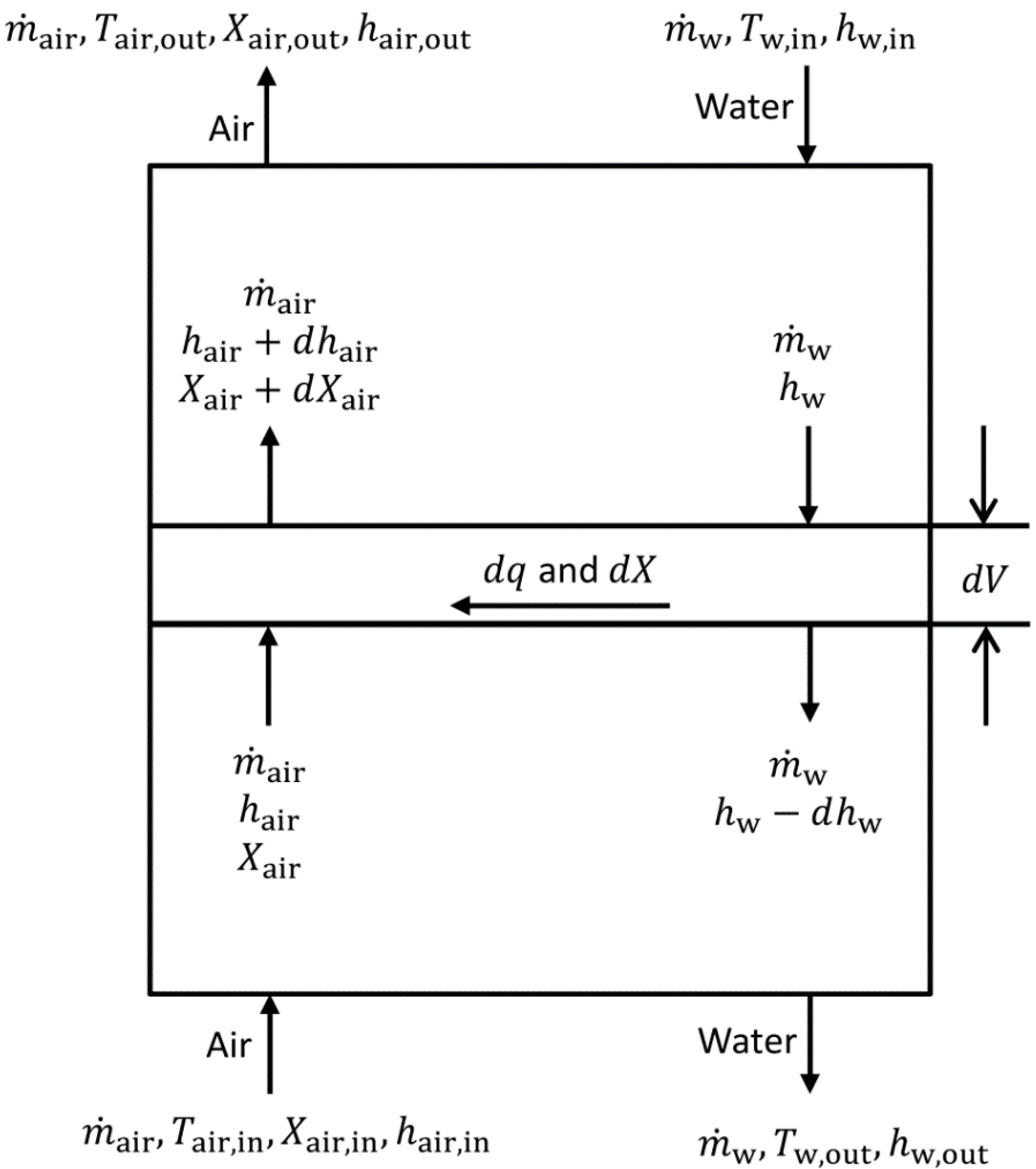
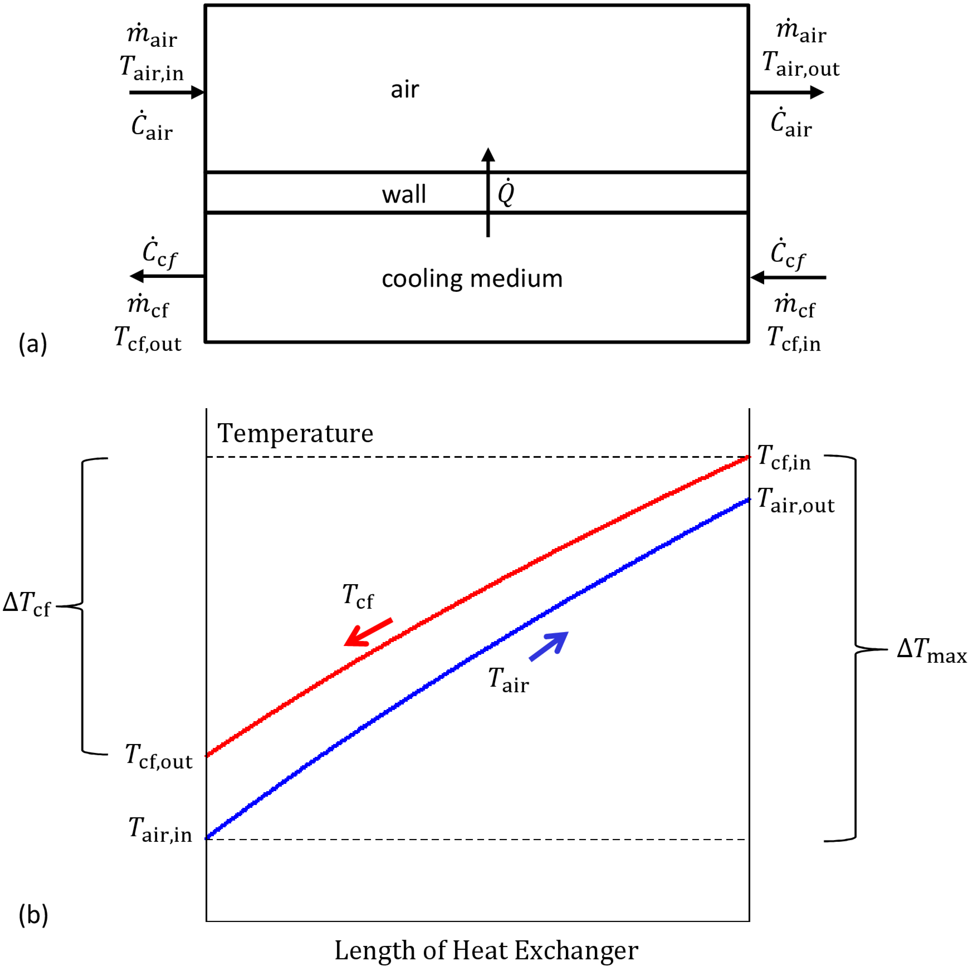
To depict this function explicitly, a detailed physical model or an extensive experimental study is required. However a reduction of parameters can be achieved without major losses in accuracy, as will be shown. The reduction is based on the effectiveness-NTU method, e.g., [12] and [13], which is based on the mass and energy balance of a heat exchanger, shown schematically in Figure 1. Therein the temperature effectiveness on cooling fluid side (${ϵ}_{\text{cf}}=\dot{Q}/({\dot{C}}_{\text{cf}}\text{ Δ}{T}_{\text{max}})$) is a function of the number of transfer units on air side (${\text{NTU}}_{\text{air}}=U A/{\dot{C}}_{\text{air}}$), the heat capacity rate ratio on cooling fluid side (${\dot{C}}_{\text{cf}}^{*}={\dot{C}}_{\text{cf}}/{\dot{C}}_{\text{air}}$) and the dry cooler configuration.

Figure 1. (a) Mass and energy balance of a counterflow dry cooler. (b) Scheme of temperatures over the length of the heat exchanger. The cooling effectiveness ${ϵ}_{\text{cf}}$ is defined by ${ϵ}_{\text{cf}}=\dot{Q}/({\dot{C}}_{\text{cf}}\text{ Δ}{T}_{\text{max}})$ and can be reformulated to due to ${ϵ}_{\text{cf}}=\text{Δ}{T}_{\text{cf}}/\text{Δ}{T}_{\text{max}}$ the energy balance $\dot{Q}={\dot{C}}_{\text{cf}}\text{ Δ}{T}_{\text{cf}}$.

Figure 1. (a) Mass and energy balance of a counterflow dry cooler. (b) Scheme of temperatures over the length of the heat exchanger. The cooling effectiveness ${ϵ}_{\text{cf}}$ is defined by ${ϵ}_{\text{cf}}=\dot{Q}/({\dot{C}}_{\text{cf}}\text{ Δ}{T}_{\text{max}})$ and can be reformulated to due to ${ϵ}_{\text{cf}}=\text{Δ}{T}_{\text{cf}}/\text{Δ}{T}_{\text{max}}$ the energy balance $\dot{Q}={\dot{C}}_{\text{cf}}\text{ Δ}{T}_{\text{cf}}$.

The heat capacity flow rates are defined as ${\dot{C}}_{\text{cf}}={\overline{c}}_{p,\text{cf} }{\dot{m}}_{\text{cf}}$ and ${\dot{C}}_{\text{air}}={\overline{c}}_{p,\text{air} }{\dot{m}}_{\text{air}}$, wherein the specific heat capacities are mean values with a dependency on fluid temperature, which has to be analyzed. The parameter $\text{Δ}{T}_{\text{max}}$ is the inlet temperature difference ($\text{Δ}{T}_{\text{max}}=T_{\text{cf},\text{in}}-T_{\text{air},\text{in}}$ in [K]). The temperature effectiveness ${ϵ}_{\text{cf}}$ will from now on be called cooling effectiveness. The cooling effectiveness ranges from zero to one. In an ideal HRU the cooling fluid would be cooled to the air inlet temperature, resulting in a value of ${ϵ}_{\text{cf}}$ equal to one with electric power as low as possible. The geometrical configuration is fixed for a given dry cooler, so ${ϵ}_{\text{cf}}$ can be written as a function of three parameters:

$${ϵ}_{\text{cf}}={ϵ}_{\text{cf}}({\text{NTU}}_{\text{air}},{\dot{C}}_{\text{cf}}^{*}, \text{DC})$$

(3)

Assuming that the overall heat transfer coefficient $U$ is a function of ${\dot{C}}_{\text{air}}$ and ${\dot{C}}_{\text{cf}}$ and the medium used as cooling fluid, ${\text{NTU}}_{\text{air}}$ and ${\dot{C}}_{\text{cf}}^{*}$ are given by:

$${\text{NTU}}_{\text{air}}= {\text{NTU}}_{\text{air}}({\dot{C}}_{\text{air}},{\dot{C}}_{\text{cf}},\text{DC},\text{cf})$$

(4)

$${\dot{C}}_{\text{cf}}^{*}= {\dot{C}}_{\text{cf}}^{*}({\dot{C}}_{\text{air}},{\dot{C}}_{\text{cf}})$$

(5)

This assumption is reasonable as long as the operating temperatures are within a limited range. In Table 1 the relevant properties of water, ethylene glycol based water solutions (30 Vol%) and air (relative humidity of 0%) for a temperature range of 20 to 45 °C (respectively 10 to 35 °C) are depicted.

Table 1. Thermodynamic properties of ethylene glycol solution, water and dry air at different temperatures (at 1 atm) and non-dimensional ratio between properties at the minimum temperature and the maximum temperature. Data calculated with CoolProp ([14] and [15]).

Medium	Range and Ratio	Thermal Conductivity (W/m K)	Dynamic Viscosity (10−5 kg/m s)	Density (kg/m³)	Specific Heat Capacity (103 J/kg K)
ethylene glycol solution	min (20 °C)	0.465	216.645	1038.046	3.718
	max (45 °C)	0.487	115.252	1026.153	3.789
	ratio	1.048	0.532	0.989	1.019
water	min (20 °C)	0.598	100.160	998.207	4.184
	max (45 °C)	0.635	59.577	990.213	4.18
	ratio	1.061	0.595	0.992	0.999
air	min (10 °C)	0.025	1.772	1.247	1.006
	max (35 °C)	0.027	1.893	1.146	1.007
	ratio	1.074	1.068	0.919	1.001

Table 1. Thermodynamic properties of ethylene glycol solution, water and dry air at different temperatures (at 1 atm) and non-dimensional ratio between properties at the minimum temperature and the maximum temperature. Data calculated with CoolProp ([14] and [15]).

Medium	Range and Ratio	Thermal Conductivity (W/m K)	Dynamic Viscosity (10−5 kg/m s)	Density (kg/m³)	Specific Heat Capacity (103 J/kg K)
ethylene glycol solution	min (20 °C)	0.465	216.645	1038.046	3.718
	max (45 °C)	0.487	115.252	1026.153	3.789
	ratio	1.048	0.532	0.989	1.019
water	min (20 °C)	0.598	100.160	998.207	4.184
	max (45 °C)	0.635	59.577	990.213	4.18
	ratio	1.061	0.595	0.992	0.999
air	min (10 °C)	0.025	1.772	1.247	1.006
	max (35 °C)	0.027	1.893	1.146	1.007
	ratio	1.074	1.068	0.919	1.001

In the air-conditioning and refrigeration industry, wet cooling towers are generally used in the range of 32 to 46 °C hot water temperature. A typical standard design condition for such cooling towers is 35 °C hot water to 29.4 °C cold water and 25.6 °C wet-bulb temperature [9].

The density difference in air due to different relative humidity is small in comparison to differences due to temperature changes (cf. [16]), therefore it will not be presented here. Differences in atmospheric pressure have a high impact on air density. Other properties in Table 1 are weakly affected when the pressure changes.

The Reynolds number (Re) and Prandtl number (Pr) of air as functions of the thermodynamic properties in Table 1 are slightly dependent on the temperature for constant capacity flow rate ${\dot{C}}_{\text{air}}$ and constant DC (differences of maximum to minimum Reynolds number are 6.8% with respect to maximum Reynolds number, due to temperature dependent dynamic viscosity differences). So the assumption that the heat transfer coefficient is only dependent on the capacity flow rate ${\dot{C}}_{\text{air}}$ and the dry cooler configuration DC is reasonable (especially as thermal conductivity is slightly increasing with temperature as well).

For the heat transfer coefficient of the cooling fluid side the dependency on temperature is much more pronounced, due to the strong effect of the temperature on viscosity. The differences in dynamic viscosity for a low mean temperature of 20 °C and a high mean temperature of 45 °C can be depicted by the relation of the viscosity, which is 0.53 for the ethylene glycol solution and 0.60 for water (cf. Table 1). To show the differences of heat transfer coefficients at low (${\text{α}}_{\text{cf},\text{low}}$) and high temperatures (${\text{α}}_{\text{cf},\text{high}}$) the relation is estimated by using the Dittus–Boelter correlation for turbulent flow in a smooth duct [13]. Therein the heat transfer for cooling is described by the Nusselt number:

$$\text{Nu}=0.026{\text{ Re}}^{0.8} {\text{Pr}}^{0.3}$$

(6)

The relation ${\text{α}}_{\text{cf},\text{low}}/{\text{α}}_{\text{cf},\text{high}}$ is calculated for the same geometry and equal capacity flow rates, resulting in a relation of 0.71 for the ethylene glycol solution and 0.64 for water. Although the difference seems not to be negligible, the overall heat transfer coefficient $U$ in a gas-to-liquid heat exchanger is typically determined by the gas side due to the much lower heat transfer coefficient. Assuming a dependency of cooling fluid side of 20% on $U$, a relative error of 29% (corresponding to ${\text{α}}_{\text{cf},\text{low}}/{\text{α}}_{\text{cf},\text{high}}=0.71$) for ${\text{α}}_{\text{cf}}$ yields an acceptable relative error in $U$ of 5.8%. Therefore Equation (4) is only weakly dependent on the temperature of the cooling fluid and thus this dependency will be ignored. Especially as in the estimation above two extreme values are compared to each other. Comparing one extreme value with a medium value (at water temperature of 32.5 °C) the relative error in U will further decrease. The relevance of the type of cooling fluid will be preserved, as the thermodynamic properties vary strongly from one cooling fluid to another. So on the one hand ${ϵ}_{\text{cf}}$ is, by definition:

$${ϵ}_{\text{cf}}=\frac{\dot{Q}}{{\dot{C}}_{\text{cf}}\text{ Δ}{T}_{\text{max}}}$$

(7)

On the other hand due to Equations (3)–(5) ${ϵ}_{\text{cf}}$ is given by a function $\text{ζ}$:

$${ϵ}_{\text{cf}}=\text{ζ}\left( {\dot{C}}_{\text{cf}},{\dot{C}}_{\text{air}},\text{DC},\text{cf}\right)$$

(8)

Taking the difference of Equations (7) and (8) yields a function $\text{τ}$:

$$\text{τ}\left({\dot{C}}_{\text{cf}},{\dot{C}}_{\text{air}},\text{DC},\text{cf},{ϵ}_{\text{cf}}\right)=\text{ζ}\left( {\dot{C}}_{\text{cf}},{\dot{C}}_{\text{air}},\text{DC},\text{cf}\right)-{ϵ}_{\text{cf}}$$

(9)

For measurement data $\tau$ is equal to zero, as the five parameters ${\dot{C}}_{\text{cf}}, {\dot{C}}_{\text{air}}, \text{DC},$$\text{cf}$ and ${ϵ}_{\text{cf}}$ are not independent of each other. In the mathematical formulation of Equation (9) the parameters are independent of each other and $\text{τ}$ can therefore be different from zero. Then the function $\text{τ}$ is only equal to zero if the choice of ${\dot{C}}_{\text{cf}}, {\dot{C}}_{\text{air}}, \text{DC}$ and $\text{cf}$ is in such a way that is corresponds to the choice of the fifth parameter ${ϵ}_{\text{cf}}$ in the function $\text{τ}$. Therefore ${\dot{C}}_{\text{air}}$ might be partly given by an implicit function $\varphi$:

$${\dot{C}}_{\text{air}}=\varphi \left( {ϵ}_{\text{cf}}, {\dot{C}}_{\text{cf}}, \text{DC},\text{cf}\right)$$

(10)

The function $\varphi$ will not be defined for every possible choice of $\left({ϵ}_{\text{cf}}, {\dot{C}}_{\text{cf}}, \text{DC},\text{cf}\right)$, but it can be shown with the implicit function theorem [17], that if there exists one value for ${\dot{C}}_{\text{air}}$ and fixed values for $\left({ϵ}_{\text{cf}}, {\dot{C}}_{\text{cf}}, \text{DC},\text{cf}\right)$, such that $\text{τ}\left({\dot{C}}_{\text{cf}},{\dot{C}}_{\text{air}},\text{DC},\text{cf},{ϵ}_{\text{cf}}\right)=0$, the function $\varphi$ is defined in a neighbourhood around $\left({ϵ}_{\text{cf}}, {\dot{C}}_{\text{cf}}, \text{DC},\text{cf}\right)$. A necessary condition for validity of the implicit function theorem is that ${\frac{\partial \text{τ}}{\partial {\dot{C}}_{\text{air}}}|}_{{ϵ}_{\text{cf}}, {\dot{C}}_{\text{cf}}, \text{DC},\text{cf}}\ne 0$ at these fixed values. The proof is based on the idea, that the function $\text{τ}$ in Equation (9) is a monotonously increasing function of ${\dot{C}}_{\text{air}}$ and only in $\text{ζ}$ dependent on ${\dot{C}}_{\text{air}}$.

Therefore ${\frac{\partial \text{τ}}{\partial {\dot{C}}_{\text{air}}}|}_{{ϵ}_{\text{cf}}, {\dot{C}}_{\text{cf}}, \text{DC},\text{cf}}={\frac{\partial \text{ζ}}{\partial {\dot{C}}_{\text{air}}}|}_{{ϵ}_{\text{cf}}, {\dot{C}}_{\text{cf}}, \text{DC},\text{cf}}= {\frac{\partial \text{ζ}}{\partial {\dot{C}}_{\text{air}}}|}_{{\dot{C}}_{\text{cf}}, \text{DC},\text{cf}}>0$, as it is obvious, that for an increasing capacity flow rate on air side (respectively increasing air mass flow rate) and constant capacity flow rate on water side (respectively constant water mass flow rate) the function $\text{ζ}$ for cooling effectiveness will increase in a given dry cooler. Therefore ${\frac{\partial \text{τ}}{\partial {\dot{C}}_{air}}|}_{{ϵ}_{\text{cf}},{\dot{\text{C}}}_{\text{cf}}, \text{DC},\text{cf}}\ne 0$ holds (cf. Equation (9)), a necessary and sufficient requirement for the implicit function theorem. For the studied monitoring data Equation (10) is always applicable, however an extrapolation of Equation (10) for other parameters might not exist.

The relationship of Equation (10) for a simulated exemplary dry cooler (with a similar configuration as the dry cooler DC1 which will be presented in the subsequent Section 3) is shown in Figure 2. The figure shows that the four parameters ${ϵ}_{\text{cf}}, {\dot{C}}_{\text{cf}}, \text{DC}$ and $\text{cf}$ have strong influence on the air heat capacity flow rate ${\dot{C}}_{\text{air}}$, whereas the influence of temperature on ${\dot{C}}_{\text{air}}$ is minor. The air heat capacity flow rate is an increasing function of cooling effectiveness, with a vertical asymptote less than or equal to one.

In Figure 2a two different cooling fluids are used for simulation. The cooling fluid heat capacity flow rate is constant and equal for the cooling fluids, as well as the dry cooler flow configuration and the inlet temperatures on the cooling fluid and air side. For a fixed cooling effectiveness the difference in air heat capacity flow rate is up to 10% and therefore not negligible. Figure 2b,c show a similar result, with a strong influence of the changing parameters ${\dot{C}}_{\text{cf}}$ and flow configuration on the curve. The flow configuration in Figure 2c is altered just be changing the number of passes on the water side. For different inlet temperatures (Figure 2d,e) and for a fixed cooling effectiveness the difference in air heat capacity flow rate is less 4%. This approves the proceeding not to consider the dependency on temperature in the implicit function $\varphi$ in Equation (10).

Figure 2. Dependency of cooling fluid capacity flow rate versus cooling effectiveness on different parameters. Other parameters than the changed parameters are constant. Further explanation is given in the text. (a) Changing the cooling fluid; (b) Changing the cooling fluid heat capacity flow rate; (c) Changing the dry cooler flow configuration; (d) Changing cooling fluid inlet temperature; (e) Changing air inlet temperature.

Figure 2. Dependency of cooling fluid capacity flow rate versus cooling effectiveness on different parameters. Other parameters than the changed parameters are constant. Further explanation is given in the text. (a) Changing the cooling fluid; (b) Changing the cooling fluid heat capacity flow rate; (c) Changing the dry cooler flow configuration; (d) Changing cooling fluid inlet temperature; (e) Changing air inlet temperature.

2.1. Electric Power for Fans

Assuming that the electrical consumption for the fans $P_{\text{el},\text{Fan}}$ is dependent on the mass flow rate of air only (ignoring the impact of temperature dependent density and viscosity), $P_{\text{el},\text{Fan}}$ is dependant on ${\dot{C}}_{\text{air}}$ only, as the heat capacity variation of air in the given temperature range (cf. Table 1) is negligible. The fan is fixed as one part of the dry cooler. Due to Equation (10) it is:

$$P_{\text{el},\text{Fan}}= P_{\text{el},\text{Fan}}\left({ϵ}_{\text{cf}}, {\dot{C}}_{\text{cf}}, \text{DC},\text{cf}\right)$$

(11)

This simplification is necessary if later electric powers have to be compared without knowledge of temperatures at operation. In general the electric power is calculated by $P_{\text{el},\text{Fan}}=\left(\text{Δ}{p}_{\text{air}}{\dot{m}}_{\text{air}}\right)/({\text{ρ}}_{\text{air}}{\text{η}}_{\text{Fan}})$, with fan efficiency ${\text{η}}_{\text{Fan}}$. Therefore a more precise assumption is to include a temperature dependent density in the calculation. For two different temperatures the ratio between the electric power for fans necessary to run an equal air capacity flow rate (and assuming $c_{p,\text{air},\text{ low}}=c_{p,\text{air},\text{ high}}$) is given by:

$$\frac{P_{\text{el},\text{Fan},\text{low}}}{P_{\text{el},\text{Fan},\text{high}}}=\frac{f_{\text{low}}}{f_{\text{high}}}{\left(\frac{{\text{ρ}}_{\text{air},\text{high}}}{{\text{ρ}}_{\text{air},\text{low}}}\right)}^2\frac{{\text{η}}_{\text{Fan},\text{high}}}{{\text{η}}_{\text{Fan},\text{low}}}$$

(12)

where the friction factor $f_{\text{low}}$ (respectively $f_{\text{high}}$) is a function of Reynolds number and therefore dependent on the dynamic viscosity of air at a given temperature. As the relationship between friction factor and Reynolds number is different for all types of heat exchangers, it is not possible to develop a generally valid expression of $f_{\text{low}}/f_{\text{high}}$ in terms of Reynolds numbers. The correlations given in literature are mostly based on the formula $f=c_1 {\text{Re}}^{c_2}$, with $c_1$ and $c_2$ being constants dependent on geometry. For a flow through a staggered tube bundle $c_2$ is in the range of $-1$ to $-0.25$ [18]. A good overview for correlations of complex geometries is given in [13] (e.g., Offset Strip Fins, Louver Fins, Individually Finned Tubes, Plain Flat Fins and Corrugated Flat Fins on a Tube Array, Cross rod geometries). For an equal air capacity flow rate at different temperatures (${\dot{C}}_{\text{air},\text{low}}={\dot{C}}_{\text{air}, \text{high}}$) and a constant heat exchanger geometry the ratio of Reynolds numbers is equal to the inverse ratio of dynamic viscosities $\text{η}$, as heat capacity of air is constant for different temperatures (cf. Table 1). Using the basic formula for friction factor to Reynolds number correlations yields:

$$\frac{f_{\text{low}}}{f_{\text{high}}}={\left(\frac{{\text{Re}}_{\text{low}}}{{\text{Re}}_{\text{high}}}\right)}^{c_2} ={\left(\frac{{\text{η}}_{\text{high}}}{{\text{η}}_{\text{low}}}\right)}^{c_2}$$

(13)

This ratio is equal to 0.95 (respectively 0.99) for $c_2=-1$ (respectively $c_2=-0.25$). We will therefore in the following analysis neglect the ratio of friction factors in Equation (12), accepting an error of 5% in the equation. On the differences of fan efficiency ${\text{η}}_{\text{Fan}}$ at different temperatures, but equal air capacity flow rates, such a general statement is not possible. Nevertheless as ambient temperatures during operation will be in a restricted range, we will ignore fan efficiency differences due to temperature differences.

Considering a mean temperature of inlet air of 25 °C (cf. standard in [6]) Equation (12) can then be reformulated to:

$$P_{\text{el},\text{Fan},25°\text{C}}={\left(\frac{{\text{ρ}}_{\text{air}}}{{\text{ρ}}_{\text{air},25°\text{C}}}\right)}^2\cdot P_{\text{el},\text{Fan}}$$

(14)

The measured data $P_{\text{el},\text{Fan}}$ (and ${\text{ρ}}_{\text{air}}$) at an inlet air temperature different to 25 °C is thus transformed to a standardized electric power $P_{\text{el},\text{Fan},25°\text{C}}$. The negligence of density differences of air due to temperature differences in Equation (11) is therefore not necessary anymore, if the electric power of fans is calculated as follows:

$$P_{\text{el},\text{Fan},25°\text{C}}\left({ϵ}_{\text{cf}}, {\dot{C}}_{\text{cf}}, \text{DC},\text{cf}\right)= {\left(\frac{{\text{ρ}}_{\text{air}}}{{\text{ρ}}_{\text{air},25°\text{C}}}\right)}^2\cdot P_{\text{el},\text{Fan}}\left({ϵ}_{\text{cf}}, {\dot{C}}_{\text{cf}}, \text{DC},\text{cf}\right)$$

(15)

The density ${\text{ρ}}_{\text{air},25 °C}$ is at standard ambient pressure of 1013.25 hPa for dry air. Differences in atmospheric pressure and relative humidity on density of air are included in Equation (15).

2.2. Electric Power for Pump

The electrical consumption for the pump $P_{\text{el},\text{Pump}}$ can be approximated by the capacity flow rate of cooling fluid; however the temperature of cooling fluid cannot be ignored, due to strong dependency of pressure drop on viscosity. Using the Blasius equation [13] for turbulent flow in a smooth duct the dissipated power ($P_{\text{Diss}}={\dot{m}}_{\text{cf}}\text{Δ}{p}_{\text{cf}}/{\text{ρ}}_{\text{cf}})$ on the cooling fluid side can be calculated exemplarily. The relation of dissipated energy at low temperature $P_{\text{Diss},\text{cf},\text{low} }$ to dissipated energy at high temperature $P_{\text{Diss},\text{cf},\text{high} }$ of the cooling fluid (cf. Table 1) is then given by:

$$\frac{P_{\text{Diss},\text{cf},\text{low} }}{P_{\text{Diss},\text{cf},\text{high} }}={\left(\frac{{\dot{C}}_{\text{cf}, \text{low}}}{{\dot{C}}_{\text{cf}, \text{high}}}\right)}^{0.75}{\left(\frac{c_{p,\text{cf}, \text{low}}}{c_{p,\text{cf}, \text{high}}}\right)}^{-0.75}{\left(\frac{{\text{η}}_{\text{cf},\text{ low}}}{{\text{η}}_{\text{cf},\text{ high}}}\right)}^{0.25},$$

(16)

as the geometric parameters are constant.

Considering equal capacity flow rates yields $P_{\text{Diss},\text{cf},\text{low} }/P_{\text{Diss},\text{cf},\text{high} }=0.84$ for ethylene glycol solution and $P_{\text{Diss},\text{cf},\text{low} }/P_{\text{Diss},\text{cf},\text{high} }=0.88$ for water. Following the same idea as for the electric power for fans, a mean cooling fluid temperature of 40 °C is defined (cf. standard in [6]). Neglecting the ratio of heat capacities in Equation (16) and assuming that pump efficiency due to temperature differences of the cooling fluid can be neglected, the electric power for the pump at 40 °C is:

$$P_{\text{el},\text{Pump},40°\text{C}}\left({\dot{C}}_{\text{cf}},\text{DC},\text{cf}\right)= {\left(\frac{{\text{η}}_{\text{cf}, 40°\text{C}}}{{\text{η}}_{\text{cf}}}\right)}^{0.25}\cdot P_{\text{el},\text{Pump}}\left({\dot{C}}_{\text{cf}},\text{DC},\text{cf}\right)$$

(17)

The measured data $P_{\text{el},\text{Pump}}$ at an inlet air temperature different to 40 °C is thus transformed to a standardized electric power $P_{\text{el},\text{Pump},40°\text{C}}$, using a correction factor based on the differences in dynamic viscosity due to temperature differences. A total standardized electric power $P_{\text{el},25°\text{C},40 °\text{C}}$ is then calculated to be:

$$P_{\text{el},25°\text{C},40°\text{C}}\left({ϵ}_{\text{cf}}, {\dot{C}}_{\text{cf}}, \text{DC},\text{cf}\right)=P_{\text{el},\text{Fan},25°\text{C}}\left({ϵ}_{\text{cf}}, {\dot{C}}_{\text{cf}}, \text{DC},\text{cf}\right)+ P_{\text{el},\text{Pump},40°\text{C}}\left({\dot{C}}_{\text{cf}},\text{DC},\text{cf}\right)$$

(18)

Monitored and simulated data of electric power at temperatures within a specified range (cf. Table 1) can thus be transformed with Equation (18) to a comparable value for electric power.

Summing up, a functional relationship between operating conditions (expressed by ${ϵ}_{\text{cf}}$ and ${\dot{C}}_{\text{cf}}$) as well as geometrical and system configuration ($\text{DC}$ and $\text{cf}$) and the electrical power demand to operate the heat rejection unit has been developed. This method is based on two validated models describing thermodynamic relationships, first the NTU method and second the determination of electrical power demand based on fan/pump efficiency. The method above merges the two models to one method, describing the cost of heat rejection units in terms of electrical power and the benefit in terms of cooling effectiveness.

3. Monitoring Data and Simulation of Dry Coolers

For the comparison of various types of dry coolers and the evaluation of measurement data this approach enables us to describe the electric power needed to run pumps and fans for a given dry cooler and a cooling fluid in use by solely knowing the value of ${\dot{C}}_{\text{cf}}$ and ${ϵ}_{\text{cf}}$ as described in Equation (18). Further knowledge on temperatures to determine air density and cooling fluid viscosity will increase the accuracy. As the systems for solar cooling differ, so does the method to determine monitoring data. This results in a non-uniform definition of electric power for the HRU. In Figure 3 different system boundaries for electric powers are defined.

The first boundary (B1) includes only the electric power $P_{\text{el},\text{Fan}}$ necessary to run the fan. If simulation data is used, the electric power for the fan is calculated by the quotient of dissipated energy ($P_{\text{Diss},\text{air}}={\dot{V}}_{\text{air}}\text{Δ}{p}_{\text{air}})$ and an assumed average fan efficiency of ${\text{η}}_{\text{Fan}}=0.5$ (this value is equal to 150% of the minimum fan efficiency in the energy efficiency requirements for axial fans with electrical power input of 0.8 kW (cf. [19]). The second boundary (B2) includes the electric powers from B1 plus the fraction of electric power for the cooling fluid pump needed to overcome the pressure drop on the fluid side of the dry cooler (not the tubes connecting chiller and dry cooler). For simulation data this fraction is given by ${\dot{V}}_{\text{cf}}\text{Δ}{p}_{\text{cf}}/{\text{η}}_{\text{Pump}}$, with ${\text{η}}_{\text{Pump}}=0.3$. In B3 the whole electric power for the cooling fluid pump is taken into account, additional to the electric power for the fan (B1). Some dry coolers operate with a second heat exchanger, separating the cooling fluid (e.g., ethylene glycol solution) from the water in the chiller.

Figure 3. System boundaries for electric power in monitoring projects. Boundary 1 includes the electric power input of the fans on the air side only. All other boundaries include in addition a fraction of or the total electric power input of the pumps on the cooling fluid and water side.

Figure 3. System boundaries for electric power in monitoring projects. Boundary 1 includes the electric power input of the fans on the air side only. All other boundaries include in addition a fraction of or the total electric power input of the pumps on the cooling fluid and water side.

The electric power needed to run this second pump is added in B4 to the power needed in B3. An increased cooling water temperature after the heat exchanger is measured in this case. However determination of cooling effectiveness in this paper will always be based on temperatures in the cooling fluid circle, not in the water circle to the chiller. If this data is not available an estimation of temperature reduction in the second heat exchanger takes place. The monitoring data which will be analyzed does not contain information on all of these boundaries. A comparison of different dry coolers should take place only within the same boundary. In the following, data from seven sources were used to depict the performance graphically, according to Equations (2), (15) and (18):

• DC1: Data calculated with the software CoilDesigner [20] for a dry cooler ($A_{\text{HTS}}=152 \text{m}²)$; air and cooling fluid (water) mass flow rate as well as both inlet temperatures are varied; data for B1 and B2 is given;
• DC2: set of monitoring data from the German project SolCoolSys [21] ($A_{\text{HTS}}$ unknown); air mass flow rate and both inlet temperatures are varied; The dry cooler is operated with an ethylene glycol solution (approximately 30 Vol%), the heat capacity is measured in the water circuit after a separating heat exchanger; temperatures for the cooling fluid side are calculated by assuming an effective temperature difference of 1.5 K in the separating heat exchanger; data for B1, B3 (temperatures calculated) and B4 is given;
• DC3: set of monitoring data from the German project SolCoolSys [21] with a more recent dry cooler model than DC2 ($A_{\text{HTS}}=221 \text{m}²)$; same system as DC2; data for B1, B3 (temperatures calculated) and B4 is given;
• DC4: Lab data measured by German manufacturer Thermofin [22] for a dry cooler ($A_{\text{HTS}}=46 \text{m}²)$; air and cooling fluid (water) mass flow rate as well as both inlet temperatures are varied; data for B1 and B2 is given;
• DC5: set of monitoring data from the German project SolCoolSys [21] ($A_{\text{HTS}}=221 \text{m}²)$; air mass flow rate and both inlet temperatures are varied; the dry cooler is operated with an ethylene glycol solution (30 Vol%) as cooling fluid; temperatures are measured in the cooling fluid circuit and in the water circuit after a separating heat exchanger; data for B1, B3 and B4 is given;
• DC6: Data calculated with the software Güntner Product Calculator [23] for a dry cooler with axial fans and multiple-row line-up (type GFW, $A_{\text{HTS}}=1072 \text{m}²)$; air and cooling fluid (water) mass flow rate as well as both inlet temperatures are varied; data for B1 is given;
• DC7: set of monitoring data by the Bavarian Center for Applied Energy Research (ZAE Bayern) [24]; The dry cooler with axial fans is assembled horizontally and produced by Güntner (type GFH, $A_{\text{HTS}}=197 \text{m}²)$; air and cooling fluid (water) mass flow rate as well as both inlet temperatures are varied; data for B1 is given.

The simulated and monitored HRU were largely operated at a constant cooling fluid mass flow rate and therefore at a constant cooling fluid capacity flow rate. The ratio between ${\dot{C}}_{\text{cf}}$ and the heat transfer surface (HTS) of the heat exchangers describes the type of operation. A low value of cooling fluid capacity flow rate at a high value of HTS may be an indication for high investment cost, compared to operation cost, as a larger heat exchanger has to be installed if a certain heat flow rate shall be achieved. However the cost for electric power for fans is reduced, as the HTS is large. In Figure 4 the cooling fluid capacity flow rate and the heat transfer surface of DC1 to DC7 are shown.

Figure 4. Differences of size and operating conditions of simulated and monitored dry coolers, expressed by heat transfer surface (HTS) and cooling fluid capacity flow rate (${\dot{C}}_{\text{cf}})$. Areas of same grey coloration correspond to same ratio of ${\dot{C}}_{\text{cf}}$ and HTS.

Figure 4. Differences of size and operating conditions of simulated and monitored dry coolers, expressed by heat transfer surface (HTS) and cooling fluid capacity flow rate (${\dot{C}}_{\text{cf}})$. Areas of same grey coloration correspond to same ratio of ${\dot{C}}_{\text{cf}}$ and HTS.

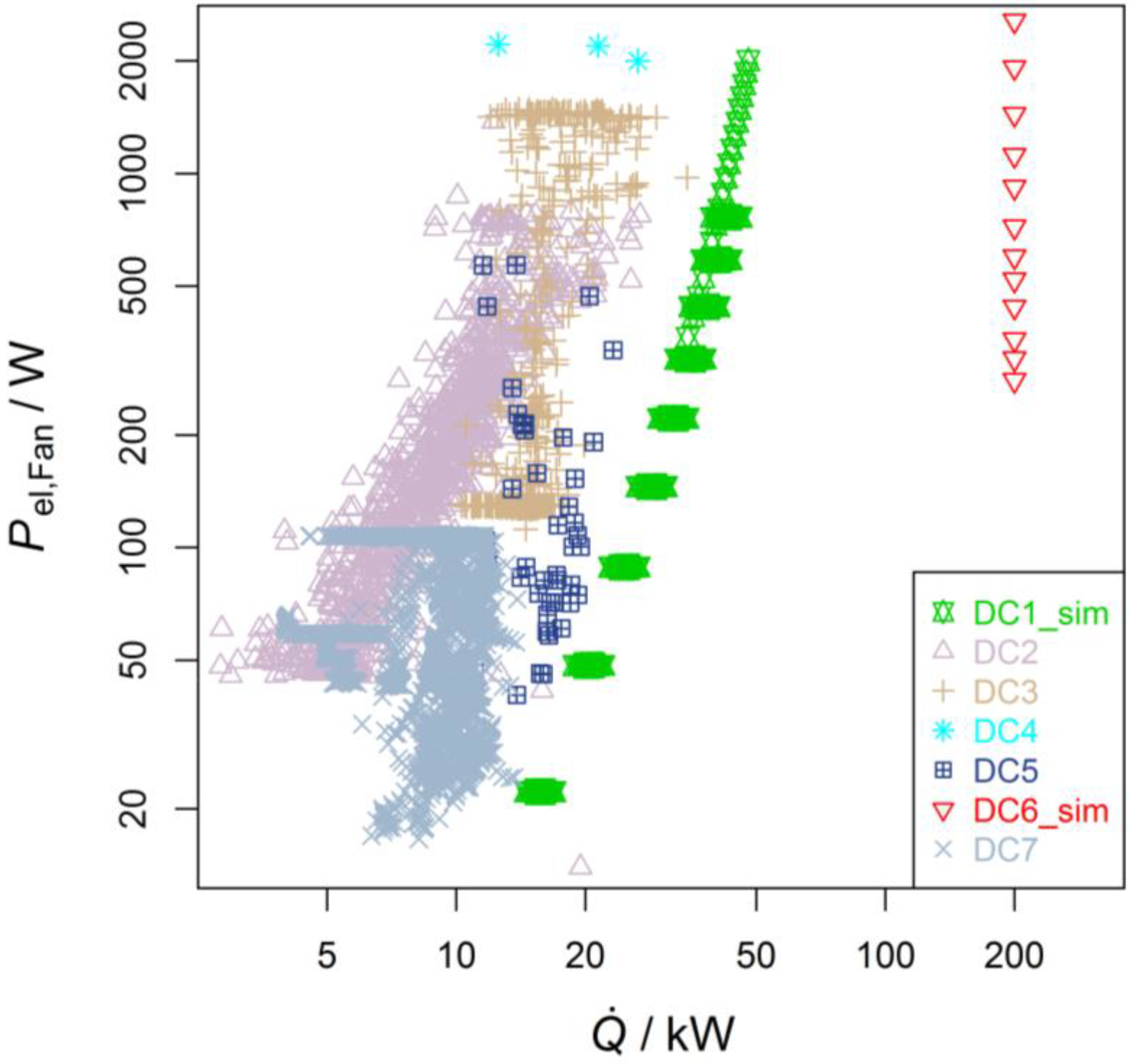
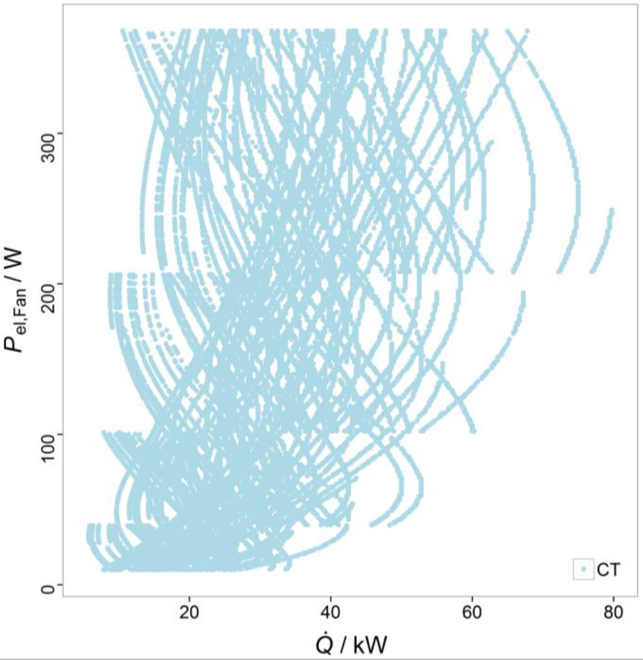
It is to be expected that DC4 has a high electricity demand, as the capacity flow rate is high in relation to the available HTS. Further DC5 und DC7 should show a better thermodynamic performance. In Figure 5 a general depiction of performance is shown. The electric power for fans is plotted versus heat flow rate. According to Equation (2) the electric power is further dependent on temperatures. This dependency is not included in this plot. The good performance of DC1 and DC6 (high $\dot{Q}$ at low $P_{\text{el},\text{Fan}}$) is at least partly due to a larger driving temperature difference between the two fluids. An evaluation of performance based on this plot is not possible.

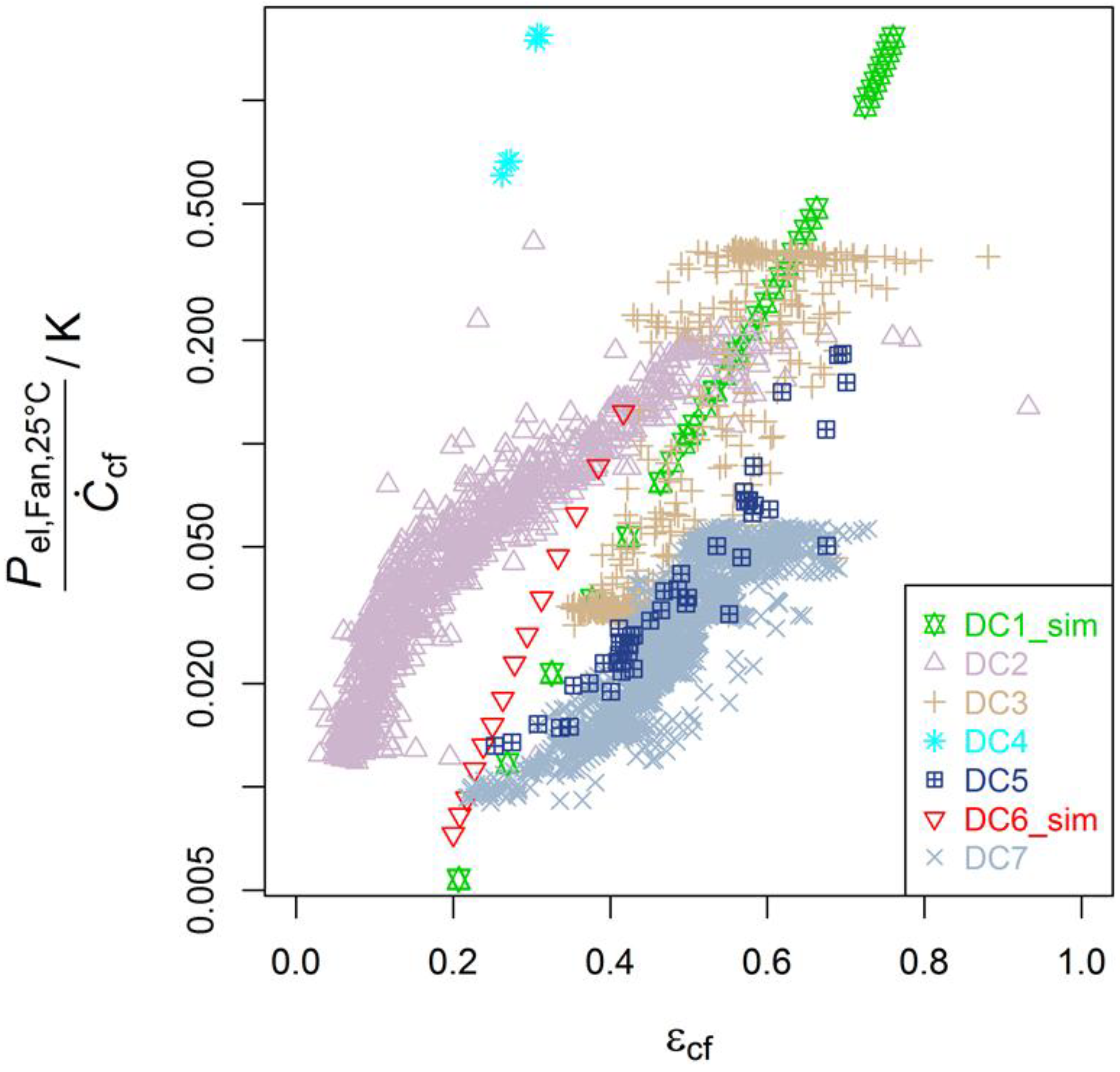
In Figure 6 the electric power for fans at 25 °C is normalized with the cooling fluid capacity flow rate. This specific electric power demand is plotted versus cooling effectiveness, according to Equation (15). The reason for normalizing the electric power demand is to compare different sized HRU with each other. A performance evaluation based on Figure 6 yields for every cooling ratio a best HRU. For example, at ${ϵ}_{\text{cf}}=0.3$ DC7 has the lowest specific electric power demand, DC4 the highest. At ${ϵ}_{\text{cf}}=0.2$ DC1 is better than DC7. Ignoring the scattering of monitoring data, each dry cooler can be represented by a curve. The courses of the curves are similar, ranging from a straight line in the log-plot to a slightly bended curve, as an increase in cooling effectiveness can only be achieved when increasing the air volume flow and therefore the electric power for fans.

Figure 5. Electric power for fans ($P_{\text{el},\text{Fan}}$) versus rejected heat ($\dot{Q}$) for simulated and monitored dry coolers (in boundary B1). This depiction is not suitable to compare performance of HRU.

Figure 5. Electric power for fans ($P_{\text{el},\text{Fan}}$) versus rejected heat ($\dot{Q}$) for simulated and monitored dry coolers (in boundary B1). This depiction is not suitable to compare performance of HRU.

Figure 6. Electric power for fans at 25 °C ($P_{\text{el},\text{Fan},25°\text{C}}$) normalized with cooling fluid capacity flow rate versus cooling effectiveness (${ϵ}_{\text{cf}})$ for simulated and monitored dry coolers (in boundary B1).

Figure 6. Electric power for fans at 25 °C ($P_{\text{el},\text{Fan},25°\text{C}}$) normalized with cooling fluid capacity flow rate versus cooling effectiveness (${ϵ}_{\text{cf}})$ for simulated and monitored dry coolers (in boundary B1).

The information given in the plot is diverse; however two findings shall be touched upon. First DC2 has been replaced by DC3 during monitoring. The improvement is evident: a three-fold decrease of the specific electric power for fans at a cooling effectiveness of ${ϵ}_{\text{cf}}=0.4$ (from 0.1 $W_{\text{el}}/(W_{\text{th}}/K)$ for DC2 to 0.03 $W_{\text{el}}/(W_{\text{th}}/K)$ for DC3) and further an increase in cooling effectiveness during operation from a range of ${ϵ}_{\text{cf}}=$ (0.1,0.5) to ${ϵ}_{\text{cf}}=$ (0.4,0.7). Second the dry coolers DC3 and DC5 are the same type of cooler, but operated at different locations and different cooling fluid mass flow rates. DC5 shows a better performance within the total range of cooling effectiveness, e.g., the specific electric power for fans at ${ϵ}_{\text{cf}}=0.4$ is only 66% of DC3.

To determine the electric power for fans for a specific rate of heat flow $\dot{Q}$ and a specific temperature driving force $\text{Δ}{T}_{\text{max}}$, the cooling effectiveness has to be calculated first with Equation (7), based on the cooling fluid capacity flow rate used in Figure 6. Then the electric power demand can be determined from the curves in the plot.

The following sample calculation is intended to clarify the application of Figure 6. Assuming $\dot{Q}=20\text{ kW}$, ${\text{ΔT}}_{\text{max}}=10 \text{K}$ and a cooling fluid capacity flow rate of ${\dot{C}}_{\text{cf}}=4000 \text{W}/\text{K}$ Equation (7) yields a cooling effectiveness of ${ϵ}_{\text{cf}}=0.5$. The required cooling fluid capacity flow rate can, e.g., be realized with DC2 or with two devices of DC7 (based on the data). The specific electric power demand for DC2 is approximately $0.09 {\text{W}}_{\text{el}}/({\text{W}}_{\text{th}}/\text{K})$, for DC7 it is $0.03 {\text{W}}_{\text{el}}/({\text{W}}_{\text{th}}/\text{K})$. As ${\dot{C}}_{\text{cf}}$ is equal for both applications the electric power for fans is three times higher for DC2 (360 W) than for two devices of DC7 (120W). However the heat transfer surface is doubled for the two devices of DC7, resulting probably in higher investment cost for application of DC7 at this operating point.

The difference between plotting electric power for fans at 25 °C (Equation (15)) and at the monitored ambient temperatures (Equation (11)) is marginal with $\pm 2.6\%$. The scattering of monitoring data is due to a transient heat transfer process and a non-constant value for cooling fluid capacity flow rate (limited to a certain range) to increase the usable data points.

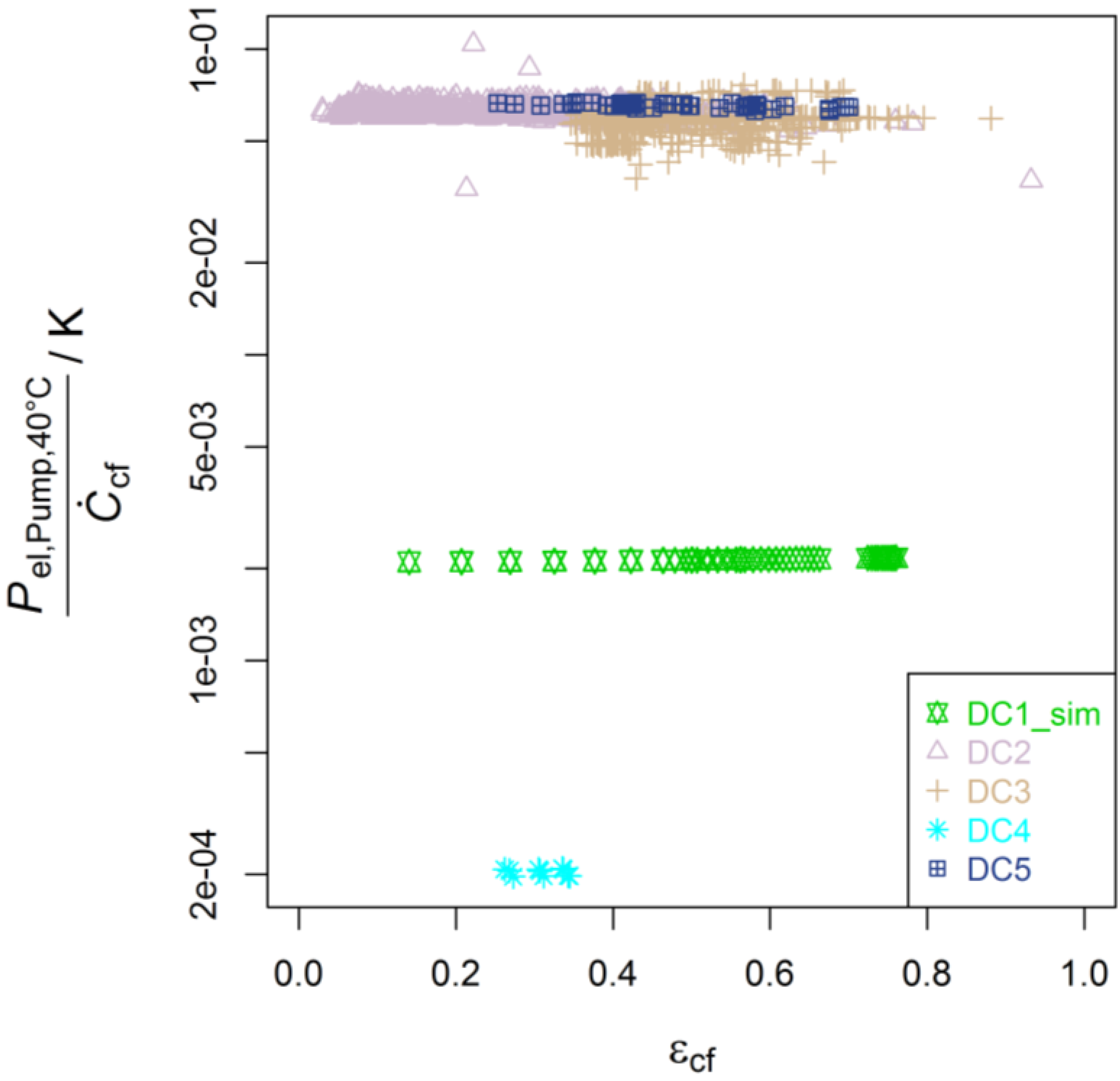
In Figure 7 the specific electric power for the pump versus the cooling effectiveness (cf. Equation (17)) is depicted. As the cooling fluid capacity flow rate is constant the electric power is almost constant (cf. Equation (16)). The values for specific electric power for the pump range from $0.2 {\text{W}}_{\text{el}}/({\text{kW}}_{\text{th}}/\text{K})$ to $10 {\text{W}}_{\text{el}}/({\text{kW}}_{\text{th}}/\text{K})$. The difference in demand of the dry coolers is due to the specific fraction of electric power that is used in this calculation. For DC1 and DC4 the fraction of B2 is taken (without B1). For DC2, DC3 and DC5 boundary B3 (without B1) is taken into account. No information on electric power for pumps was available for DC6 and DC7. Further the differences in cooling fluid capacity flow rate yield a higher value of specific electric power for the pump for DC1 (compared to DC4).

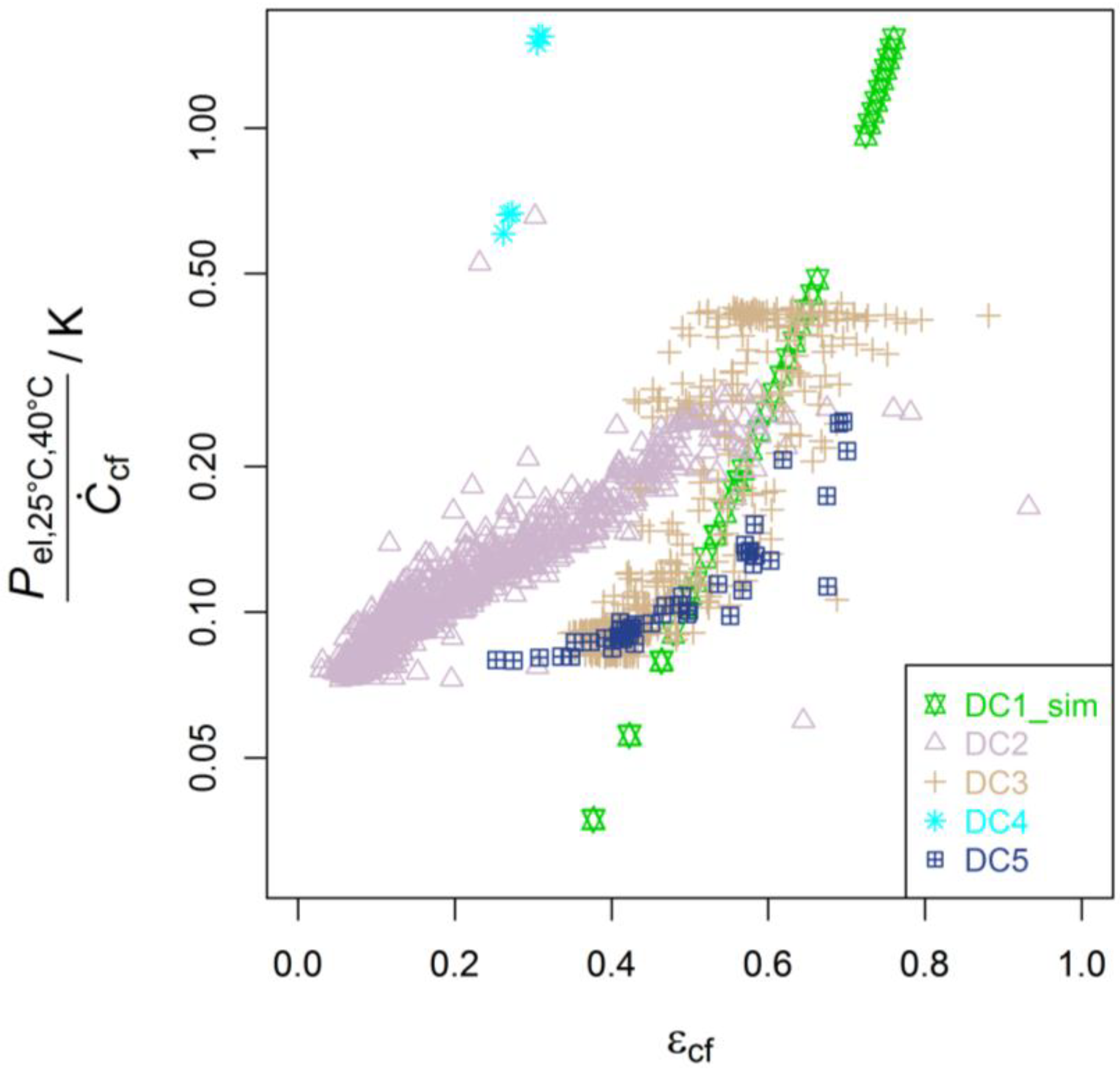
Adding the values in Figure 6 and Figure 7 yields a specific electric power for the HTU (cf. Equation (18)). This is depicted in Figure 8. The fraction of electric power for the pump of the entire electrical demand is between 50% and 80% for DC2, DC3 and DC5 (dependent on cooling effectiveness). Therefore at lower cooling effectiveness the differences between the three DCs is less dominant than in Figure 6. A Comparison to DC1 and DC4 is possible only to a limited extent as the electric power for pumps are within different system boundaries for electric power.

The validity of the method is shown in particular by the unique functional relationship for the simulated data in Figure 6 and Figure 8, which reveals no scattering at all.

Figure 7. Electric power for pump at 40 °C ($P_{\text{el},\text{Pump},40°\text{C}}$) normalized with cooling fluid capacity flow rate versus cooling effectiveness (${ϵ}_{\text{cf}}$) for simulated and monitored dry coolers (DC1 and DC4 in boundary B2 and DC2, DC3 and DC5 in B3; Excluding B1).

Figure 7. Electric power for pump at 40 °C ($P_{\text{el},\text{Pump},40°\text{C}}$) normalized with cooling fluid capacity flow rate versus cooling effectiveness (${ϵ}_{\text{cf}}$) for simulated and monitored dry coolers (DC1 and DC4 in boundary B2 and DC2, DC3 and DC5 in B3; Excluding B1).

Figure 8. Electric power for fans and pump at 25 °C and 40 °C ($P_{\text{el},25°\text{C},40°\text{C}}$) normalized with cooling fluid capacity flow rate versus cooling effectiveness (${ϵ}_{\text{cf}})$ for simulated and monitored dry coolers (DC1 and DC4 in boundary B2 and DC2, DC3 and DC5 in B3).

Figure 8. Electric power for fans and pump at 25 °C and 40 °C ($P_{\text{el},25°\text{C},40°\text{C}}$) normalized with cooling fluid capacity flow rate versus cooling effectiveness (${ϵ}_{\text{cf}})$ for simulated and monitored dry coolers (DC1 and DC4 in boundary B2 and DC2, DC3 and DC5 in B3).

In this study we will not present a method to combine investment cost (related strongly to size of heat transfer surface, cf. Figure 4) and operation cost (related strongly to electricity demand) to one parameter characterizing total cost, as additional information on operating conditions over the entire operational lifetime have to be given. These conditions vary strongly from system to system and total cost has to be calculated in the individual case. The advantage of the depiction in Figure 6 to Figure 8 is that all necessary information for changing operating conditions are included and operation cost for pumps and fans can easily be calculated if the operating conditions over the entire operational lifetime are given and converted to cooling efficiency. Different designs and configuration of heat rejection units can only be judged on the level of combined investment and operating costs, otherwise if ignoring investment cost, a heat exchanger with very large heat transfer surface would be preferable. Nevertheless the depiction method described above shows the difference in operation cost due to electricity demand for different designs and offers a possibility to compare the investment cost due to size of heat transfer surface (cf. Figure 4).

4. Wet Cooling Towers

The effectiveness-NTU method is generally applied for heat exchanger based on sensible heat transfer. Yet in the following chapter it will be shown, that a similar method as the one used for dry coolers above can be derived for wet cooling towers. Due to the lack of appropriate monitoring data, the method is only developed theoretically and not yet applied to measured data.

To start with, the following assumptions are adopted from [25]:

• Heat and mass transfer is in a direction normal to the flows only;
• Negligible heat and mass transfer through the tower walls to the environment;
• Negligible heat transfer from the tower fans to the air or water streams;
• Constant water and dry air specific heats;
• Constant heat and mass transfer coefficients throughout the tower;
• Value of Lewis number equal to unity;
• Water loss due to evaporation is negligible (constant ${\dot{m}}_{\text{w}}$);
• Uniform temperature throughout the water stream at each cross section;
• Uniform cross sectional area of the tower.

In Figure 9 a counterflow wet cooling tower is shown schematically, including important states and dimensions. The steady state energy and mass balances on an incremental volume ($\text{d}V$) of a wet cooling tower yield the equations (cf. Figure 9, [25,26]):

$$\text{d}q={\dot{m}}_{\text{w}} \text{d}{h}_{\text{w}}={\dot{m}}_{\text{air}} \text{d}{h}_{\text{air}}= -h_D{A}_V \left(h_{\text{air}}-h_{s,\text{w}}\right)\text{d}V$$

(19)

Therein the heat, transferred to air ($\text{d}q$) is given by the product of water mass flow rate (${\dot{m}}_{\text{w}}$) and incremental change in enthalpy of water ($\text{d}{h}_{\text{w}}$). Assumption 7 is used here to consider a constant water flow rate at each point of the tower, which is equal to the inlet flow. The air mass flow rate (${\dot{m}}_{\text{air}}$) and the incremental change in specific enthalpy of moist air per mass of dry air ($\text{d}{h}_{\text{air}}$) yield the same $\text{d}q$. Assumption 6 of $\text{Le}=1$ is very strong and often investigated (and criticized) in literature [27]. Due to this assumption the enthalpy difference $h_{\text{air}}-h_{\text{s},\text{w}}$ between the moist air and the saturated air at temperature $T_{\text{w}}$ represents the driving force for the cooling process. The convective mass transfer coefficient ($h_D$) and the surface area of water droplets ($A_V$) define the factor in front of the driving force.

Equation (19) is used as a basis for the NTU method for cooling towers. To develop the method it is necessary to define effectiveness, NTU and capacity flow rates appropriately.

In [26] and [28] this is done, by defining the averaged saturation specific heat:

$$c_{p,\text{sat}}=\frac{\text{Δ}{h}_{s,\text{w}}}{\text{Δ}{T}_{\text{w}}}=\frac{{\text{h}}_{\text{s},\text{w},\text{in}}-{\text{ h}}_{\text{s},\text{w},\text{out}}}{T_{\text{w},\text{in}}- T_{\text{w},\text{out}}}$$

(20)

with units of specific heat. This parameter allows the estimate of the derivative $\frac{\text{d}{h}_{\text{w}}}{\text{d}{h}_{s,\text{w}}}$ (as a function of temperature) for temperatures in the range of $T_{\text{w},\text{in}}$ to $T_{\text{w},\text{out}}$ by $\frac{c_{p,\text{w}}}{c_{p,\text{sat}}}$ as $\frac{c_{p,\text{w}}}{c_{p,\text{sat}}}=\frac{\text{Δ}{h}_{\text{w}}}{\text{Δ}{h}_{s,\text{w}}}\approx \frac{\text{d}{h}_{\text{w}}}{\text{d}{h}_{s,\text{w}}}$, with $\text{Δ}{h}_{\text{w}}=h_{\text{w},\text{in}}-h_{\text{w},\text{out}}$.

Figure 9. Mass and energy balance of a wet counter flow cooling tower (cf. [25]). The term ${\dot{m}}_{\text{air}} \text{d}X$ has been neglected on the water side.

Figure 9. Mass and energy balance of a wet counter flow cooling tower (cf. [25]). The term ${\dot{m}}_{\text{air}} \text{d}X$ has been neglected on the water side.

The effectiveness for sensible heat exchangers is defined as the quotient of actual heat transfer to maximum possible heat transfer. For heat exchangers with evaporation it is reasonable to define the effectiveness based on the maximum possible air-side heat transfer [26]. This air-side heat transfer effectiveness ${ϵ}_{\text{air}}$ is defined as:

$${ϵ}_{\text{air}}=\dot{\frac{Q}{{\dot{m}}_{\text{air}}\text{ Δ}{h}_{\text{max}}}}$$

(21)

with $\text{Δ}{h}_{\text{max}}= {\text{h}}_{\text{s},\text{w},\text{in}}-{\text{h}}_{\text{air},\text{in}}$ and the rate of heat flow in the cooling tower $\dot{Q}$.

Using Assumption 5 of constant mass transfer coefficients throughout the tower and Assumption 8 of a uniform temperature throughout the water stream at each uniform cross section, Equations (19) and (20) yield:

$$\text{d}q={\dot{m}}_{\text{w}}\frac{c_{p,\text{w}}}{c_{p,\text{sat}}} \text{d}{h}_{s,\text{w}}= {\dot{m}}_{\text{air}} \text{d}{h}_{\text{air}} = -h_{D}A \left(h_{\text{air}}-h_{s,\text{w}}\right)\text{d}z/L$$

(22)

Following the analysis for differential equations in [13] one can obtain the relationship between ${ϵ}_{\text{air}}, m^{*}=\frac{{\dot{m}}_{\text{air}}}{{\dot{m}}_{\text{w}}\frac{c_{p,\text{w}}}{c_{p,\text{sat}}} }$ and $\text{NTU}=\frac{h_{D}A }{{\dot{m}}_{\text{air}}}$ as:

$${ϵ}_{\text{air}}=\frac{1-\text{exp}\left[-\text{NTU} \left(1-m^{*}\right)\right]}{1-m^{*}\cdot \text{exp}\left[-\text{NTU} \left(1-m^{*}\right)\right]}$$

(23)

for $m^{*}<1$. If $m^{*}>1$ holds true, a similar analysis as presented can be performed. For flow geometries different to counter-flow an explicit function comparable to Equation (23) is not always possible to develop.

The following analysis uses the reduction of parameters in Equation (23) to find the necessary parameters to describe the electric power of fans and pumps of the cooling tower. Therefore an exact description of the dependencies among the parameters has to be presented. Due to Equation (22) the water mass flow rate is given after integrating by:

$${\dot{m}}_{\text{w}}=\frac{\dot{Q}}{\text{Δ}{h}_{s,\text{w}}}\cdot \frac{c_{p,\text{sat}}}{c_{p,\text{w}}}$$

(24)

The water-side heat transfer effectiveness for a cooling tower is defined as:

$${ϵ}_{\text{w},\text{wet}}=\frac{\text{Δ}{h}_{s,\text{w}}}{\text{Δ}{h}_{\text{max}}}$$

(25)

Assuming that the mass transfer coefficient $h_D$ is only dependent on ${\dot{m}}_{\text{air}}, {\dot{m}}_{\text{w}}, c_{p,\text{sat}}$ and the cooling tower flow arrangement $\text{CT}$ (this includes the design, materials, ...) (cf. [26]) NTU is:

$$\text{NTU}=\text{NTU}({\dot{m}}_{\text{air}},{\dot{m}}_{\text{w}},c_{p,\text{sat}},\text{CT})$$

(26)

Hence ${ϵ}_{\text{air}}$ is on the one hand due to Equations (23) and (26) and $m^{*}=m^{*}({\dot{m}}_{\text{air}}, {\dot{m}}_{\text{w}}, c_{p,\text{sat}})$ a not explicitly known function $\text{ζ}$:

$${ϵ}_{\text{air}} =\text{ζ}\left({\dot{m}}_{\text{air}},{\dot{m}}_{\text{w}}, c_{p,\text{sat}}, \text{CT}\right)$$

(27)

On the other hand due to its definition in Equation (21) ${ϵ}_{\text{air}}$ is a known function $\text{φ}:$

$${ϵ}_{\text{air}} =\text{φ}\left({\dot{m}}_{\text{air}},\frac{\dot{Q}}{\text{Δ}{h}_{\text{max}}}\right)$$

(28)

Using:

$$\frac{\dot{Q}}{\text{Δ}{h}_{\text{max}}}={\dot{m}}_{\text{w}}\frac{c_{p,\text{w}}}{c_{p,\text{sat}}}{ϵ}_{\text{w},\text{w}et}$$

(29)

and taking the difference of Equations (27) and (28) yields a function $\text{τ}$, that solely equals zero if the parameters ${\dot{m}}_{\text{air}},{\dot{m}}_{\text{w}}, c_{p,\text{sat}},{ϵ}_{\text{w},\text{wet}}, \text{CT}$ are choosen appropriate:

$$\text{τ}\left({\dot{m}}_{\text{air}},{\dot{m}}_{\text{w}}, c_{p,\text{sat}},{ϵ}_{\text{w},\text{wet}}, \text{CT}\right) =\text{ζ}\left({\dot{m}}_{\text{air}},{\dot{m}}_{\text{w}}, c_{p,\text{sat}}, \text{CT}\right)-\text{φ}\left({\dot{m}}_{\text{air}},{\dot{m}}_{\text{w}}, c_{p,\text{sat}}, {ϵ}_{\text{w},\text{wet}}\right)$$

(30)

Therefore ${\dot{m}}_{\text{air}}$ is given implicitly as a function $\varphi$:

$${\dot{m}}_{\text{air}}=\varphi \left({\dot{m}}_{\text{w}}, c_{p,\text{sat}}, {ϵ}_{\text{w},\text{wet}},\text{CT}\right)$$

(31)

for some values of ${\dot{m}}_{\text{w}}, c_{p,\text{sat}}, {ϵ}_{\text{w},\text{wet}},\text{CT}$. If there exist one value for ${\dot{m}}_{\text{air}}$ and fixed values for ${\left({\dot{m}}_{\text{w}}, c_{p,\text{sat}}, {ϵ}_{\text{w},\text{w}et},\text{CT}\right)}_{\text{fixed}}$, such that $\text{τ}\left({\dot{m}}_{\text{air}},{\dot{m}}_{\text{w}}, c_{p,\text{sat}},{ϵ}_{\text{w},\text{w}et}, \text{CT}\right)=0$ is fulfilled, the function $\varphi$ is defined in a neighborhood around ${\left({\dot{m}}_{\text{w}}, c_{p,\text{sat}}, {ϵ}_{\text{w},\text{wet}},\text{CT}\right)}_{\text{fixed}}$. Mathematically this can be proven again with the implicit function theorem [17], showing that ${\frac{\partial \text{τ}}{\partial {\dot{m}}_{\text{air}}}|}_{{\dot{m}}_{\text{w}}, c_{p,\text{sat}},{ϵ}_{\text{w},\text{wet}}, \text{CT}}\ne 0$:

$${\frac{\partial \text{ζ}}{\partial {\dot{m}}_{\text{air}}}|}_{{\dot{m}}_{\text{w}}, c_{p,\text{sat}}, \text{CT}}={\frac{\partial \frac{\dot{Q}}{{\dot{m}}_{\text{air}}\text{ Δ}{h}_{\text{max}}}}{\partial {\dot{m}}_{\text{air}}}|}_{{\dot{m}}_{\text{w}}, c_{p,\text{sat}}, \text{CT}}={\frac{\partial \frac{\dot{Q}}{\text{Δ}{h}_{\text{max}}}}{\partial {\dot{m}}_{\text{air}}}|}_{{\dot{m}}_{\text{w}}, c_{p,\text{sat}}, \text{CT}}\frac{1}{{\dot{m}}_{\text{air}}}-\frac{\dot{Q}}{\text{Δ}{h}_{\text{max}} {\dot{m}}_{\text{air}}^2}$$

(32)

And by using Equation (29):

$${\frac{\partial \phi }{\partial {\dot{m}}_{\text{air}}}|}_{{\dot{m}}_{\text{w}}, c_{p,\text{sat}}, {ϵ}_{\text{w},\text{w}et}}={\frac{\partial \frac{{\dot{m}}_{\text{w}}}{{\dot{m}}_{\text{air}}}\frac{c_{p,\text{w}}}{c_{p,\text{sat}}}{ϵ}_{\text{w},\text{wet}}}{\partial {\dot{m}}_{\text{air}}}|}_{{\dot{m}}_{\text{w}}, c_{p,\text{sat}}, {ϵ}_{\text{w},\text{wet}}}$$

(33)

with Equation (24) it follows that:

$$\begin{gathered} {\frac{\partial \text{ζ}}{\partial {\dot{m}}_{\text{air}}}|}_{{\dot{m}}_{\text{w}}, c_{p,\text{sat}}, \text{CT}}-{\frac{\partial \text{φ}}{\partial {\dot{m}}_{\text{air}}}|}_{{\dot{m}}_{\text{w}}, c_{p,\text{sat}}, {ϵ}_{\text{w},\text{wet}}} = {\frac{\partial \frac{\dot{Q}}{\text{Δ}{h}_{\text{max}}}}{\partial {\dot{m}}_{\text{air}}}|}_{{\dot{m}}_{\text{w}}, c_{p,\text{sat}}, \text{CT}}\frac{1}{{\dot{m}}_{\text{air}}} \\ ={\frac{\partial \frac{\text{Δ}{h}_s}{\text{Δ}{h}_{\text{max}}}}{\partial {\dot{m}}_{\text{air}}}|}_{{\dot{m}}_{\text{w}},c_{p,\text{sat}},\text{CT}}\frac{{\dot{m}}_{\text{w}}}{{\dot{m}}_{\text{air}}}\frac{c_{p,\text{w}}}{c_{p,\text{sat}}}>0 \end{gathered}$$

(34)

as $\frac{\partial \frac{\text{Δ}{h}_s}{\text{Δ}{h}_{\text{max}}}}{\partial {\dot{m}}_{\text{air}}}=\frac{\partial {ϵ}_{\text{w},\text{wet}}}{\partial {\dot{m}}_{\text{air}}}>0$ for constant ${\dot{m}}_{\text{w}},c_{p,\text{sat}},\text{CT}$; which is a necessary and sufficient condition for the implicit function theorem. Therefore Equation (31) is valid.

Following the approach for dry coolers, we assume that the power for fans and pumps $P_{\text{el}}$ is only dependent on the mass flow rates ${\dot{m}}_{\text{air}}$, ${\dot{m}}_{\text{w}}$ and on the density of air, viscosity of water and possibly on $c_{p,\text{sat}}$, as well as on the cooling tower flow arrangement $\text{CT}$.

If friction factor differences on the air side due to different inlet temperatures (same air mass flow rate) can be neglected, due to Equation (31) the dry cooler Equation (15) can be adapted:

$$P_{\text{el},\text{Fan},25°\text{C}}\left({\dot{m}}_{\text{w}}, {ϵ}_{\text{w},\text{wet}}, c_{p,\text{sat}}, \text{CT}\right)= {\left(\frac{{\text{ρ}}_{\text{air}}}{{\text{ρ}}_{\text{air},25°\text{C}}}\right)}^2\cdot P_{\text{el},\text{Fan}}\left({\dot{m}}_{\text{w}}, {ϵ}_{\text{w},\text{wet}}, c_{p,\text{sat}}, \text{CT}\right)$$

(35)

The density ${\text{ρ}}_{\text{air},25°\text{C}}$ is again calculated at standard ambient pressure of 1013.25 hPa for dry air. The density ${\text{ρ}}_{\text{air}}$ shall represent air density at the CT inlet. If the friction factor Reynoldsnumber correlation for the water side is still given by the Blasius Equation [13], Equation (17) can be adapted to:

$$P_{\text{el},\text{Pump},40°\text{C}}\left({\dot{m}}_{\text{w}}, \text{CT}\right)= {\left(\frac{{\text{η}}_{\text{cf},40°\text{C}}}{{\text{η}}_{\text{cf}}}\right)}^{0.25}\cdot P_{\text{el},\text{Pump}}\left({\dot{m}}_{\text{w}},\text{CT}\right)$$

(36)

This is a strong simplification of pressure drop origination. Valves or other devices might increase the pressure drop significantly and the exponent of 0.25 in the Equation (36) has to be adapted.

Combining Equation (35) and a potentially adapted Equation (36) results in:

$$P_{\text{el},25°\text{C},40°\text{C}}\left({\dot{m}}_{\text{w}}, {ϵ}_{\text{w},\text{wet}}, c_{p,\text{sat}}, \text{CT}\right)=P_{\text{el},\text{Fan},25°\text{C}}\left({\dot{m}}_{\text{w}}, {ϵ}_{\text{w},\text{wet}}, c_{p,\text{sat}}, \text{CT}\right)+ P_{\text{el},\text{Pump},40°\text{C}}\left({\dot{m}}_{\text{w}},\text{CT}\right)$$

(37)

Comparison of Equations (18) and (37) shows that the only difference in the rating of dry coolers and wet cooling towers is that in the latter case one has to add the saturation specific heat $c_{p,\text{sat}}$ in the examination and the definition of effectiveness is based additionally to temperature on humidity. The specification for the cooling fluid in a wet cooling tower with water is not necessary.

5. Simulation of Wet Cooling Towers

In order to validate and show the benefit of the mathematical unification of NTU method and electrical power demand in Section 4, we examined the cooling tower performance of the Type 51 cooling tower model in the transient systems simulation program TRNSYS 17. This validated model is based on the work of Braun [26,29] and the Equipment Guide of the American Society of Heating, Refrigerating and Air-Conditioning Engineers (ASHRAE) [28]. A detailed description of TRNSYS and the model can be found in [30,31]. Coefficients of mass transfer correlation and overall performance data have to be given as an input to the model. In a next step the operating conditions (temperatures and mass/volumetric flow rates) have to be specified. The objective of the following application of the model is to show the functional relationship of Equation (35) for a variety of data. The range of input parameters (${\dot{V}}_{\text{air}}$, $T_{\text{air},\text{in}}$, $T_{\text{air},\text{in},\text{wb}}$, ${\dot{m}}_{\text{w}}$ and $T_{\text{w},\text{in}}$) is given in Table 2. The water outlet temperature $T_{\text{w},\text{out}}$ and the electric power for the fan $P_{\text{el},\text{Fan}}$ are outputs of the model. Further overall performance data is oriented on the Axima EWK 036/06 cooling tower with a rated cooling capacity of 45 W for the cooling down of water from 32 to 26 °C at a wetbulb temperature of $T_{\text{air},\text{in},\text{wb}}=$ 20 °C.

Table 2. Range of input parameters to Type 51 cooling tower model in TRNSYS 17.

Variable	Description	Lower Boundary	Upper Boundary	Units
${\dot{V}}_{\text{air}}$	air volumetric flow rate	1,300	4,500	m³/hr
$T_{\text{air},\text{in}}$	air dry bulb temperature	20	30	°C
$T_{\text{air},\text{in},\text{wb}}$	air wet bulb temperature	9	29	°C
${\dot{m}}_{\text{w}}$	water mass flow rate	3,000	6,000	kg/hr
$T_{\text{w},\text{in}}$	water inlet temperature	22	38	°C

Table 2. Range of input parameters to Type 51 cooling tower model in TRNSYS 17.

Variable	Description	Lower Boundary	Upper Boundary	Units
${\dot{V}}_{\text{air}}$	air volumetric flow rate	1,300	4,500	m³/hr
$T_{\text{air},\text{in}}$	air dry bulb temperature	20	30	°C
$T_{\text{air},\text{in},\text{wb}}$	air wet bulb temperature	9	29	°C
${\dot{m}}_{\text{w}}$	water mass flow rate	3,000	6,000	kg/hr
$T_{\text{w},\text{in}}$	water inlet temperature	22	38	°C

The results of the simulation are shown in Figure 10 by plotting heat flow rate $\dot{Q}$versus the electric power for fans $P_{\text{el},\text{Fan}}$. A functional relationship between these two quantities alone is not identifiable. With this depiction no information on performance can be worked out. However Equation (35) is suited for an evaluation of monitoring data for cooling towers. As the water mass flow rate for most cooling tower is constant a normalization of electric power for fans and pumps (share of cooling tower) with water mass flow rate is possible and necessary to compare different sized cooling towers analog to the normalization method for dry coolers. We will follow this procedure even though the size of the simulated cooling tower (CT) is constant and we will filter the data for constant water mass flow rates.

Figure 10. Electric power for fans ($P_{\text{el},\text{Fan}}$) versus rejected heat ($\dot{Q}$) for simulated wet cooling tower Type 51 in TRNSYS 17. This depiction is not suitable to compare performance of heat rejection units.

Figure 10. Electric power for fans ($P_{\text{el},\text{Fan}}$) versus rejected heat ($\dot{Q}$) for simulated wet cooling tower Type 51 in TRNSYS 17. This depiction is not suitable to compare performance of heat rejection units.

As the performance of CT additionally depends on $c_{\text{p},\text{sat}},$ which approximately represents the absolute temperature at which the process takes place and thus the capacity of the ambient air to take up humidity, data is filtered for $c_{\text{p},\text{sat}}$ as well. For the unfiltered data ${\text{c}}_{\text{p},\text{sat}}$ is in the range of 3250 J/(kg K) to 7000 J/(kg K) due to the defined input parameter to the Type 51 model. The applied filters are described in Table 3.

Table 3. Description of filtered data for simulated wet cooling tower Type 51 in TRNSYS 17.

Filter	${\dot{m}}_w$ in kg/s	$c_{\text{p},\text{sat}}$ in J/(kg K)
A	1.4 ± 0.3	4,000 ± 100
B	1.4 ± 0.3	4,900 ± 100
C	0.9 ± 0.3	4,000 ± 100
D	0.9 ± 0.3	4,900 ± 100

Table 3. Description of filtered data for simulated wet cooling tower Type 51 in TRNSYS 17.

Filter	${\dot{m}}_w$ in kg/s	$c_{\text{p},\text{sat}}$ in J/(kg K)
A	1.4 ± 0.3	4,000 ± 100
B	1.4 ± 0.3	4,900 ± 100
C	0.9 ± 0.3	4,000 ± 100
D	0.9 ± 0.3	4,900 ± 100

In Figure 11 the quotient of electric power for the fan and water capacity flow rate (specific electric power) is plotted versus cooling effectiveness for cooling tower ${ϵ}_{\text{w},\text{wet}}$. The unfiltered data (light blue) shows a large scattering of specific electric power with a factor of approximately 10 between the lowest and highest values. However a trend of increasing specific electric power with increasing cooling effectiveness is identifiable. Using the filter A to D from Table 3 yields a clear functional relationship (with only small scattering) which has been proven before in Equation (35). A further decrease of the filtered interval (e.g., from ±0.3 kg/s to ±0.1 kg/s for ${\dot{m}}_{\text{w}}$) would on the one hand reduce the small scattering of data, but on the other hand reduce the applicable data and is therefore not performed. The specific electric power of the cooling tower is lower for the low water mass flow rates of 0.9 kg/s (at equal cooling effectiveness), with the disadvantage of a lower heat flow rate. A higher $c_{\text{p},\text{sat}}$ yields in the four studied cases a lower specific electric power. This is in general not true and can easily be checked by combining Equation (23), Equations (28) and (29) and solving for ${ϵ}_{\text{w},\text{wet}}$ as a function of $c_{\text{p},\text{sat}}$. The course of the curves in Figure 11 is close to a straight line and due to the logarithmic scaling of the y-axis an exponential relationship between specific electric power and cooling effectiveness is proposed in this range of cooling effectiveness. This direct correlation shows the validity of Equation (31) with respect to Equation (35) exemplarily.

Figure 11. Electric power for fans at 25 °C ($P_{\text{el},\text{Fan},25°\text{C}}$) normalized with water capacity flow rate (${\dot{C}}_w$) versus cooling effectiveness for cooling towers (${ϵ}_{\text{w},\text{wet}}$) for simulated wet cooling tower Type 51 in TRNSYS 17. Unfiltered data (light blue) is based on input parameters in Table 2. Data A to D is filtered for water mass flow rate and averaged saturation specific heat. The filter is described in Table 3.

Figure 11. Electric power for fans at 25 °C ($P_{\text{el},\text{Fan},25°\text{C}}$) normalized with water capacity flow rate (${\dot{C}}_w$) versus cooling effectiveness for cooling towers (${ϵ}_{\text{w},\text{wet}}$) for simulated wet cooling tower Type 51 in TRNSYS 17. Unfiltered data (light blue) is based on input parameters in Table 2. Data A to D is filtered for water mass flow rate and averaged saturation specific heat. The filter is described in Table 3.

In the future, this approach shall be applied to monitoring data of wet cooling towers collected within the IEA SHC Task 48. The respective report will be published in [32].

6. Conclusions

We have developed a method to depict monitoring data of heat rejection units for dry cooler and wet cooling towers with varying operating conditions. The method allows an evaluation of heat rejection unit performance and a rating of units, with reduced amount of input parameters, representing the relevant operation data. For evaluation the normalized electric power is plotted versus the cooling effectiveness for fixed cooling fluid capacity flow rate. Independent of size the heat rejection unit performance can be depicted in one figure. Based on this plot heat rejection units and their operation can be directly compared, resulting in clear illustration of differences. In future the method could be used to compare devices in operation with design points and it could be extended to hybrid coolers and coolers with evaporative pre-cooling. A graphical comparison of dry and wet coolers is in progress.