Article

Energy Coordinative Optimization of Wind-Storage-Load Microgrids Based on Short-Term Prediction

1
College of Electrical and Control Engineering, North China University of Technology, Beijing 100144, China
2
Inverter Technologies Engineering Research Center of Beijing, Beijing 100144, China
3
Collaborative Innovation Center of Electric Vehicles in Beijing, Beijing 100144, China
*
Author to whom correspondence should be addressed.
Energies 2015, 8(2), 1505-1528; https://doi.org/10.3390/en8021505
Submission received: 18 November 2014 / Revised: 5 February 2015 / Accepted: 9 February 2015 / Published: 16 February 2015
(This article belongs to the Special Issue Microgrids)

Abstract

:
According to the topological structure of wind-storage-load complementation microgrids, this paper proposes a method for energy coordinative optimization which focuses on improvement of the economic benefits of microgrids in the prediction framework. First of all, the external characteristic mathematical model of distributed generation (DG) units including wind turbines and storage batteries are established according to the requirements of the actual constraints. Meanwhile, using the minimum consumption costs from the external grid as the objective function, a grey prediction model with residual modification is introduced to output the predictive wind turbine power and load at specific periods. Second, based on the basic framework of receding horizon optimization, an intelligent genetic algorithm (GA) is applied to figure out the optimum solution in the predictive horizon for the complex non-linear coordination control model of microgrids. The optimum results of the GA are compared with the receding solution of mixed integer linear programming (MILP). The obtained results show that the method is a viable approach for energy coordinative optimization of microgrid systems for energy flow and reasonable schedule. The effectiveness and feasibility of the proposed method is verified by examples.

1. Introduction

In recent years, with energy and environmental problems becoming increasingly prominent, microgrids using the technology of electricity generation and energy supply with distributed generation (DG) have drawn worldwide attention. To help microgrids incorporate smoothly into external power grids and take full advantage of DG, a series of problems related to the microgrid such as stability, reliability, grid-connected control, energy management and economic operation must be solved [1,2,3]. Reducing operation costs and the improvement of economic benefits are critical factors that are helping microgrids attract more customers.
Microgrids have two kinds of operation mode which are grid-connected and islanded operation. If a reasonable control strategy can be used to determine the best operating mode of DGs, it will meet the economic and technical requirements of enhancing the energy utilization rate and reducing operating costs [4,5,6]. Nevertheless, due to the intermittent nature of power supplies such as wind and solar energy, it is difficult to meet the actual control requirements for traditional coordinative control strategy of the energy, and therefore, it is essential to further research optimal energy management solutions for microgrids.
Various research approaches for coordinative optimization control of microgrid systems are reported in the relevant domestic and overseas literatures, which construct different energy optimization management methods for microgrids under the premise of meeting power load demand. One such paper proposes a controllable hybrid renewable energy system (HRES) model with variable wind and sun power through a storage unit. The HRES incorporates a forecast method and a scheduling mechanism, operating as a grid services provider, rather than as only an energy generator [7]. A model predictive control theory and wind power prediction is used for controlling the battery energy storage system (BESS) to minimize the BESS capacity. This step can reduce the overall cost of the system as the BESS capacity is reduced [8]. A layered and distributed energy optimization management strategy for microgrids based on a multi-agent system has been put forward to transform traditional centralized energy management [9]. Through solving the problem of distributed predictive control optimization based on error balance between system supply and demand, effective utilization of new energy for load requirement has been achieved [10]. A mixed integer linear programming based on receding horizon control has been proposed for managing multi-standard scheduling decisions of the battery in a microgrid [11].
Coordinative optimization management of microgrid energy is essentially a discrete, non-linear and multi-objective optimization problem [12]. For that reason, on the basis of optimum control theory and the economic requirements of microgrids, this paper proposes an economical optimization coordination control based on prediction strategy for a wind-storage-load microgrid system, which uses a grey short-term prediction model based on residual modification to predict the electric energy of the wind turbine, solving the random effect of wind power generation. According to the characteristics of the grid-connected model of the microgrid, it combines spot power price, wind power prediction data and operating state of load to propose an energy management strategy under the receding horizon control (RHC) methid, which uses an intelligent genetic algorithm (GA) to figure out the optimum solution in the predictive horizon. Finally, the results are compared with the receding solution of mixed integer linear programming (MILP). The calculation results show that an excellent optimization effect can be achieved by using the receding horizon control strategy to solve the optimization problem. This control strategy contributes to reasonable scheduling and can optimize the energy flow among DGs, loads and the external grid, and it succeeds in providing a new research idea for energy coordinative optimization to realize the economic optimality of microgrids.

2. Topological Structure of Microgrid System and Model Description

To make microgrid system smoothly incorporate into an external grid, it is essential to conduct an effective energy coordinative optimization knowing the properties of the various DGs within the microgrid.

2.1. Topological Structure of the Microgrid System

According to existing research, there are several major methods of microgrid coordination control, such as coordination control based on layered control mode, energy management system and multi-agent systems [13,14]. The combination of centralized layered control and energy coordinative optimization management system is in favor of effectively optimizing the generation output of DGs as well as meeting the load demands.
As shown in Figure 1, a wind turbine, storage battery and load are connected with the external grid through the coordination control of a central controller. According to the spot power price, data prediction of wind power, operating state of the load, as well as the decisions from the microgrid energy management system (MEMS), the central controller is in charge of the energy flow inside the microgrid. To ensure the lowest economic cost, a microsource controller (MC) and load controller (LC) are controlled to provide stable and reliable electric power for the load. A simplified microgrid model is shown in Figure 2.
Figure 1. Topological structure of a microgrid system.
Energies 08 01505 g001
Figure 2. A simplified model of a microgrid.
Energies 08 01505 g002
As shown in Figure 2, Pw(t) denotes the power output of the wind turbine at time t, and Pl(t) refers to the power consumption of the load. If Pg(t) and Pb(t) are positive values, they indicate the power output of the external grid and storage battery, respectively, and otherwise, they indicate power input.

2.2. External Characteristic Model of DGs

The mathematical models of DG units are the foundation of the microgrid’s energy coordinative optimization. This section presents mathematical models involving the relevant DG units such as wind turbines and storage batteries.

2.2.1. The External Characteristics of Wind Turbine

The ideal aerodynamic system model describing the conversion from wind energy to the output power of wind turbine is [15]:
P w M = 1 2 ρ π R w 2 C p ( λ , β ) v 3
where v is the wind speed, ρ is the air density; Rw is the radius of the wind turbine blade, πRw2 denotes the swept area of blade, P w M is the mechanical power output of the wind turbine and C p ( λ , β ) represents the function relevant to the tip speed ratio λ and blade angle β.
In practice, the generated output model of a wind turbine can be divided into a linear output model, quadratic output model, cubic output model and measured wind turbine performance model. The quadratic output model, which is very common, depends nonlinearly on the wind speed and can be roughly partitioned into different regimes as described by the following equation [16,17,18]:
P w = { 0 0 v v c i λ 1 v 2 + λ 2 v + λ 3 v c i v v r a t e P r a t e v r a t e v v c o 0 v c o v
where P w , P r a t e represent the output and rated power of the wind turbine, v c i , v c o , v r a t e , v are the cut-in, cut-out, rated and actual wind speed λ1, λ2, λ3 denote correlation coefficients of the wind turbine which can be calculated via curve fitting.

2.2.2. Mathematical Model of a Storage Battery

Due to the randomness of wind power generation and the fluctuation of energy flow in power grids, energy storage devices should be introduced into the microgrid, for the purpose of ensuring reliable power supply through the charge and discharge operations of storage batteries. Using storage batteries can diminish the problems of power energy quality such as voltage sag and the power momentary interruption, and greatly improve the stability and reliability of the power supply.
For the sake of maximizing the utilization of the storage battery within the microgrid, the storage battery can be implemented by charge and discharge operations to decrease the electricity purchase from the external grid. For describing the storage battery operation, we introduce the following dynamic equation:
E b ( t ) = ( 1 τ ) E b ( t 1 ) + P b C ( t ) P b D ( t )
where Eb(t) represents the state of charge(SOC) of energy stored at time t, τ is the hourly self-discharge decay, P b C ( t ) , P b D ( t ) are the charge or discharge power of storage battery at time t, respectively.
When the battery is charging or discharging, the power can be described as:
{ P b C = η C P b K C E b P b D = P b / η D K D E b K C E b / η C P b η D K D E b
When the battery is charging, the Pb is negative, and otherwise indicates discharging, ηC and ηD denote the charge and discharge efficiency of the storage battery, respectively, KC and KD indicate the hourly maximum charge and discharge ratio of the storage battery, respectively. Detailed parameters of the storage battery are listed in Table 1.
Table 1. Energy storage parameters.
ParameterCharacterizationNumerical Value
τhourly self-discharge decay0.0001
ηCcharge efficiency0.9
ηDdischarge efficiency1.0
KChourly maximum charge ratio0.1
KDhourly maximum discharge ratio0.1

2.3. Inverter Model

According to the different strategies of grid-connected operation and islanded operation, different control methods are used for inverter control of DGs. Both wind turbinesw and storage batteries should be incorporated into the power grid through inverterws. In the state of islanded operation, at least one DG must provide a reference voltage and frequency for the microgrid, so the aim of the V/f control method is to output the voltage and frequency of major DG, which substitute for the external grid’s reference values in the allowable range, and guarantee the operation of other DGs. On this basis, the rest of the DGs make use of the inverter’s active and nonactive/reactive power (PQ) control method tracking reference voltage and frequency of the V/f control method. When carrying out grid-connected operation, the reference values of the external grid can be provided, so each DG is simply asked to output reasonable active and reactive power. Then all of DGs should use the PQ control method which effectively adjusts the active and reactive power (or power factor) to control theenergy flow and make the system operation stable.
Figure 3 shows control structure of an inverter related to a DG. A three-phase inverter is connected with the external grid through filter inductance Labc and filter capacitor Cabc (the line impedance is ignored). U1abc and i1abc are the three-phase export voltage and current of inverter, respectively, and U2abc and i2abc are the three-phase voltage and current after filtering, respectively.
Figure 3. The control structure of the inverter.
Energies 08 01505 g003
In experiments, when power is not taken from the external grid but a storage battery plays a supportive role alone in the case, an inverter with Droop characteristics provides the reference voltage and reference frequency for the wind-storage-load complementation microgrid system. In fact, the actual control methods referred to outer-loop and inner-loop control are respectively power control, voltage and current control. Besides active power and reactive power control of power loop, the voltage loop’s control variable is the load voltage while the control variable of the current loop is the capacitance current [19]. No matter how energy flows between the external grid and microgrid or between DGs, energy balance can be guaranteed reliably and effectively.
Figure 4a shows the Droop characteristic between active power and frequency of the DG output; and Figure 4b shows the Droop characteristic between reactive power and voltage of the DG output.
Figure 4. Droop characteristics of DG: (a) Relation curves of Pf; (b) Relation curves of QU.
Energies 08 01505 g004
Each inverter obtains command values, namely frequency f and amplitude of the output voltage U F , by the Droop characteristics. The relevant equations of Droop characteristics are shown below:
f = f n ( P P n ) f n f min P max P n
U F = E 0 Q Q max ( E 0 E min )
The voltage equation of the filter inductance is:
L d i 1 a b c d t = u 1 a b c u F a b c
The differential equation of the filter capacitor is:
C d u F a b c d t = i C a b c = i 1 a b c ( i 1 d a b c + i a b c )
According to the above equations, a mathematical model in a two-phase rotary coordinate system (d-q coordinate system) is achieved as below [19]:
{ d u F d d t = ωu F q + 1 C i 1 d 1 C ( i 1 d d + i d ) d u F q d t = ωu F d + 1 C i 1 q 1 C ( i 1 d q + i q ) d i 1 d d t = 1 L u F d + 1 2 L m ˜ d U d c + ω i 1 q d i 1 q d t = 1 L u F q + 1 2 L m ˜ q U d c + ω i 1 d

2.4. Spot Power Price Model

Spot power price is a reasonable pricing policy in the next period of time which is made by power grid enterprises, on the basis of the supply and demand information in the power grid, the power load characteristics or other factors. It is a superior pricing method which can reflect well the supply-demand characteristics of the grid and the variation of power supply cost in a short term [20].
In this paper, two kinds of spot power price including purchasing and selling price are applied in the microgrid. For the electricity selling price, the value is calculated by the cost of wind power generation and remains at a fixed value of RMB 0.58/kWh. The specific information of the electricity purchasing price can be seen in Table 2.
Table 2. Electricity purchasing price (yuan).
Hours (h)12345678
Price0.22940.16920.12430.09260.02870.16260.2590.3693
Hours (h)910111213141516
Price0.49320.50280.77420.95580.94621.42410.94620.7551
Hours (h)1718192021222324
Price0.38230.34860.34270.39480.42510.33260.28670.2125
Electricity customers can rationally arrange their time and electricity consumption according to the price information and their own demand, thus achieving the aim of economic optimization of power cost and optimum allocation of resources.

3. Energy Coordinative Optimization of a Microgrid System Based on Short-Term Prediction

3.1. The Optimization Control in Receding Horizon

The optimization control in receding horizon is an optimal control theory in a limited horizon. However, it differs from traditional optimization control theory. It takes the current time t of the system as the initial condition at the receding time domain, and employs the algorithm to find the optimal solutions for the control variables during the time from t to t + tr in the receding horizon. The aim is to obtain the optimum control sequence uk in a limited horizon. The first optimum control value is used as input for the current moment t. Then the above process are repeated in the next receding time domain. The process of receding horizon optimization is shown in Figure 5.
Figure 5. Prediction optimization principle of RHC.
Energies 08 01505 g005

3.2. The Grey Prediction Model of Wind Power and Load with Residual Modification

The prediction accuracy of wind power and load is directly associated with the feasibility and accuracy of a microgrid’s energy coordinative optimization model. Therefore, for the sake of higher model accuracy, the wind power and load are predicted by dint of the grey prediction model with residual modification. From the perspective of time scale, this type of prediction is applicable to the data within 24–72 h, thus falling into the short-term power prediction category [21].
(1) The establishment of grey prediction model:
Let x(0)(k) be the historical data series and x(1)(k) be the accumulating generation operator (AGO) series;
Following equation can be established for x(1):
x ( 0 ) ( k ) = x ( 1 ) ( k ) x ( 1 ) ( k 1 )
The differential equation of GM(1,1) can be expressed as follows:
d x ( 1 ) d t + α x ( 1 ) = β
x ^ ( 0 ) ( k ) is the predictive output of Equation (11), which can be obtained by least square method as follows:
A = [ α β ] = ( B T B ) 1 B T Y n
In which:
B = [ 1 2 [ x ( 1 ) ( 1 ) + x ( 1 ) ( 2 ) ] 1 1 2 [ x ( 1 ) ( 2 ) + x ( 1 ) ( 3 ) ] 1 1 2 [ x ( 1 ) ( n 1 ) + x ( 1 ) ( n ) ] 1 ]   Y n = [ x ( 0 ) ( 2 ) x ( 0 ) ( 3 ) x ( 0 ) ( n ) ]
Following equation can be obtained after Equation (11) is put into the differential equation:
x ^ ( 1 ) ( k + 1 ) = [ x ( 0 ) ( 1 ) β α ] e a i + β α
(2) The building of residual model
If the GM(1,1) model built with original sequence does not pass the test, residual modification shall be implemented with a view to heightening prediction accuracy. The residual sequence can be defined as follows:
e ( 0 ) ( i ) = x ( 1 ) ( i ) x ^ ( 1 ) ( i )
The generating sequence e ( 1 ) can be obtained through the AGO of residual sequence e ( 0 ) . Then, corresponding GM(1,1) model can be built by means of e ( 1 ) :
e ^ ( 1 ) ( i + 1 ) = ( α ) ( e ( 0 ) ( 1 ) β α ) e α i
When e ^ ( 0 ) ( i + 1 ) sequence is added to original prediction sequence x ^ ( 1 ) ( i + 1 ) , the modified model will take shape:
x ^ ( 1 ) ( i + 1 ) = ( x ( 0 ) ( 1 ) β α ) e a i + β α + δ ( k i ) ( α ) ( e ( 0 ) ( 1 ) β α ) e α ( i k + 1 )
where the correction coefficient is:
δ ( k i ) = { 1 k i 0 k < i
Finally, the prediction model of original sequence will be proposed for residual modification:
x ^ ( 0 ) ( i + 1 ) = x ^ ( 1 ) ( i + 1 ) x ^ ( 1 ) ( i )
The residual test will be repeated until the prediction sequence passes the test upon being modified.
(3) Residual Test
It is indispensable to test the model after it is built. The variance ( ε ¯ ) and standard deviation (S1) of residual sequence as well as the variance ( x ¯ ) and standard deviations (S2) of the original accumulated sequence are figured out.
Then, the judgment standards over the model’s residual test include:
C = S 1 S 2
P = p r o d ( | ε ( 0 ) ( i ) ε ¯ | ) 0.6745 S 2
when P is greater than 0.8 and C is smaller than 0.5, the prediction value is qualified. The specific prediction precision can be seen in Table 3.
Table 3. Grades of prediction precision.
Grade of Prediction PrecisionPC
Good >0.95<0.35
Qualified >0.8<0.5
Barely qualified>0.7<0.45
Unqualified≤0.7≥0.65
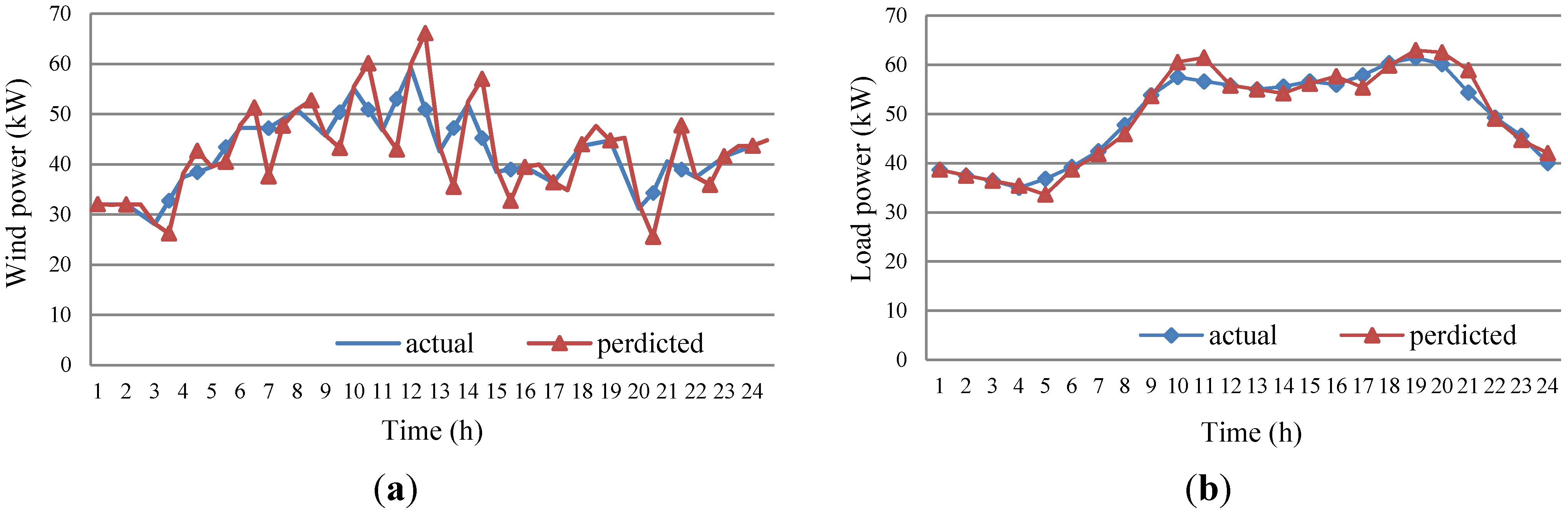
In combination with the known meteorological data, the above method can be adopted to figure out the predictive speed to finally deduce the wind power data, as shown in Figure 6a. This method can be also employed to work out the load power by dint of previous statistical data, as shown in Figure 6b. In the figure, blue represents the actual power, and red refers to the predictive power.
Figure 6 describes the predictive and actual value of wind and load power within 24 h. Upon calculation, the variation ratio and small error probability of the predictive wind power value are C = 0.4035, and P = 0.8085, respectively, and those of the predictive load power value are C = 0.2190 and P = 1, respectively. The two predictive evaluation indexes are consistent with requirements, which proves that the grey prediction method with residual modification can produce a satisfactory short-term prediction effect.
Figure 6. The predictive and actual wind and load power: (a) The predictive wind power curve within 24 h; (b) The predictive load power curve within 24 h.
Energies 08 01505 g006

3.3. Energy Coordinative Optimization Management Model of Microgrid System

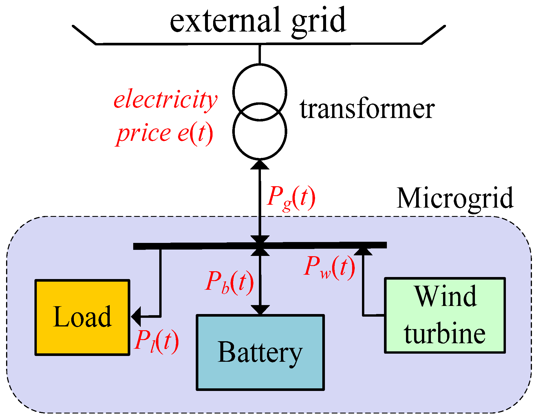
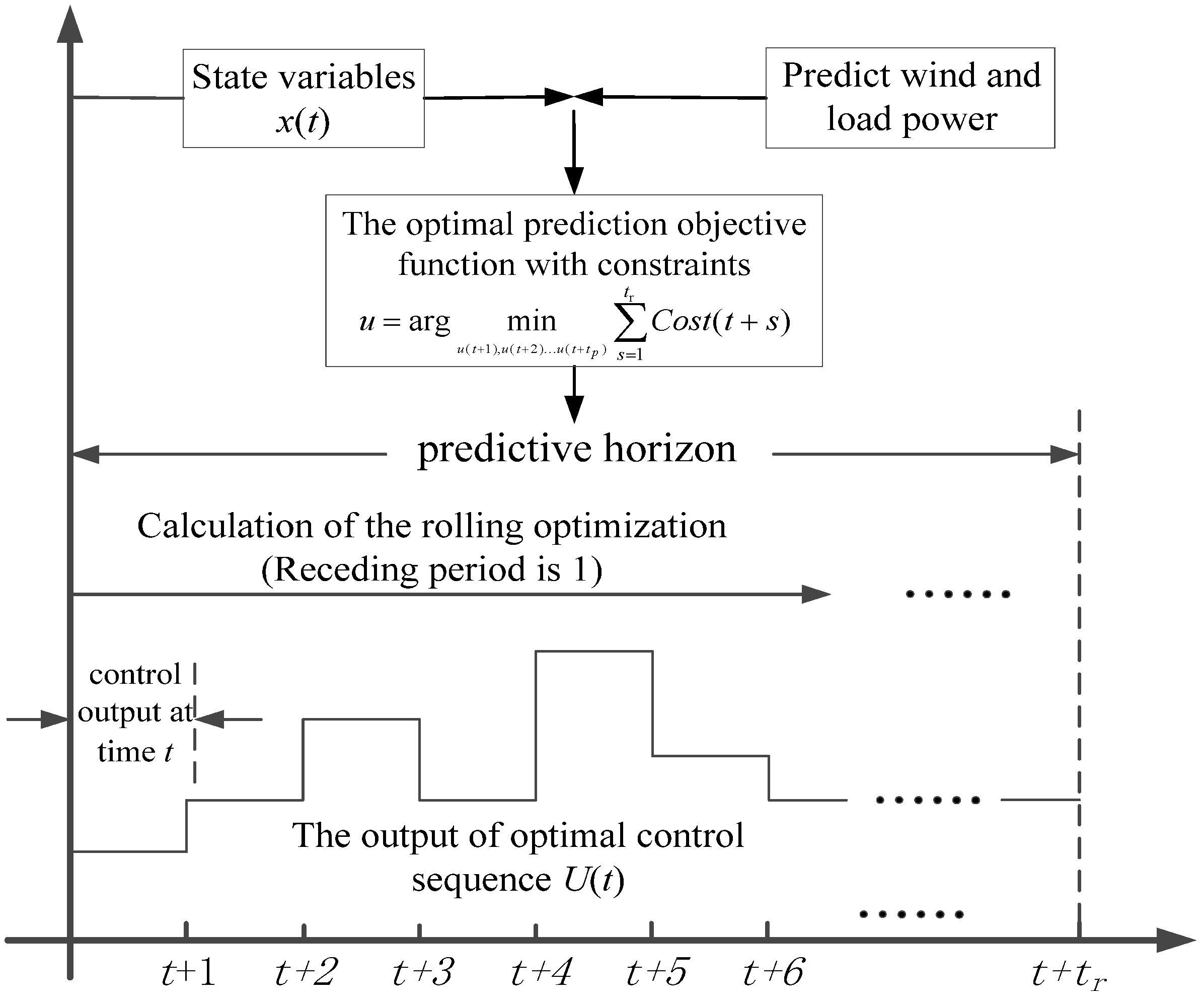
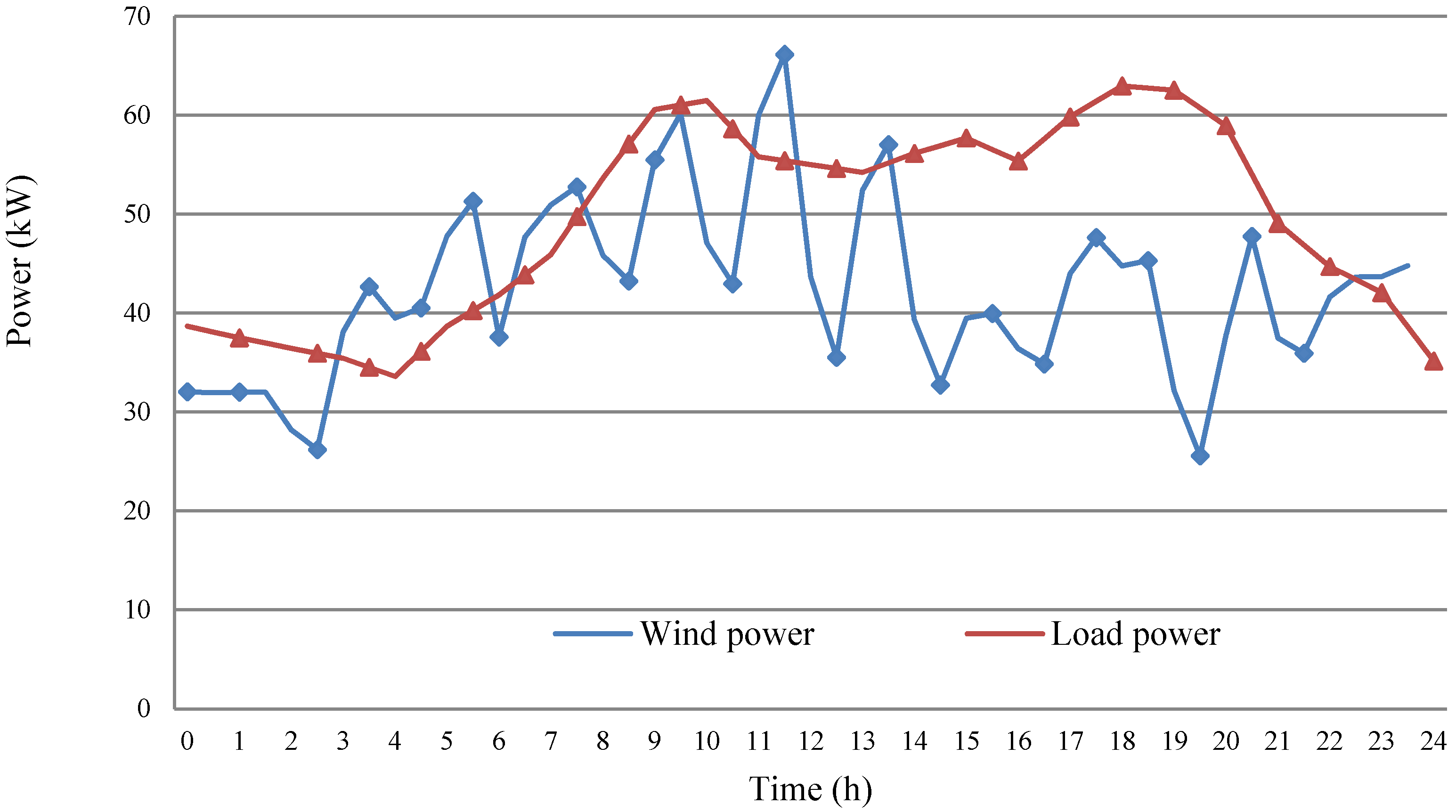
A microgrid energy coordinative optimization management system is supposed to plan and arrange the energy of wind turbines and storage batteries by dint of a reasonable and effective energy management strategy according to the short-term predictive power curve of wind and load a few days ago. In a given period, comprehensive consideration should be given to the predictive generating capacity of wind turbines, the remaining capacity of storage batteries, the power grid’s spot power price and load demand to build a model in which the objective function is to minimize the power consumption from the external grid and the constraints are constituted by the microgrid energy balance and the rated power of DGs. In this way, the capacity of power exchange between the microgrid and the external grid in each stage can be optimized to supply the electric energy accurately for the load at the lowest cost in real time.

3.3.1. Objective Function

Based on the guarantee of local load and power supply, the goal should be to minimize the consumption expenses from the external grid during the operation of the microgrid, which include the cost of the electricity purchased from the power grid, the earnings from selling electricity to the external grid, and the maintenance costs and depreciation losses of storage batteries:
min   C = t = 1 t r [ e S e l l ( t ) P g S e l l ( t ) + e B u y ( t ) P g B u y ( t ) + e b a t ( t ) P b a t ] Δ t
In the equation, eSell(t) refers to the spot power price when the electricity is sold to the external grid; eBuy(t) to the spot power price at which the electricity is bought from the external grid; ebat(t) to the management cost of storage batteries; PgBuy(t) to the electric power absorbed by the external grid (negative sign) at time t; PgSell(t) to the electric power generated by the external grid (positive sign) at time t; Pbat(t) to the active power of the storage batteries at time t; and Δt to the time interval of system operation (Δt = 1 h).

3.3.2. Constraints

(1) Power balance constraint:
P w ( t ) + P g ( t ) + P b ( t ) = P l ( t )
In the equation, Pw(t) refers to the power output of a wind turbine unit at the time t and Pl(t) to the power consumption at the time t. When positive values, Pg(t) and Pb(t) will represent the power output of external grid and storage battery at the time t, respectively; conversely, they will represent the power input.
(2) The constraints on the maximum power of the interaction between microgrid and external grid:
P g min P g ( t ) P g max
In the equation, Pgmin and Pgmax constitute the lower and upper limits of the power during the energy exchange between the microgrid system and the external grid.
(3) Constraints on the power output of storage batteries:
P b min P b ( t ) P b max
In the equation, Pbmin and Pbmax represent the minimum and maximum output power of the storage batteries, respectively.
(4) Energy balance constraints of the storage batteries:
E ( t + 1 ) = ( 1 τ ) E ( t ) P b ( t ) Δ t
where E(t) refers to the remaining capacity of a storage battery at time t and τ to the hourly self-discharge decay of a storage battery within a unit time (normally, τ = 10−4).
(5) Constraints on the charge and discharge rate of storage batteries:
Δ E min ( t ) Δ E ( t ) Δ E max ( t )
where △Emin(t) and △Emax(t) denote the minimum and maximum values of the charge and discharge rates.
(6) Constraints on the remaining capacity of the storage batteries
E min ( t ) E ( t ) E max ( t )
where Emin(t) and Emax(t) refer to the minimum and maximum values of storage battery capacity, respectively.

3.4. Energy Coordinative Optimization of Microgrid System Based on GA

A genetic algorithm (GA) is a self-adaptive probabilistic algorithm of global optimization that takes shape in the process of simulating heredity and evolution in natural environments [22]. Equipped with advantages such as excellent robustness, high efficiency, and parallelism, genetic algorithms are widely applied to combinational optimization [23].

3.4.1. The Objective Function of the Energy Coordinative Optimization of a Microgrid System

The objective function, which takes into account the cost of buying electricity from the power grid and the earnings from selling electricity to the power grid, is represented by Pg(t). If Pg(t) is positive, the external grid outputs power to the microgrid, on the other hand, if negative, the power flow reverses. The time step is denoted by s. The corresponding equation is Equation (29):
C G A = min s = 1 t r [ e S e l l ( t + s | t ) | P g ( t + s | t ) | + P g ( t + s | t ) 2 e B u y ( t + s | t ) | P g ( t + s | t ) | P g ( t + s | t ) 2 + e b a t ( t + s | t ) P b a t ( t + s | t ) ] Δ t
In the equation, the cost will be eSell(tPg(t) when Pg(t) is a positive value, but the cost will become −eBuy(tPg(t) when it is a negative value.

3.4.2. The RHC Optimization Based on a Genetic Algorithm

In this paper, the RHC optimization framework is employed, with the receding optimization range being tr and the receding step being 1 h. At time t, a solution for the optimization within the receding horizon [t t + tr] should be found, and the objective function should be minimized through calculating the optimal control sequence within receding horizon. In view of this, receding optimization range is added to Equation (29) to calculate the system operation cost during t and t + tr, which emerges in the following equation as a new objective function:
min s = 1 t r C ( t + s | t )
In the new objective function, the receding horizon not only takes account of the current situation, but also considers the system operation state at a future period of time. In this way, the optimization process will produce a better predictive dynamic control effect, with the basic flowchart of the algorithm shown in Figure 7.

3.5. Linearization of the Non-Linear Model in Energy Coordinative Optimization of Microgrid System

Mixed Integer Linear Programming (MILP) intends to optimize problems involving integer or discrete variables, and is widely applied due to its rapid computing speed and high accuracy. Considering that most of the problems that the actual system are constituted by non-linear problems and they are usually required to be converted into a linear expression if the MILP method is adopted, the key to finding a solution successfully is to linearize the non-linear problems effectively.
In the energy coordinative optimization management model, because the prices of selling and purchasing power are brought in, the energy exchange between external grid and microgrid has two input and output states. For this reason, a state variable α is introduced to represent the state of the energy flow between the external grid and microgrid. α = 0 indicates that the electricity is sold, and α = 1 indicates that the electricity is purchased, as expressed by Equation (31):
C M I L P = s = 1 t r [ e S e l l ( t + s | t ) P S e l l ( t + s | t ) α + e b a t ( t + s | t ) P b a t ( t + s | t ) + e B u y ( t + s | t ) P B u y ( t + s | t ) ( 1 α ) ] Δ t
The new constraints are added as follows:
{ P S e l l < N α P B uy < N ( 1 α )
As a proper margin, N is used to calculate in MILP. On this basis, the non-linear factors in the model can be transformed into a linear equation by the state variable α, and meanwhile, the optimization problem can be converted from a non-linear planning problem into a mixed integer linear planning problem, so MILP can be used to find a solution.
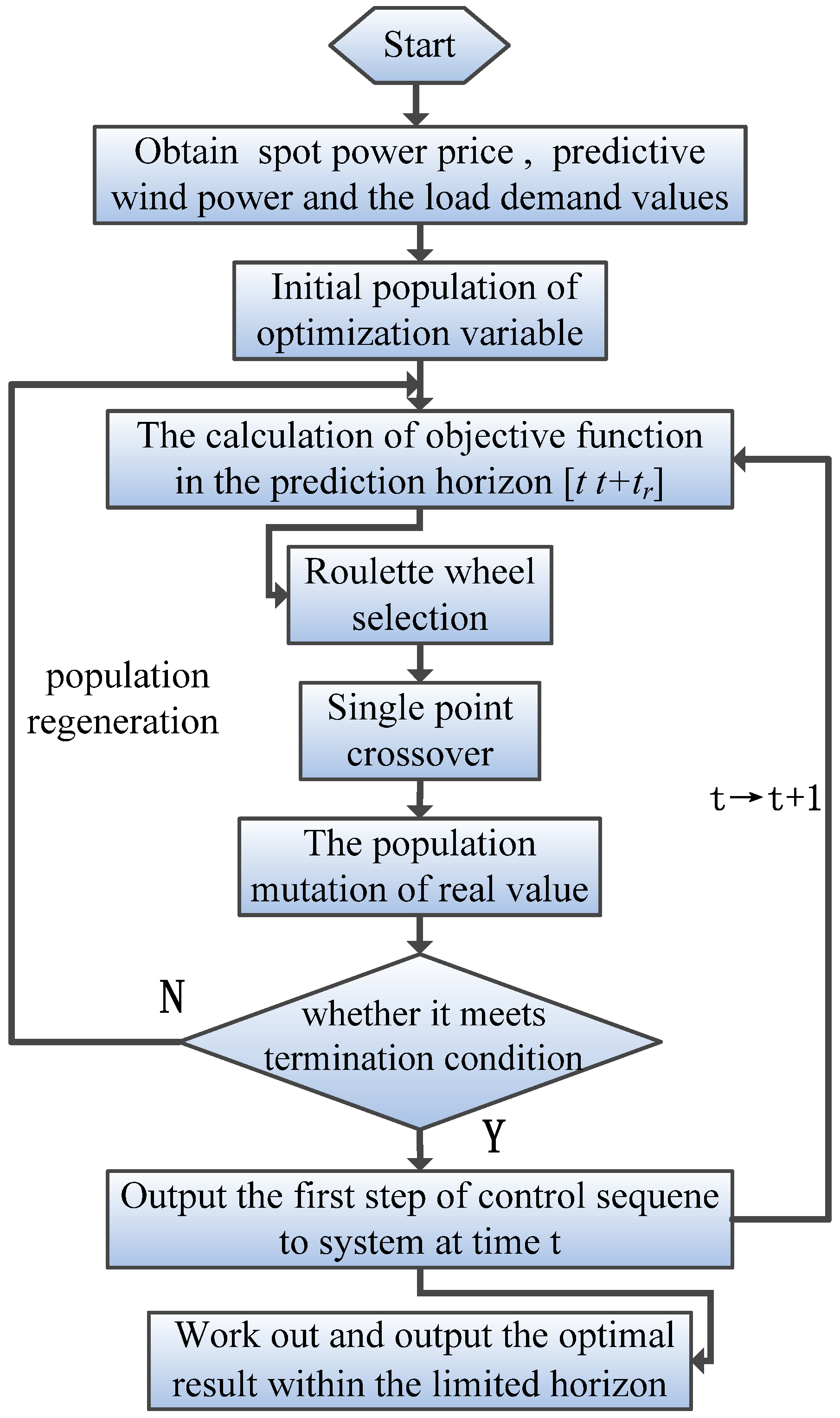
Figure 7. The flowchart of RHC optimization strategy based on GA.
Energies 08 01505 g007

3.6. The Specific Steps of a Microgrid System’s Energy Coordinative Optimization

The thinking of the receding optimization within limited horizon is applied. According to the description of the model and optimal control theory, specific steps are shown as follows. The energy coordinative optimization flowchart can be seen in Figure 8.
Step 1
Establish the microgrid model, including wind turbine model, storage battery model, spot power price model; initialization of the parameters involving the predictive wind power and the load demand values obtained in the predictive range and state variables Pw(t), Pg(t), Pb(t) and Pl(t).
Step 2
Establish the constrained objective function of economical optimization according to the actual demand by the microgrid’s energy coordinative optimization.
Step 3
Find a solution for the minimization problem within a limited horizon in the optimization range of [t t + tr]; in this step, every receding optimization will bring into existence a control sequence U(t) = {u(t|t),…,u(t + tr|t)}, whereby the solution for the control variable u(t|t) can be found at the first step in current moment; that is, Pg(t|t) at the first step constitutes the variables for the energy exchange between the external grid and microgrid and Pb(t|t) is the variable for the charge and discharge energy of the storage battery.
Step 4
The optimization horizon keeps receding: t = t + 1, return to Step 3.
Step 5
Output the optimal result within the limited horizon [t, t + tn] after the receding optimization stops.
Figure 8. Flowchart of energy coordinative optimization.
Energies 08 01505 g008

4. Experimental Results and Analysis

4.1. Main Parameters

In a microgrid’s economic schedule, a short-term schedule refers to an hourly schedule plan, which normally studies the output of DGs in 24 h. In this paper, a microgrid consisting of a wind turbine, storage battery and load is applied and the predictive output is decomposed into 24 time ranges based on one hour. In the optimization process, 0.0296 Yuan/kWh is taken as cost coefficient due to the addition of the storage battery unit. The main parameters of the model are shown in Table 4. Due to the use of a wind-storage-load microgrid model, the power selling price is subject to the on-grid price of wind power in the model. The 24-h spot power price is shown in Figure 9, where blue represents the purchasing price of power and red signifies the selling price of power.
Table 4. The output limitations of DGs.
NumberParameterPower Upper Limit (kW)Power Lower Limit (kW)
1Pg25−20
2Pb20−20
3E6020
4△E30−30
Figure 9. Spot power price curve in 24-h.
Energies 08 01505 g009
The 24-h wind and load power curves are predicted by the residual grey prediction method based on previous statistical data, as shown in Figure 10, where blue represents the predictive wind power curve and red signifies the predictive load power curve.
Figure 10. The prediction curve of 24 h.
Energies 08 01505 g010

4.2. The Inverter Control Optimization Result

In actual operation of a microgrid, not only will grid-connected operation emerge, but the islanded operation from the external power grid will happen. To verify that PQ control is able to control the DGs of the microgrid and stabilize system operation effectively in grid-connected operation mode, the experiment puts forward a design in which the given active power output of the storage battery declines from 20 to 15 kW at the time of 0.4 s and then rises to 20 kW at 1.2 s. Meanwhile, in the experimental design, the given active power output of the wind turbine rises from 21 to 22 kW at the time of 0.4 s and then to 26 kW at 0.6s, but afterwards, it declines to 25 kW at 1 s and to 22 kW at 1.2 s. Additionally, the given reactive output is 0 kVar. The experimental result is discussed below.
Figure 11a shows the changes of the active power of the storage battery and wind turbine in grid-connected operation mode; Figure 11b shows the changes of reactive power of the storage battery and wind turbine in grid-connected operation mode; and Figure 11c shows the changes of the effective values of phase voltage and line current output from the storage battery. According to these figures, the DGs are still able to provide stable voltage output when the value of given power changes. The current value varies sensitively as rapidly as power changing.
Figure 11. The effect of PQ control on a storage battery and wind turbine: (a) Active power of the storage battery and wind turbine; (b) Reactive power of the storage battery and wind turbine; (c) Effective values of phase voltage and line current output from the storage battery.
Energies 08 01505 g011aEnergies 08 01505 g011b
In islanded operation mode, V/f control is implemented over the storage battery in this experiment, where the active given output is set as 20 kW and the reactive power output as 0. The given active power of the wind turbine increases from 5 to 10 kW at the time of 0.5 s and becomes stable afterwards. The load grows from 15 to 20 kW at the time of 0.6 s and to 26 kW at 0.8 s, but afterwards, it returns to 20 kW at 1.2 s. The experimental result is discussed below:
Figure 12a focuses on the changes in active and reactive power output from the storage battery in off-grid mode and Figure 12b focuses on the changes in the voltage value, current value and frequency output from the storage battery. It can be seen that, with the changing load power, the voltage and frequency of the storage battery remain stable, and meanwhile, the current and power are able to change with the load power.
Figure 12. The effect of V/f control on the storage battery: (a) Active and reactive output power of the storage battery; (b) The phase voltage, line current and frequency output from the storage battery.
Energies 08 01505 g012aEnergies 08 01505 g012b

4.3. The Result Analysis of RHC Based on Prediction

After the predicted data of wind power and load power are figured out according to the proposed model, the intelligent GA is employed to find a solution for the objective function of economical optimization. The predictive step size is calculated from the first step and then accumulated step by step until the 10th step. After large quantities of tests, 100 initial populations are selected by means of the intelligent GA, with the largest number of iterations reaching 20,000, the mutation rate at 0.1 and the crossover rate at 0.8.
Figure 13a shows the optimization results of the external grid and battery power obtained by means of GA for different prediction lengths, and Figure 13b reveals the optimization result of the battery’s remaining capacity obtained by means of the GA for different prediction lengths. In these figures, red bars mean the charge and discharge capacity of the battery; blue bars signify the external grid power; and green bars refer to the battery’s SOC.
As shown by the experimental result, when the solution is found by means of the GA and the prediction length is 1, the microgrid will rely on the support of the external power grid; the storage battery will stop working; and the optimal control theory will be unable to optimize the result. As the prediction length increases, the optimization result will be smaller and the optimization will become increasingly obvious. When the prediction length is 5, the optimization results will converge. When the prediction length reaches 10, the optimization result will be nearly identical with that when the prediction length is 5. This suggests that a longer prediction length does not always produce a better optimization result.
Figure 13. The optimization result of a GA for different prediction lengths: (a) The optimization result of the external grid and battery power; (b) The optimization result of the battery’s SOC capacity.
Energies 08 01505 g013
Meanwhile, in order to verify the linear decomposition efficiency and accuracy of the non-linear model of a microgrid’s energy coordinative optimization, the MILP algorithm is used to find a solution.
Figure 14a,b is the optimization results of the external grid and battery power and battery’s remaining capacity, respectively, when the prediction length of MILP is 5. In these figures, red bars mean the charge and discharge capacity of the battery; blue bars signify the grid power; and green bars refer to the battery’s remaining capacity.
Figure 14. The optimization result when MILP’s prediction length is 5: (a) MILP’s receding optimization result of the grid and battery power; (b) MILP’s receding optimization result of the battery’s remaining capacity.
Energies 08 01505 g014
When the prediction length is 5, the optimization results of the two algorithms will converge and the change trends of the optimization curves are synchronized, which has manifested the accuracy of the RHC based on prediction strategy. According to the result, this linear method is able to figure out the energy direction of DGs in predictive horizon and satisfy the constraints of the charge and discharge capacity model of storage batteries. With the application of RHC based on prediction strategy, when the prediction length reaches a certain value if the constraints are satisfied, both GA and MILP could guarantee the economically optimal operation and the battery will not be charged or discharged frequently. Thus, it can be seen that this solution has taken account of not only economical optimization but also the service life of the storage battery.

4.4. The Comparison about Optimization Results of GA and MILP

To further verify that it is effective and feasible for the RHC based on prediction strategy to realize the energy coordinative optimization of microgrid, the performance of GA and MILP algorithms in the same microgrid model are compared in details in this section.
Table 5 shows the optimization result obtained after the global optimization of 24-h data without implementing RHC based on prediction strategy. The GA result is basically consistent with that of MILP, but GA achieves a more economical optimization result and takes full advantage.
Table 5. The comparison about the 24-h optimization results without implementing RHC based on prediction strategy.
NumberMethodOptimization Result
1GA45.6
2MILP48.49
As the receding optimization continues, not only the prediction length but also the computation time increases. However, as a result of the increasingly higher optimization accuracy, the final optimization result converges at a small range, as shown in Figure 15. Figure 15a demonstrates the RHC based on prediction results of GA and MILP, and Figure 15b shows the difference value curves of the based on prediction results of GA and MILP. In these figures, blue refers to the GA computation method; red to the MILP solution-finding method; and green to the difference values of the optimization results of GA and MILP.
Figure 15 has demonstrated that GA and MILP are respectively applied to finding a solution when the optimization method based on prediction is implemented. The optimization result reveals that the increase in receding predictive step can contribute remarkably to reduce the economic cost, and the optimization result will converge when the step size reaches a certain degree. When the step size is no less than 5, the MILP optimization result will converge as a constant value, but the GA optimization result will converge in a small range. Thus, it can be seen that a longer prediction length does not imply that the result is better. Though the computation time will increase with the step size, the optimization effect will not become better as the step size rises.
Figure 15. Comparison between the prediction-based results of different strategies: (a) The results of GA and MILP based on prediction; (b) The difference values of the prediction-based results of GA and MILP.
Energies 08 01505 g015
As shown in Table 6, the optimization result of GA is slightly superior to that of MILP, but their solutions are basically the same. With the complications of the microgrid model, it will be more difficult to linearize the non-linear objective function. Facing this problem, MILP will be unable to meet the computing requirements, but GA can be widely applied to finding a solution for non-linear optimization. Thus, it can be seen that the RHC based on prediction strategy has fully exploited the GA’s advantages; meanwhile, due to the satisfactory optimization effect, this strategy can optimize the energy flows between wind turbines, storage batteries, loads and external grids, and meet the requirements for the economical optimization of microgrid systems.
Table 6. The RHC of predictive optimal results for different strategies.
NumberMethodPrediction Length tr
12345678
1GA80.09376.09555.10750.62850.05350.08950.05550.054
2MILP80.09372.94954.33451.04450.14750.14750.14750.147
3Difference values03.1460.773−0.416−0.094−0.058−0.092−0.093

5. Conclusions

The energy coordinative optimization method not only is able to meet the actual demands of energy management strategy, but also guarantees reliably economic operation of microgrids, so it greatly contributes to the promotion and application of microgrids.
(1)
Based on the characteristics of microgrids, this paper proposes a method for energy coordinative optimization which focuses on the improvement of the economic benefits of microgrids in the prediction framework.
(2)
The generation power of wind turbines and load power are predicted through building a grey prediction model with residual modification, which has eliminated the unstable influence of wind power on energy optimization. Meanwhile, the data such as spot power price, wind power and predicted load power are applied in the optimization algorithm.
(3)
Comparing GA with MILP in finding the optimal solutions, MILP has higher computing speed, but non-linear computing become difficult after model becomes more complex. A GA can efficiently figure out the optimum solution in predictive horizon for the complex non-linear coordination control model of microgrids. The effectiveness and feasibility of the proposed method which integrates RHC and GA is verified by example.
(4)
As for future work, we think that energy coordinative optimization model of microgrids and various constraints such as economy, environment and maintenance cost need to be improved. Furthermore, the charge and discharge frequency of the storage battery and centralized, distributed and decentralized optimization algorithms need to be discussed.

Acknowledgments

This work was supported by the Science and Technology Project of the Beijing Municipal Commission of Education (PXM2014014212000061) and project of Collaborative Innovation Center of Electric Vehicles in Beijing.

Author Contributions

Changbin Hu designed the simulations and the study, Shanna Luo contributed to the theoretical analysis of microgrid systems and performed the economical optimization coordination control for microgrid systems. All authors have compared our new method with other method and approved the final manuscript.

Conflicts of Interest

The authors declare no conflict of interest.

References

  1. Lassetter, R.H.; Akhil, A.; Marnay, C. White Paper on Integration of Distributed Energy Resources. The CERTS Microgrid Concept; LBNL: Berkeley, CA, USA.
  2. Wang, R.; Li, K.; Zhang, C. Optimization allocation of microgrid capacity based on chaotic multi-objective genetic algorithm. Power Syst. Prot. Control 2011, 39, 16–22. [Google Scholar]
  3. Venkataramanan, G.; Marnay, C. A larger role for micro grids. IEEE Power Energy Mag. 2008, 6, 78–82. [Google Scholar] [CrossRef]
  4. Majumder, R.G.; Ledwich, A.G. Power management and power flow control with back-to-back converters in a utility connected microgrid. IEEE Trans. Power Syst. 2010, 25, 821–834. [Google Scholar] [CrossRef] [Green Version]
  5. Ai, X.; Cui, M.; Lei, Z. Environmental and economic dispatch of microgrid using chaotic ant swarm algorithms. J. North. China Electr. Power Univ. 2009, 36, 1–5. [Google Scholar]
  6. Zakariazadeh, A.; Jadid, S.; Siano, P. Smart microgrid energy and reserve scheduling with demand response using stochastic optimization. Int. J. Electr. Power Energy Syst. 2014, 63, 523–533. [Google Scholar] [CrossRef]
  7. Paiva, J.E.; Carvalho, A.S. Controllable hybrid power system based on renewable energy sources for modern electrical grids. Renew. Energy 2013, 53, 271–279. [Google Scholar] [CrossRef]
  8. Khalid, M.; Savkin, A.V. Minimization and control of battery energy storage for wind power smoothing: Aggregated, distributed and semi-distributed storage. Renew. Energy 2014, 64, 105–112. [Google Scholar] [CrossRef]
  9. Yucheng, H.; Xiaobo, D.; Zaijun, W. Hierarchical and distributed optimization of energy management for microgrid. Electr. Power Autom. Equip. 2014, 34, 154–161. [Google Scholar]
  10. Jun, X. Model Predictive Control for Energy Management of Microgrid. Master’s Thesis, East China University of Science and Technology, Shanghai, China, 2014. [Google Scholar]
  11. Ionela, P.; Enrico, Z. A model predictive control framework for reliable microgrid energy management. Electr. Power Energy Syst. 2014, 61, 399–409. [Google Scholar] [CrossRef]
  12. Chen, C.; Duan, S.; Cai, T. Microgrid energy management model based on improved genetic arithmetic. Trans. China Electr. Technol. Soc. 2013, 28, 196–201. [Google Scholar]
  13. Koyanagik, J.F.; Fujita, G.; Koyanagi, K.; Yokoyama, R. Field tests of a microgrid control system. In Proceedings of the 41st International Universities Power Engineering Conference, Newcastle, UK, 6–8 September 2006; pp. 232–236.
  14. Li, P.; Liu, Z.; Li, X.; Pan, Y. Modeling and simulation of microgrid based on synthesis control. High. Volt. Eng. 2011, 37, 2356–2362. [Google Scholar]
  15. Renhua, Y.; Wei, H.; Li, G. Structure and operation control of micro-grid. Adv. Power Syst. Hydroelectr. Eng. 2010, 26, 48–55. [Google Scholar]
  16. Zhang, Y. Study of Operation Optimization and Energy Management for Microgrid. Ph.D. Thesis, Hefei University of Technology, Hefei, China, 2011. [Google Scholar]
  17. Zhang, G.; Zhang, B. Wind speed and wind turbine output forecast based on combination method. Autom. Electr. Power Syst. 2009, 22, 109. [Google Scholar]
  18. Wang, L.; Singh, C. PSO-based multidisciplinary design of a hybrid power generation system with statistical models of wind speed and solar insolation. In Proceedings of the 2006 PEDES’06. International Conference on Power Electronics, Drives and Energy Systems, New Delhi, India, 12–15 December 2006; pp. 1–6.
  19. Wang, C. Analysis and Simulation Theory of Microgrid, 1st ed.; Science Press: Beijing, China, 2013; pp. 142–145. (In Chinese) [Google Scholar]
  20. Xie, K.; Song, Y. Optimal power flow based spot pricing algorithm via interior point methods—On the economic meanings of λp and λq. Autom. Electr. Power Syst. 1999, 2, 1000–1026. [Google Scholar]
  21. Muyeen, S.M. Wind Energy Conversion Systems, 1st ed.; Science Press: London, UK, 2012; pp. 197–226. [Google Scholar]
  22. Gabriel, L.; Enrique, A. Parallel Genetic Algorithms: Theory and Real World Applications,, 2nd ed.; Springer: Berlin, Germany, 2013; pp. 154–196. [Google Scholar]
  23. Renders, J.M.; Flasse, S.P. Hybrid method using genetic algorithms for global optimization. IEEE Trans. Syst. Man. Cybern. B Cybern. 1996, 26, 243–258. [Google Scholar] [CrossRef] [PubMed]

