A Parametric Energy Model for Energy Management of Long Belt Conveyors

Abstract

As electricity prices continue to rise, the increasing need for energy management requires better understanding of models for energy-consuming applications, such as conveyor belts. Conveyor belts are used in a wide range of industries, including power generation, mining and mineral processing. Conveyor technological advances are leading to increasingly long conveyor belts being commissioned. Thus, the energy consumption of each individual belt conveyor unit is becoming increasingly significant. This paper proposes a generic energy model for belt conveyors with long troughed belts. The model has a two-parameter power equation, and it uses a partial differential equation to capture the variable amount of material mass per unit length throughout the belt length. Verification results show that the power consumption calculations of the newly proposed simpler model are consistent with those of a known non-linear model with an error of less than 4%. The online parameter identification set-up of the model is proposed. Simulations indicate that the parameters can be identified successfully from data with up to 15% measurement noise. Results show that the proposed model gives better predictions of the power consumed and material delivered by a long conveyor belt than the steady-state models in the current literature.

1. Introduction

The rising electricity prices and changing tariff structures are driving an increasing need for efficient and cost-effective use of electricity, especially in energy-intensive industrial applications, such as bulk material transportation [1,2,3]. Electricity remains an important source of energy for industries. Large electricity consumers need an accurate understanding of their operations in order to take advantage of the increasing number of tariff structures being rolled-out [1,2]. The efficient and cost-effective running of belt conveyors, like any other application, requires accurate plant models to be used by optimizing algorithms, such as that demonstrated in [3]. This paper proposes a new energy model for belt conveyors (BCs) with long, troughed belts. This model is suitable for conveyors longer than 1 km. The ultimate goal is to use the proposed model for accurate assessment of the energy consumption and cost of operating long BCs.

Troughed conveyor belts are a widely-used method of bulk material transportation. They are used in power plants, mining and mineral processing, the food and chemical industry, as well as in ports [4,5]. The current technological trend sees increasingly longer belts being deployed, with lengths up to 20 km on a single flight [6,7]. A conveying system can also be further elongated in applications that connect several belts in series, so as to navigate a rough terrain [7]. However, long belts are more technically challenging to control at high speeds, and so, many are relatively slow with a typical speed of less than 8 m/s [8].

Energy efficiency in belt conveyors is achieved by matching belt speed to the input material feed rate in order to maximize the mass of material conveyed per unit length and, consequently, per unit of energy [9]. The mismatch between speed and the feed rate exists because, in practice, conveyors tend to operate at slightly below full capacity. BCs are usually oversized during design to cater to anticipated capacity expansions and sometimes to standardize component sizes in an effort to lower maintenance costs [10]. In mining applications, conveyors may be loaded by an excavator, resulting in an uneven loading of the belt, so that the overall material flow rate is 50%–70% of full capacity [11].

The majority of the current literature on belt conveyor modeling focuses on dynamic modeling of the belt tension, elastic properties of the belt material and modeling individual types of resistances [5,8,12]. However, there is also a need for the energy model to capture the quantities of material transferred by conveyors for the purposes of energy cost optimization, as demonstrated in [3]. The current models assume a steady-state condition with a uniform material mass per unit length through-out the whole belt [13,14]. On very long belts, the effect of variable mass per unit length can be significant, because it takes a significant amount of time for material to move from a loading point (at the tail) to a discharge point (at the head). The model proposed in this paper is able to accurately capture the amounts of material loaded on each section of the conveyor belt and, hence, to calculate an accurate value of power required by the conveyor.

The ISO 5048, DIN22101 and CEMA modeling standards provide a concise analytical model based on resistances, in particular the primary resistance [9,15,16,17]. The CEMA model requires knowledge of three friction coefficients, accounting for ambient temperature correction, belt-idler friction and belt-load flexure [16]. Unlike CEMA, ISO 5048 and DIN 22101 require only one primary friction coefficient and a more generic means of calculating other resistances [9,10,15]. As a result, they form the basis of the model proposed in this paper. However, all modeling standards are based on typical values of friction coefficients that require rules of thumb and an experienced engineer to estimate. A parametric model that can be estimated using field measurements therefore becomes a more useful and practical option for accurate predictions of energy consumption.

The proposed energy model uses a first-order partial differential equation (PDE) to capture the state of material on the belt and a two-parameter equation derived from established industry standards to quantify the conveyor’s power requirements. Unlike the previously proposed models, our model accounts for the different amounts of mass per length throughout the whole of the conveyor’s length, and it is therefore able to give a more accurate estimate of the belt’s energy consumption. The proposed model is verified by comparing its steady-state calculations to a model proposed by Zhang and Xia in [9]. The model in [9] is used for comparison, because it is also derived from ISO 5048. The results show that the proposed energy model gives power values close to those obtained from [9], under maximum loading conditions. A novel system identification set-up using a recursive algorithm to estimate the model parameter is proposed. The variables required for measurement on the proposed set-up are identified. A sensitivity analysis of the power equation is used to justify the different parameter convergence rates, and their practical implications are discussed. The proposed model is useful in applications when the conveyor speed is controlled, as shown in the case-study application. The case-study simulation of the proposed model is shown to perform better than the steady-state approach in scheduling of a CBS under a time-of-use tariff.

The remainder of the paper is organized as follows: Section 2 presents the derivations of the proposed model. Section 3 verifies the proposed model by comparing its BC power consumption calculations to those of an existing model. Section 4 investigates the accuracy of the proposed model’s calculations and presents a parameter identification procedure. Section 5 presents a simulation example illustrating the use of the proposed model on the day-ahead scheduling of a CBS. Section 6 presents the conclusions.

2. Conveyor Model

A troughed conveyor is powered by an electric motor-driven system and supported by a system of pulleys, as shown in Figure 1. The conveyor carries the bulk material on top of a troughed surface of a rubber belt. The troughed structure of the belt is maintained by sets of evenly-spaced idlers (see the cross-sectional view of Figure 1). Proper idler spacing is determined during the design phase as recommended by industry guidelines, such as [16,17], to avoid excessive belt sag and potential spillages. This ensures that the cross-sectional area of the belt is fairly constant. The belt is usually fitted with accessories, such as a feed chute at the tail end and a scraper below the head end.

Figure 1. Simplified sketch of a conveyor.

Figure 1. Simplified sketch of a conveyor.

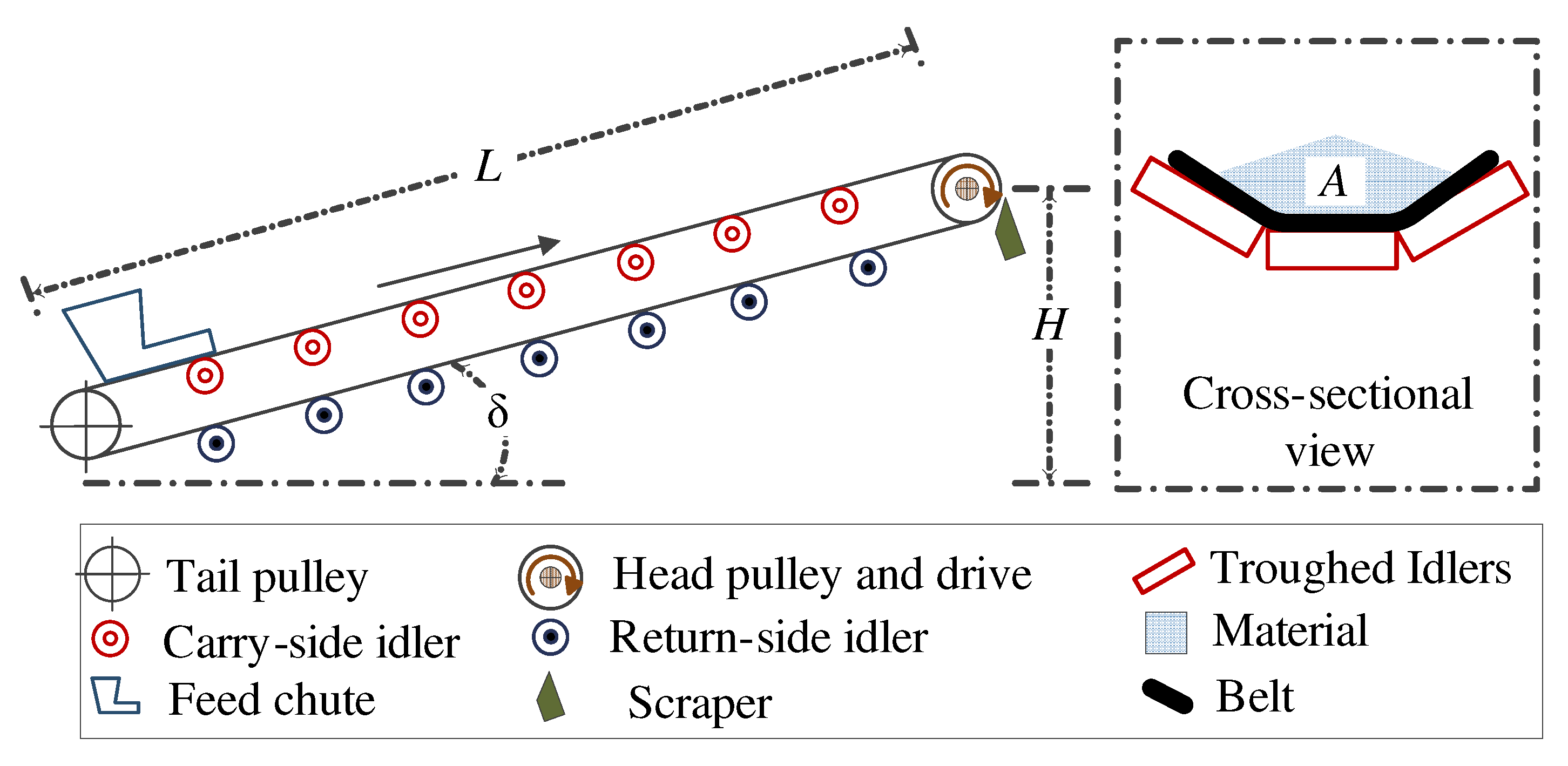
2.1. Conveyor Resistances

The electrical power required by a BC, P, is a product of the required peripheral driving force, $F_U$, the belt speed and drive system efficiency, η, i.e., $P=\frac{1}{\eta }{F}_U·v$ [9]. The peripheral driving force is given by,

$$F_U=F_H+F_N+F_{St}+F_S,$$

(1)

where $F_H$, $F_N$, $F_{St}$ and $F_S$ are the primary, secondary, slope and special resistances [15].

All resistances are dependent on the amount of material that the conveyor belt is carrying. By convention, this amount is specified in mass per unit length, $q(x,t)$. Thus, $q(x,t)$ is the mass of material per unit length of a conveyor belt section located at position x during time t in kg/m. Let:

$$\overline{q}\left(t\right)=\frac{1}{L}{\int }_0^{L}q(x,t)dt,$$

(2)

be the average mass per unit length over the total length, L, of the conveyor belt. When the flow of material on the BC is steady, $q(x,t)$ is uniform and constant. That is, $\overline{q}\left(t\right)=q(x,t)$ and $\overline{q}=\overline{q}\left(t\right)$.

In order to obtain an energy model based on amount of material, we begin by relating $\overline{q}$ to all of the resistances given in Equation (1).

2.1.1. Primary and Slope Resistances

Consider an L meters long belt with an artificial coefficient of friction f, inclined at an angle δ and operating under the Earth’s gravitational constant g. Suppose the unit mass per meter of the belt, carrying-side revolving idlers and return-side revolving idlers unit mass are $q_B$, $q_{RO}$ and $q_{RU}$, respectively. Then, the primary resistance is given by,

$$F_H=C_1+C_2·\overline{q},$$

(3)

where $C_1=fLg[q_{RU}+q_{RO}+2q_B\text{cos}\delta ]$ and $C_2=fLg\text{cos}\delta$.

$$F_{St}=C_7·\overline{q},\text{where}{C}_7=gH.$$

(4)

The slope resistance in Equation (4) is dependent on the height difference, H, between the tail and head ends of the conveyor. The slope and primary resistances account for the majority of the energy consumption, and they are easy to calculate [10]. For temperatures above 0 °C, the ISO and DIN standards prescribe a basic value of friction coefficient as 0.020 [17]. The exact value of f varies per installation, and a detailed account of its determination is given in [18]. For long conveyors, f is even lower than 0.016, a typical minimum value for short conveyors [10].

2.1.2. Special Resistance

Special resistance, $F_S$, depends on the special accessories fitted on the belt. Depending on the installation, the accessories may include; friction due to idler tilting, contact with skirt plates, contact with chute flaps and contact with discharge plows. $F_S$ is described by,

$$F_S=C_4·\overline{q}+C_5·{\overline{q}}^2+C_6,$$

(5)

where $C_4=c_{ϵ}{\mu }_0{L}_{ϵ}g\text{sin}ϵ\text{cos}\delta$ and $C_6={\mu }_0{L}_{ϵ}g\text{sin}ϵ\text{cos}\delta (c_{ϵ}+\text{cos}\lambda )q_B+A_{s}p{\mu }_3+B{K}_a$. Resistance from the material due to carry-side idler tilting is given by $C_4\overline{q}$. $C_4$ depends on the toughing factor $c_{ϵ}$, the length of the belt with tilted idlers $L_{ϵ}$ and ϵ idler tilt angle. $L_{ϵ}$ is equal to L minus the transition length at the tail and the head ends of the conveyor where the belt is guided towards/from a pulley. Usually, the transition length is small, and thus, $L\approxeq L_{ϵ}$ [17]. The resistance due to the return and carry-side idlers, scraper and contact with skit-plates is $C_6$. $C_6$ depends on the contact area of the scraper $A_s$, pressure applied by the scraper p, scraping factor $K_a$ and the toughing angle $\lambda$ as shown in Equation (5). $C_5={\mu }_{2}gl/\left(b_1^2\varrho \right)$ is the friction due to contact on the skirt plates [15]. $C_5$ depends on the skirt plate length l and width $b_1$ between the skirt plates. The skirt plates are installed over a very short length at the head of the conveyor, so as to guide material from the feeder and avoid spillages. Thus, $l\ll L$, and the effect of $C_5{\overline{q}}^2$ is local, independent of L and small compared with the overall resistance value [10]. $C_4$, $C_5$ and $C_6$ are equivalent to $k_1$, $k_2$ and $k_3$ of [9], respectively.

2.1.3. Secondary Resistance

Secondary resistance incorporates resistances occurring at the pulley, on the tail end due to acceleration of material and at the skirt plates due to acceleration of the material.

$$F_N=F_H(C_M-1).$$

(6)

ISO [15] indicates that for conveyors longer than 80 m, the secondary resistance is related to the primary resistance by a main resistance factor, $C_M$, as shown in Equation (6). For example, the values of $C_M$ for 100-m and 1 km-long conveyors are about 1.8 and 1.1, indicating that the secondary resistance is 44% and only 9% of $F_H$ for the two lengths, respectively. The approximation of $F_N$ suggested by Equation (6) shows that the contribution of $F_N$ on the total resistance is generally lower than 10% of $F_H$ when the belt length is 1 km or longer. For this reason, we consider belts of length 1 km or more as long BC and suitable for the model being proposed.

2.2. Modeling Energy Consumption

Substituting for the the secondary resistance and resistances from Equations (3) to (5) into Equation (1) leads to,

$$F_U=C_M{C}_1+C_6+(C_M{C}_2+C_4+C_7)·\overline{q}+C_5·{\overline{q}}^2.$$

(7)

Let the no-load and density parameters be ${\phi }_1=C_M{C}_1+C_6$ and ${\phi }_2=C_M{C}_2+C_4+C_7$, respectively. Due to the influence of $C_1$ and $C_2$, the values of parameters ${\phi }_1$ and ${\phi }_2$ increase quickly with increasing L. On the contrary, $C_5$ is independent of the belt length, and its value is much smaller than ${\phi }_1$ and ${\phi }_2$, since it is a component of $F_S$. As a result, $C_5$ is much smaller when compared with both ${\phi }_1$ and ${\phi }_2$, for long conveyors. Thus, for long conveyors, the total resistance is given by,

$$F_U={\phi }_1+{\phi }_2·\overline{q}+C_5·{\overline{q}}^2\approx {\phi }_1+{\phi }_2·\overline{q}.$$

(8)

For long conveyors, the approximation in Equation (8) is possible, because all of the non-linear components are from $F_S$, whose contribution is very small and, therefore, can be ignored. This means that for long belts, the total resistance can be approximated as linearly dependent on the average mass per unit length with a fair amount of accuracy. Moreover, $F_S$ does not occur in all conveyor belt installations. However, the power model in Equation (8) is generic and applies to all long conveyors, because the length-dependent coefficients of $F_S$ ($C_4$ and $C_6$) are incorporated into the parameters ${\phi }_1$ and ${\phi }_2$, so the presence or absence of $F_S$ would be easily accounted for by a parameter identification procedure.

For variable loading, $q(x,t)$ varies throughout the length of the belt. Therefore, according to Equations (2) and (8), the amount of power required to drive a long conveyor is,

$$P\left(t\right)=\frac{1}{\eta }({\phi }_1+\frac{{\phi }_2}{L}\underset{0}{\overset{L}{\int }}q(x,t)dx)·v\left(t\right).$$

(9)

Motor and drive mechanism efficiencies vary with changing motor speed and load [10]. However, variations become small for very large motors, such as those used to drive long conveyors. Thus, a constant value of η can be used, and the rest of the small efficiency variations will be incorporated within the modeling parameters. Equation (9) implies that calculating the energy consumption of a long conveyor requires the knowledge of only two parameters. Therefore, the energy consumed over a time interval [$t_1$, $t_2$] is given by,

$$E(t_1,t_2)=\frac{{\phi }_1}{\eta }\underset{t_1}{\overset{t_2}{\int }}v\left(t\right)dt+\frac{{\phi }_2}{\eta L}\underset{t_1}{\overset{t_2}{\int }}\left[{\int }_0^{L}q(x,t)dx\right]v\left(t\right)dt.$$

(10)

It is worth noting that relating the BC resistances to $\overline{q}$, in the derivation of Equation (8), introduces an error in power calculations when $q(x,t)$ varies. This error underestimates and overestimates the power requirement of different sections of the conveyor where $q(x,t)$ is higher and lower than $\overline{q}$, respectively. However, the overall error is reduced as the individual errors are summed in a long BC. Moreover, the impact of these errors becomes small for steep belts where $F_{St}$ is dominant.

2.3. Modeling Bulk Material Flow

The material mass per unit length is limited by the maximum carrying capacity of the belt, $q_{max}$. It can be understood from the cross-sectional view of the BC in Figure 1 that increasing $q(x,t)$ on a section of the belt would increase the height of material above the belt’s bottom surface until the material spills over when it can no-longer be contained by the troughing.

Figure 2 represents a longitudinal view of the material traveling at $v=3.3\overline{3}$ m/s on an 8-km conveyor belt, where the height of material above the bottom belt surface represents the magnitude of $q(x,t)$. Figure 2a shows the BC after $t_1=15$ min, just as the outlet of the chute is being stopped. Figure 2b shows the status of the same mass, M, of material on the belt after 39 min (i.e., at time $t_2+\delta t$). The bulk material on the conveyor flows from tail to head with negligible amount of diffusion. Therefore,

$$M=\underset{0}{\overset{p}{\int }}q(x,t)dx=\underset{v\delta t}{\overset{p+v\delta t}{\int }}q(x,t+\delta t)dx,$$

(11)

i.e., after 39 min, all of the mass of the material that was located before the position p or in the interval [0,3] km is now located within the interval [4.8, 7.8] km. This implies that material on the belt behaves like a wave traveling at a constant speed until it is spilled at the head of the conveyor. According to [19], this wave-like motion of material, where the mass balance Equation (11) holds, can be modeled using a one-dimensional transport equation. Thus, the motion of material on every segment of the conveyor’s length can be described by the partial differential equation (PDE) Equation (12) [19,20].

$$\frac{\partial }{\partial t}q(x,t)=-v\left(t\right)\frac{\partial }{\partial x}q(x,t),$$

(12)

where $v\left(t\right)$ is the belt speed. The total amount of material discharged by the conveyor, $M_{\text{out}}$, and the total amount of material entering the conveyor, $M_{\text{in}}$, during the time interval [$t_1$, $t_2$] are,

$$M_{\text{out}}=\underset{t_1}{\overset{t_2}{\int }}v\left(t\right)q(L,t)dt\text{and}{M}_{\text{in}}=\underset{t_1}{\overset{t_2}{\int }}v\left(t\right)q(0,t)dt=\underset{t_1}{\overset{t_2}{\int }}I\left(t\right)dt,$$

(13)

where L is the length of the conveyor and $I\left(t\right)$ is the input feed rate. For computational purposes, the model can be discretized using a finite difference method (FDM). FDMs offer a simple way of calculating numerical solutions of partial differential equations [21,22]. The model is discretized into $N_x$ samples in space and $N_t$ samples in time over a given total time period TD. The space sampling points are located at points $i·\Delta x$ (where $\Delta x=L/N_x$), and time sampling points occur at instances $n·\Delta t$ (where $\Delta t=\text{TD}/N_t$). Using the discretisation, the mass per unit length of material located at point $i·\Delta x$ on the belt during a time sample $n·\Delta t$ is denoted by $q(i,n)$, i.e.,

$$q(i,n)=q(i·▵x,n·▵t).$$

(14)

Figure 2. Wave-like property of material flow on the belt conveyor (BC). (a) time = t (15 min); (b) time = t + $\delta t$ (39 min).

Figure 2. Wave-like property of material flow on the belt conveyor (BC). (a) time = t (15 min); (b) time = t + $\delta t$ (39 min).

For brevity, the average and individual mass per length at different points at times $t=n·\Delta t$ are represented by ${\overline{q}}_n$ and ${\mathbf{q}}_n$, respectively. That is, ${\mathbf{q}}_n={\left[\begin{array}{ccc}q(1,n)& \dots & q(N_x,n)\end{array}\right]}^T$ and ${\overline{q}}_n$=${\sum }_{i=1}^{N_x}q(i,n)$. Usually, for scheduling, the modeling assumption is that both the input feed rate and belt speed are constant over a single time sample period, e.g., $v\left(t\right)=v_{n-1}\text{and}I\left(t\right)=I_{n-1},\text{for}t\in [(n-1)·\Delta t,n·\Delta t]$. It therefore follows that the discrete representation of the initial mass per length of material on the whole belt, $q(x,0)$, is ${\mathbf{q}}_0$. Using the above notation, the boundary conditions at the tail become,

$$q(0,n)=I_{n-1}/v_{n-1}.$$

(15)

The implicit backward Euler (BE) method is selected for solving Equation (12). This FDM method is unconditionally stable when solving the first order wave equation, such as Equation (12) [22]. The BE method uses a backward and a centered difference to approximate the time and space partial derivatives, respectively. A backward difference on the space derivative is used for the head of the conveyor, because $q(N_x+1,n)$ is invalid. Applying this method to Equation (12) results in the following $N_x$ equations,

$$q(i,n+1)=\left\{\begin{array}{ll}\begin{array}{c}2\{q(i-1,n)-q(i-1,n+1)\}/{\gamma }_i+q(i-2,n+1)\hfill \\ \{q(N_x,n)-q(N_x-1,n+1)\}/({\gamma }_i+1)\hfill \end{array}\hfill & \begin{array}{c}i=1,2,3,\dots N_x-1\hfill \\ i=N_x\hfill \end{array}\hfill \end{array}\right.,$$

(16)

where ${\gamma }_n=v_n\frac{▵t}{▵x}$. Equation (16) can also be represented in matrix and vector form as,

$$G_n{\mathbf{q}}_{n+1}=\{{\mathbf{q}}_n+{\mathbf{b}}_n·I_n/v_n\}\text{where}{G}_n\in {\mathcal{R}}^{N_x\times N_x}\text{,}{\mathbf{b}}_n\in {\mathcal{R}}^{N_x\times 1}.$$

(17)

The elements of the matrix $G_n$ and vector ${\mathbf{b}}_n$ are given by Equation (18).

$$G_n=\left[\begin{array}{ccccccc}1& {\gamma }_n/2& 0& \cdots & 0& 0& 0\\ -{\gamma }_n/2& 1& -{\gamma }_n/2& & 0& 0& 0\\ 0& -{\gamma }_n/2& 1& \ddots & 0& 0& 0\\ ⋮& & \ddots & \ddots & ⋮& ⋮& ⋮\\ 0& 0& 0& & 0& 0& 0\\ 0& 0& 0& & -{\gamma }_n/2& 1& {\gamma }_n/2\\ 0& 0& 0& & 0& -{\gamma }_n& (1+{\gamma }_n)\end{array}\right],{\mathbf{b}}_n=\left[\begin{array}{c}{\gamma }_n/2\\ 0\\ 0\\ 0\\ ⋮\\ 0\\ 0\end{array}\right].$$

(18)

3. Model Verification

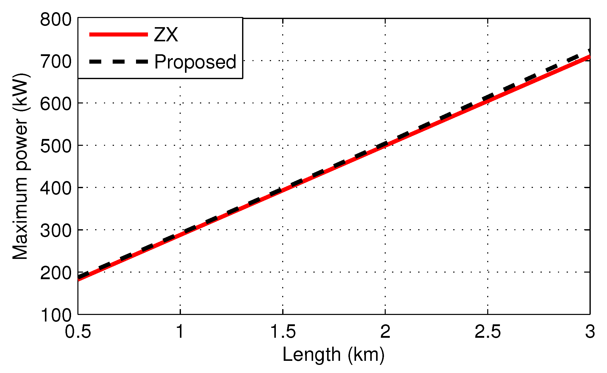
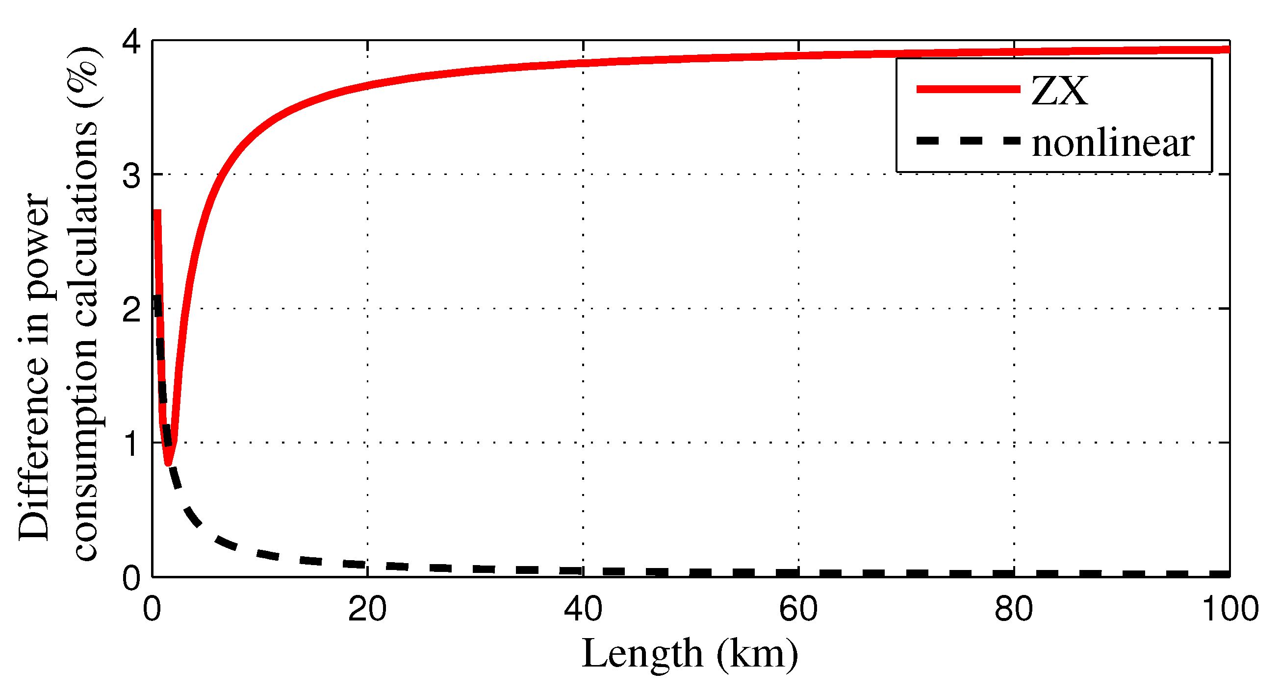
3.1. Steady-State Power Calculations

For verification, the 325 m-long conveyor example given in [23] is used, but with different lengths beginning from 500 m to 3 km in steps of 500 m. The maximum power required by the conveyor operating at full carrying capacity is calculated analytically, for both the proposed linear model of Equation (9) and the model from [9], labeled as ZX. Figure 3 shows that the maximum capacity power calculation values of the proposed linear model are close to those of ZX model for short and medium length conveyor belts.

The key assumption of the parametric power model in Equation (9) is that the non-linear components of the resistance are sufficiently small for long conveyors. The model in [9] and Equation (9) are both based on ISO 5048, even though Equation (9) is linear with two fewer parameters. In order to verify the linearity assumption, resistance values of each summation of Equation (8) are calculated, and their contribution to the total power consumption assessed, for two belts with lengths 500 m and 2 km.

Figure 3. Maximum capacity power calculations for both models.

Figure 3. Maximum capacity power calculations for both models.

Table 1 gives typical values of power and their percentage contribution to the total power when a belt given in [23] is operated at maximum speed and capacity. The calculations in Table 1 show that the non-linear component’s contribution is much smaller than that of the linear component. The effect of the non-linear component diminishes with increasing conveyor length, i.e., it decreases from 2.1% to 0.8% as the length is increased from 500 m to 2 km. Therefore, the linear simplification in Equation (8) is justified.

Table 1. Contributions of individual components to the total power required.

Unit	Component
	Total	${\phi }_1$	${\phi }_2·\overline{q}$	$C_5·{\overline{q}}^2$
L = 500 m
kW	191.3	41.7	145.7	3.9
%	100.0	21.8	76.1	2.1
L = 2 km
kW	508.1	123.7	380.4	3.9
%	100.0	74.9	24.3	0.8

Table 1. Contributions of individual components to the total power required.

Unit	Component
	Total	${\phi }_1$	${\phi }_2·\overline{q}$	$C_5·{\overline{q}}^2$
L = 500 m
kW	191.3	41.7	145.7	3.9
%	100.0	21.8	76.1	2.1
L = 2 km
kW	508.1	123.7	380.4	3.9
%	100.0	74.9	24.3	0.8

Figure 4 shows the percentage difference in maximum power calculations obtained by the linearized model compared to the proposed nonlinear model and the model of [9], for various lengths of the conveyor. The results show that the linearization error diminishes to 0% with increasing distance. The results also show that maximum power calculations from the proposed linear model deviate slightly from those of the model in [9], with an error that is generally less than 4%. Compared to the model in [9], the power calculation difference fluctuates for short distances below 2 km. The reason for this fluctuation is that the proposed model uses the DIN 22101 recommended values of $C_M$. These values are variable below 2 km, but a constant value of $C_M=1.05$ is used beyond the 2-km length.

Figure 4. Percentage differences in power consumption calculations for the ZX and non-linear models relative to the proposed model.

Figure 4. Percentage differences in power consumption calculations for the ZX and non-linear models relative to the proposed model.

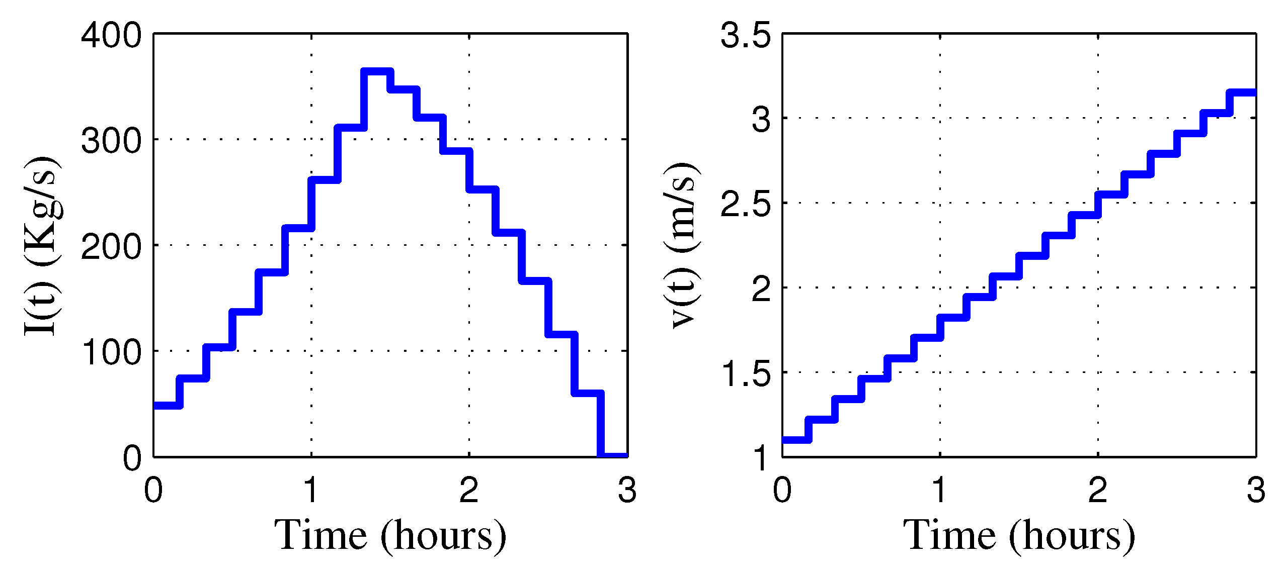
3.2. Variable Loading Calculations

The real advantage of the proposed PDE model, described by Equations (9) and (12), is its ability to capture the changes in the amount of material mass per unit length on the belt as the input feed rate and belt speed vary. The approach in [9] is that of a steady-state (SS) situation, where the belt loading resulting from the current input feed rate is assumed to instantaneously apply to the whole of the belt. An 8 km-long belt with the input feed rate and belt speed shown in Figure 5 is considered, in order to investigate the difference between the SS and PDE models.

The inputs in Figure 5 cover a duration of 3 h, and they vary every 10 min. The actual belt mass per length at the end of each sampling time can be calculated precisely because the inputs are known. This is possible because the conveyor belt effectively operates as a first-in-first-out (FIFO) queue of $q(0,t)$’s, whose lengths are obtained by multiplying their corresponding speeds by the 10 min sampling time (i.e., ${\tilde{L}}_n=v_{n-1}·\Delta t$). Figure 6 shows the positions of the different mass per lengths on the 8-km belt after 90 min when the inputs shown in Figure 5 are applied. For example, the mass per length at 4 km corresponds to the inputs $v=1.70$ m/s and $I=216$ kg/s applied 50 to 60 min after running the belt. Thus, $q(4\text{km},1.5\text{h})=216/1.70=127$ kg/m, as illustrated in Figure 6.

Figure 5. Input feed rate and belt speed.

Figure 5. Input feed rate and belt speed.

Figure 6. First-in-first-out (FIFO) queue model of the actual $q(x,t)$ on the belt after 1.5 h.

Figure 6. First-in-first-out (FIFO) queue model of the actual $q(x,t)$ on the belt after 1.5 h.

Figure 7 shows the simulation results of the proposed PDE model described by Equation (17) for the 8 km-long conveyor with inputs shown in Figure 5. The temporal and spatial resolutions used for the simulation are 5 min and 250 m, respectively. Figure 7 illustrates the wave-like flow of material on the belt described in Section 2.3. During simulation, the system of linear equations obtained from the model in Equation (17) is solved in the least-squares sense whenever the equality cannot be satisfied exactly. The good accuracy of the proposed flow model can be seen by comparing the actual $q(x,t)$ in Figure 6 to the data on the contour map of Figure 7 along $t=1.5$ h. For example, the contour map in Figure 7 shows that the $q(4\text{km},1.5\text{h})$ is just above 120 kg/s, $q(6\text{km},1.5\text{h})$ is in the range [80,100] kg/s and $q(8\text{km},1.5\text{h})$ is marginally above 40 kg/s. These simulated model values correspond closely to the actual values of $q(4\text{km},1.5\text{h})=127$ kg/s, $q(6\text{km},1.5\text{h})=93.7$ kg/s and $q(8\text{km},1.5\text{h})=44.1$ kg/s, shown in Figure 6.

Algorithm 1 implements the principle of the FIFO queue illustrated in Figure 6 to calculate the actual average mass per length on the belt, $\overline{q}\left(n\right)$. Algorithm 1 is also used to calculate the total amount of material received at the tail end of the conveyor after each sampling time n, ${\sum }_{i=1}^n{M}_{\text{out}}\left(i\right)$, given the initial uniform density of material on the belt ${\mathbf{q}}_0$. Algorithm 1 is based on the assumption that the belt is relatively flat and that there is an insignificant amount of material trampling backward or forward on the belt.

Figure 7. Three-dimensional view of $q(x,t)$ on the 8 km-long conveyor.

Figure 7. Three-dimensional view of $q(x,t)$ on the 8 km-long conveyor.

Figure 8 shows the power calculations at a 10-min sampling interval for the input shown in Figure 5. The proposed PDE model closely approximates the actual power requirement. The proposed PDE model performs better because it is able to estimate the $\overline{q}\left(n\right)$ with a small error compared to the SS approach. The proposed model’s calculated power values are on average 10.8% different from actual power. On the contrary, the SS model’s calculations give a very large difference with an average absolute percentage error of 40.4%.

The amount of material entering the conveyor over a time interval is easily calculated from the input feed rate using Equation (13), as $M_{\text{in}}\left(n\right)=I_n·▵t$. However, the material delivered at the head-end of the conveyor can only be estimated using a general formula. Equation (19) shows the three different estimates of $M_{\text{out}}$ using backward, forward and centered integrations of the conveyor model’s last node. Algorithm 1 can be used to verify the exact value of $M_{\text{out}}$.

$$\begin{array}{c}{M}_{\text{out}}\left(n\right)\approx △t·v_n·q(N_x,n)\text{(Bkd),}\hfill \\ M_{\text{out}}\left(n\right)\approx △t·v_n·q(N_x,n-1)\text{(Fwd),}\hfill \\ M_{\text{out}}\left(n\right)\approx △t·v_i·\frac{q(N_x,n)+q(N_x,n-1)}{2}\text{(Ctr).}\hfill \end{array}$$

(19)

Figure 8. Calculated (Algorithm 1) and modeled values of the conveyor’s power consumption.

Figure 8. Calculated (Algorithm 1) and modeled values of the conveyor’s power consumption.

Figure 9 shows the performance of each of the integration strategies, as well as the SS model when calculating the material delivered by the conveyor, over a period of 3 h. All of the methods from Equation (19) give close estimates of $M_{\text{out}}$, but the SS approach always over-estimates the amount of material delivered. However, the PDE model using a backward integration gives the closest final calculation of the material delivered, and it is therefore adopted for the rest of the paper. The SS model’s estimation is expected to improve with increasing belt speed, and the performance of all methods improves with the decreasing rate of variation in $I_n$ and $v_n$. Figure 10 shows that the mean percentage modeling error for calculating $M_{\text{out}}$ decreases with a decreasing ramp rate of $q(0,n)$. The results in Figure 10 show that the modeling error is below 10% for all integration methods when the ramp rate is below 1.2 kg/m/min. The accuracy of calculating $M_{\text{out}}$ can also be improved by decreasing the sampling time at the expense of degrading computational speed.

Figure 9. Calculated (Algorithm 1) and modeled amounts of material delivered by the conveyor after a given amount of time.

Figure 9. Calculated (Algorithm 1) and modeled amounts of material delivered by the conveyor after a given amount of time.

Figure 10. Effect of variation in $q(0,t)$ on the error when calculating $M_{\text{out}}$.

Figure 10. Effect of variation in $q(0,t)$ on the error when calculating $M_{\text{out}}$.

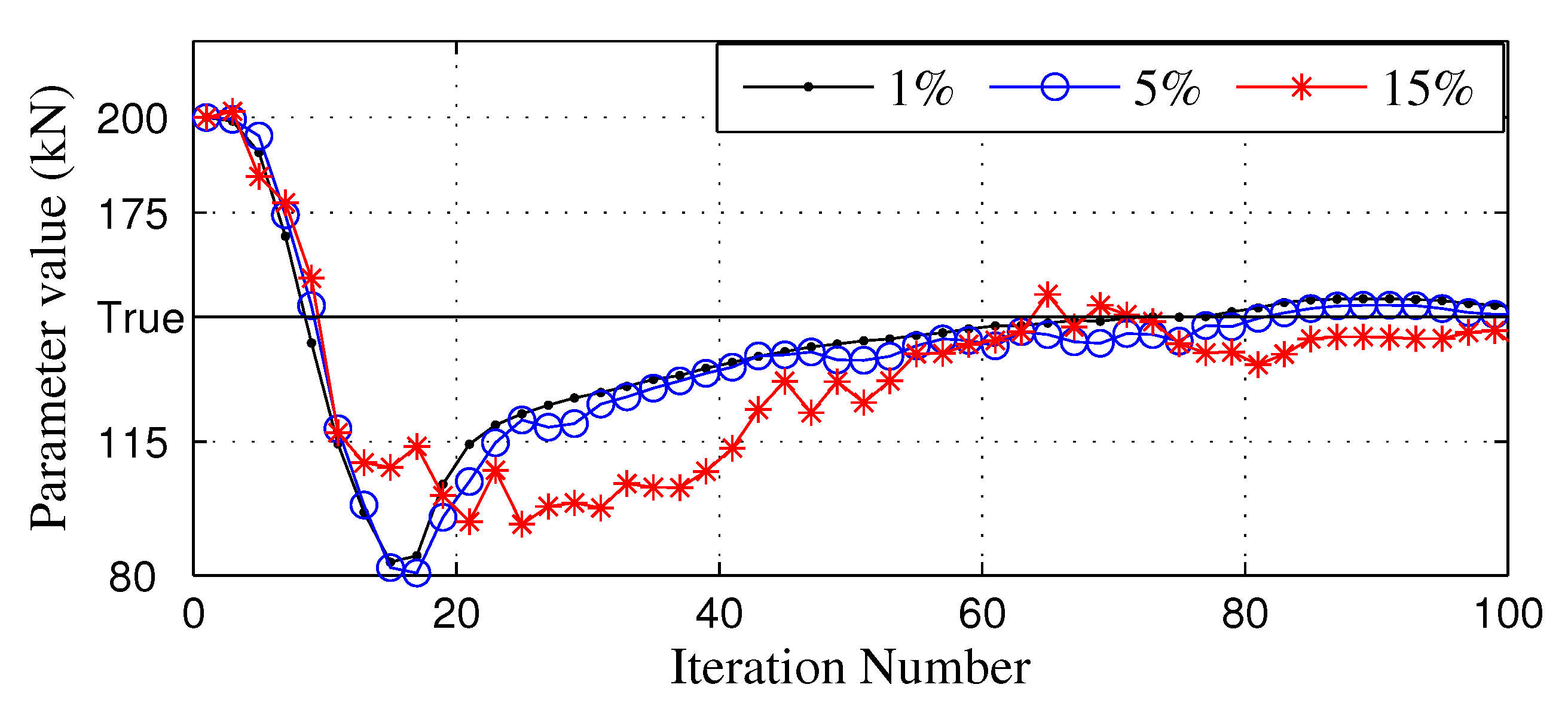
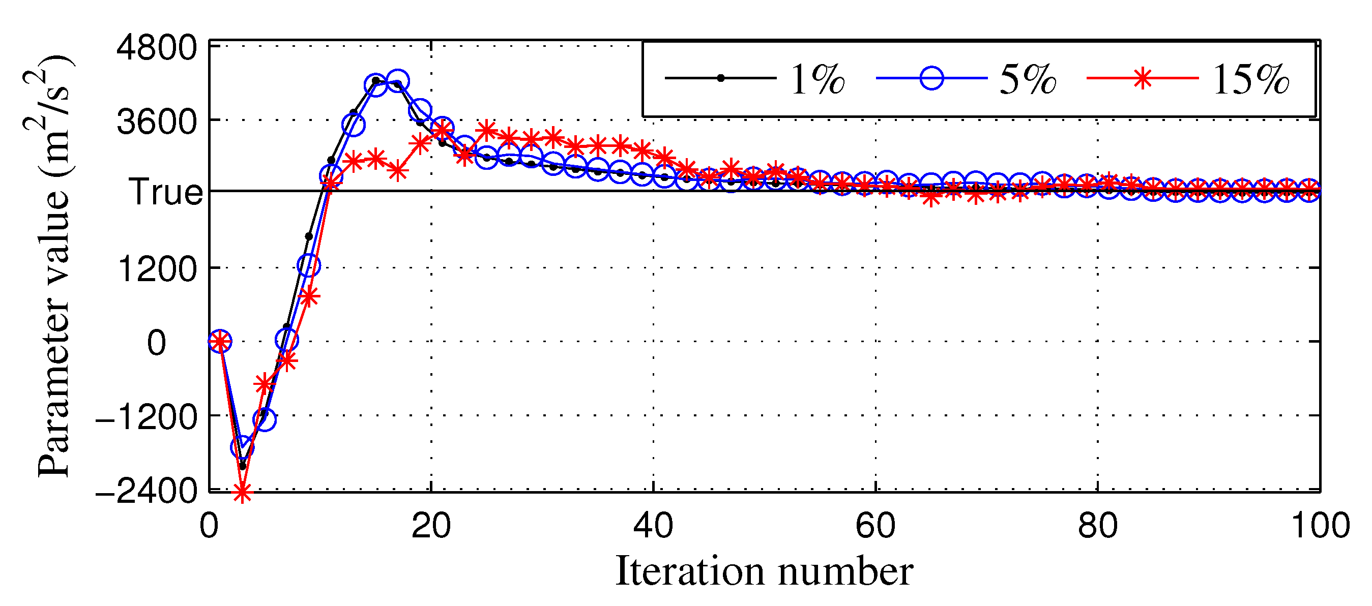
4. Parameter Identification

Figure 11 shows the set-up recommended for online estimation of the model parameters. This proposed online parameter identification requires the knowledge of three variables, namely: power consumption, belt speed and input feed rate. The feed rate, if not controlled, has to be measured at the tail-end of the conveyor. The purpose of Algorithm 1 is to keep track of the mass per unit length on the whole of the belt. The use of Algorithm 1 eliminates the expensive alternative of installing multiple sensors throughout the length of the belt. The identification process uses knowledge of the initial material distribution on the conveyor $q(x,0)$, continuous measurement and sampling of the feed rate and belt speed in order to estimate $q(x,t)$. It is important to note that $q(x,0)$ does not necessarily need to be measured. If it is unknown, any valid value, such as $q(x,0)=0$, can be used as an initial guess, and the Algorithm 1 would be able to reach an accurate estimate of $q(x,t)$ after some time when the effect of the guess has been eliminated. For example, it would take at most 30 min for the effect of the initial guess to be eliminated in a 2 km-long belt running at a minimum speed of 1.11 m/s.

Figure 11. Parameter identification set-up.

Figure 11. Parameter identification set-up.

Alternative to measuring $I\left(t\right)$ and $v\left(t\right)$, the mass per unit length at the tail-end of the conveyor, $q(0,t)$, can be measured. Due to an effectively constant cross-sectional area, the height of evenly-spread material above the belt provides a good estimate of $q(x,t)$, at any point x of the belt. However, there are even more accurate methods of measuring $q(x,t)$ using specialized belt weighing equipment or high-speed cameras and laser scanners coupled with advanced signal processing technologies [10,24].

The set-up in Figure 11 assumes that $I\left(t\right)$, $v\left(t\right)$, $M_{\text{out}}\left(t\right)$ and $P\left(t\right)$ can be measured from the BC. Algorithm 1 and the sequential parameter estimator (SPE) take synchronized samples of $v\left(t\right)$ and $I\left(t\right)$ as input to their calculations. The SPE uses the calculated mass per length ${\mathbf{q}}_n$, measured power output and input speed to approximate the belt energy model parameters.

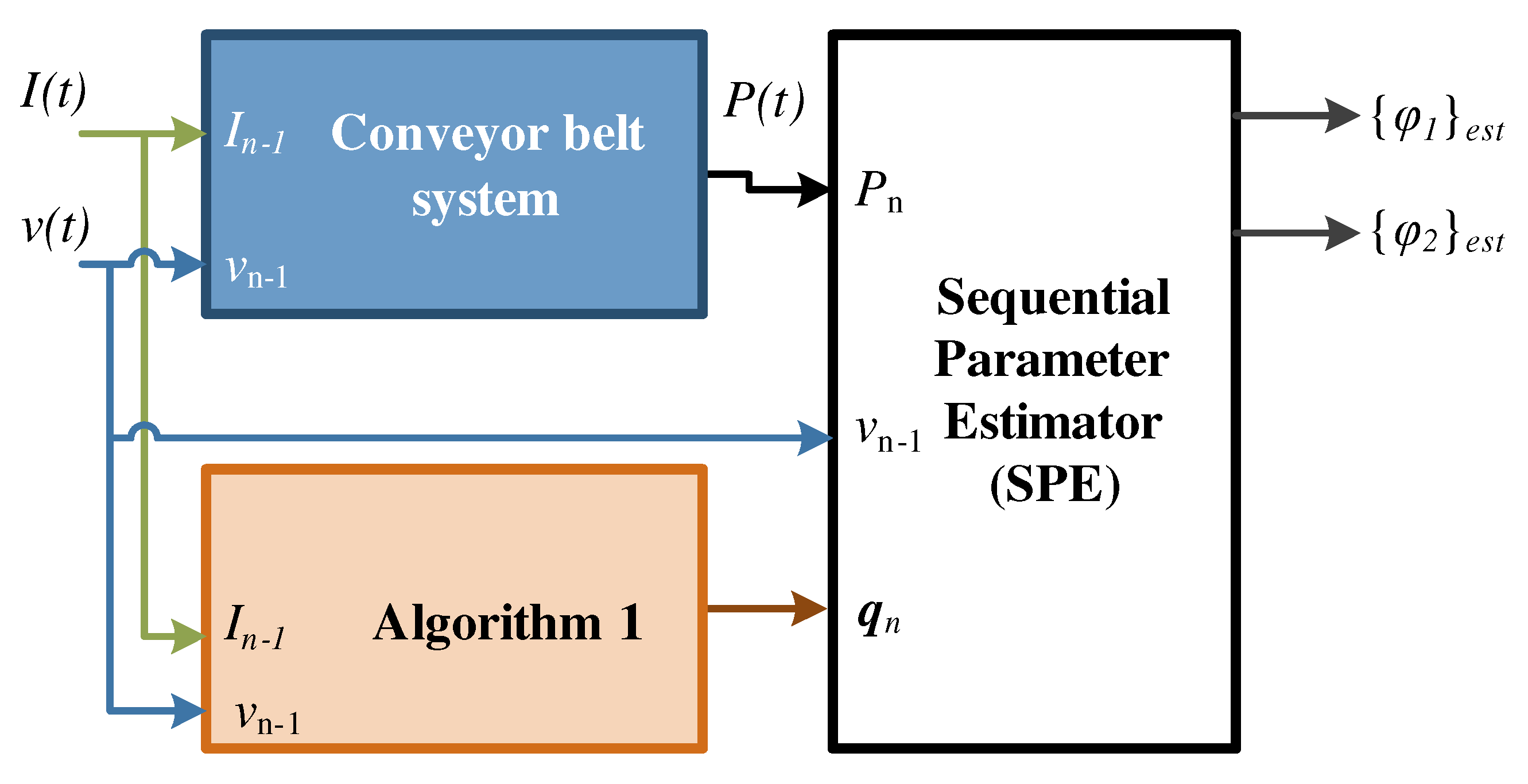
Parameter Estimation

The SPE algorithm recursively improves its estimated parameter values and their error covariance matrix by implementing a recursive least-squares algorithm, listed as Algorithm 2. Such an algorithm can be easily implemented into a hardware device to improve execution speed, as shown in [25]. At each time instance $t=n▵t$, the SPE uses the ${\mathbf{q}}_n$, as well as the measured belt speed and power output samples to calculate the current estimate of parameter values ${\left\{\phi \left(n\right)\right\}}_{\text{est}}={\left[\begin{array}{cc}\hfill {\left\{{\phi }_1\right\}}_{\text{est}}& {\left\{{\phi }_2\right\}}_{\text{est}}\hfill \end{array}\right]}^T$. The SPE uses the discrete version of the power Equation (9) $P_n={\mathbf{y}}_n^T·{\left\{\phi \left(n\right)\right\}}_{\text{est}}$, where ${\mathbf{y}}_n^T=\frac{1}{\eta }·{\left[\begin{array}{cc}\hfill v(n-1)& v(n-1)\overline{q}\left(n\right)\hfill \end{array}\right]}^T$.

In practice, the measurement of variables required for parameter estimation is likely to contain noise. Figure 12 and Figure 13 show the effect of measurement noise on the estimation of parameters. This simulation considers a belt with specifications similar to those found in [13], so that the true parameter values are ${\phi }_1=147.72$ kN and ${\phi }_2=2445.5$ m${}^2$/s${}^2$. The true value of a parameter is labeled as “true” on the y-axis. The results are shown for simulations with varying sizes of percentage noise errors. The measurements used are sampled at 10-min intervals, while the inputs are varied as shown in Figure 5. Figure 12 and Figure 13 show that the SPE algorithm takes longer to converge as the magnitude of noise increases. Thus, using precise measurement instruments will result in quicker estimation of the energy model parameters.

Figure 12. Convergence of the no-load parameter, ${\phi }_1$, for different measurement noise levels.

Figure 12. Convergence of the no-load parameter, ${\phi }_1$, for different measurement noise levels.

Figure 13. Convergence of the density parameter, ${\phi }_2$, for different measurement noise levels.

Figure 13. Convergence of the density parameter, ${\phi }_2$, for different measurement noise levels.

A comparison between Figure 12 and Figure 13 shows that the estimation of ${\phi }_2$ converges to its true value faster than that of ${\phi }_1$. The rate of convergence in parameter estimation is related to its the sensitivity to the output [26]. Since the state equation is independent of the parameters, the parameter output sensitivities, $S_{{\phi }_1}^P$and $S_{{\phi }_2}^P$, are given by,

$$\begin{array}{cc}{S}_{{\phi }_1}^P=dP/d{\phi }_1\hfill & =v(n-1),\hfill \\ S_{{\phi }_2}^P=dP/d{\phi }_2\hfill & =v(n-1)·\sum _{i=0}^{N_x}q(i,n)/N_x.\hfill \end{array}$$

(20)

In a typical operation, the average mass per unit length of a conveyor is a large value, bigger than about 50% of the belt’s $q_{\text{max}}$, and so, usually, ${\sum }_{i=0}^{N_x}q(i,n)/N_x\gg 1$ kg/m [11]. Therefore, generally, the power used by the conveyor is more sensitive to ${\phi }_2$ than ${\phi }_1$, i.e., $S_{{\phi }_1}^P<S_{{\phi }_2}^P$. This explains the different convergence rates shown in Figure 12 and Figure 13. Therefore, for this model, it is easier to identify the true value of ${\phi }_2$ than that of ${\phi }_1$. This implies that, in practice, the time it takes to get convergence of ${\phi }_1$ will determine the duration of a successful identification exercise.

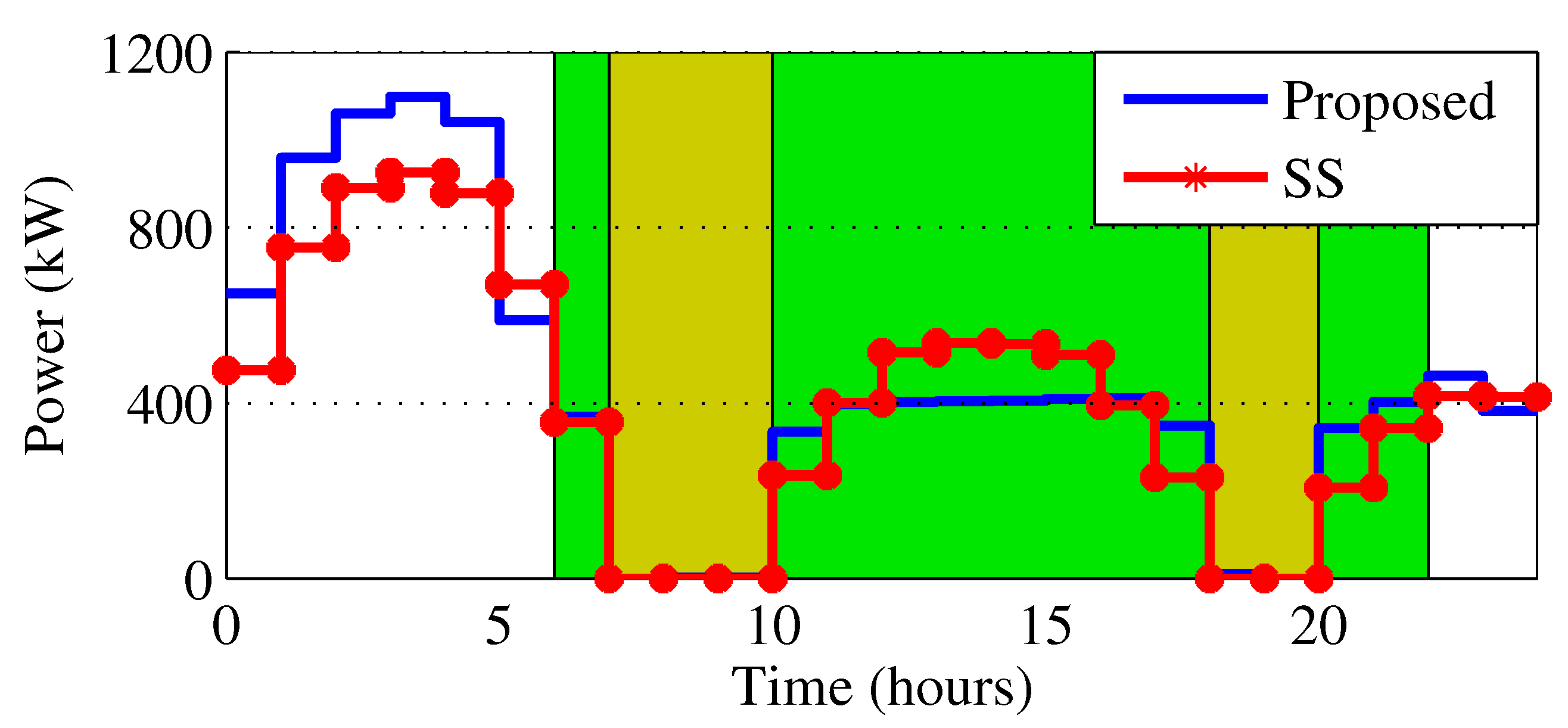
5. Application Case-Study

Consider the day-ahead optimal scheduling of the an 8 km-long coal conveying belt transporting coal from a stockyard to storage silos feeding the boilers of a power plant, explained in [1]. Assuming that the belt is initially empty (i.e., ${\mathbf{q}}_0={[00\cdots 0]}^T$) and operating under Eskom’s RuralFlex, the time-of-use (TOU) electricity tariff is given by Equation (21) [27]. The objective of the schedule is to find an energy-cost effective way of replenishing the silos as the power plant consumes the coal. Thus, the coal conveying process is restricted to maintaining the amount of coal in the silos between the lower $S{T}_L$ and upper $S{T}_U$ storage limits of 1958 and 4756 tons, respectively. The silos initially have $S{T}_0=2460$ tons of coal. The electricity load supplied by the power station determines the rate at which the coal is being consumed from the silos [1].

$${\pi }_n=\left\{\begin{array}{cc}\begin{array}{c}0.44\text{R/kwh,}\text{off-peak}n\in [1-6,23-24]\hfill \\ 3.27\text{R/kwh,}\text{peak}n\in [7,11-18,21-22]\hfill \\ 0.84\text{R/kwh,}\text{standard}n\in [8-10,19-20]\hfill \end{array}\hfill & .\hfill \end{array}\right.$$

(21)

The optimal schedule has to optimize the energy and mechanical costs, while meeting the hourly coal demand ($D_n$) and operating within storage ($S{T}_L,S{T}_U$), belt capacity ($q_{\text{max}}$) and actuator limits ($I_{\text{max}},v_{\text{max}}$). The SS approach scheduling optimization is given by Equation (22).

$$\begin{array}{c}{\mathbf{\text{min}}}_{\{v_n,I_n\}}\sum _{n=1}^{N_t}P\left(n\right)·{\pi }_n+\varpi \sum _{n=2}^{N_t}(v_n-v_{n-1})\\ \mathbf{\text{s.t}}\\ S{T}_L\le S{T}_n=S{T}_{n-1}+▵t·I_n-\frac{▵t}{3600}·D_n\le S{T}_U,\\ v_n\in [0,v_{\text{max}}],I_n\in [0,I_{\text{max}}],{\overline{q}}_n\in [0,q_{\text{max}}],\\ \text{Given}S{T}_0,\\ \text{where}{\overline{q}}_n=I_n/v_n\text{and}P\left(n\right)=\frac{1}{\eta }({\phi }_1+{\phi }_2·{\overline{q}}_n)·v_n,\forall n\in [0,N_t]\end{array}$$

(22)

The biggest source of error for the SS approach in conveyor belt optimal scheduling comes from its failure to account for the transition time from the initial condition where the belt’s $q(x,t)$ may be less than ($q_{\text{max}}$). It has already been illustrated in Section 3.2 that this may lead to miscalculations of the power usage and the amount of material delivered. An alternative is to use the proposed model as shown in Equation (23). The added accuracy of the proposed model comes with an added computational cost, since more variables have to be added to the optimization problem. This is because the proposed model discretizes the conveyor in both space and time, while the SS approach only involves time discretisation. The optimization problem Equation (23) is solved using active set methods solver implemented in MATLAB. The optimization of Equation (23) converges quickly when a feasible sub-optimal starting point is provided. This initial starting point can be easily generated by simulating the belt first with inputs that obey the storage bound constraints.

$$\begin{array}{c}{\mathbf{\text{min}}}_{\{v_n,I_n,{\mathbf{q}}_n\}}\sum _{n=1}^{N_t}P\left(n\right)·{\pi }_n+\varpi \sum _{n=2}^{N_t}(v_n-v_{n-1})\\ \mathbf{\text{s.t}}\\ G_n·{\mathbf{q}}_{n+1}={\mathbf{q}}_n+{\mathbf{b}}_n·q(0,n),\\ S{T}_L\le S{T}_n=S{T}_{n-1}+v_n·q(N_x,n-1)-\frac{▵t}{3600}·D_n\le S{T}_U,\\ v_n\in [0,v_{\text{max}}],I_n\in [0,I_{\text{max}}],q(i,n)\in [0,q_{\text{max}}],\\ \text{Given}{\mathbf{q}}_0\text{and}{S}_0,\\ \text{where}P\left(n\right)=\frac{1}{\eta }{\phi }_1{v}_n+\frac{1}{\eta L}{\phi }_2{v}_n\sum _{i=1}^{N_x}q(i,n),\\ {\gamma }_n=v_n\frac{\Delta t}{\Delta x}\text{and}q(0,n)=I_{n-1}/v_{n-1},\\ \forall n\in [0,N_t],\text{and}\forall i\in [0,N_x]\end{array}$$

(23)

The optimal day-ahead schedules of both the SS approach and PDE model are shown in Figure 14. The background colors of Figure 14 correspond to the different TOU tariff rates given in Equation (21). The proposed model estimates that the BC consumes 10.49 MWh, while the SS approach gives 9.69 MWh, and the resulting energy cost calculations of the proposed model are 6.4% higher. In Figure 14, the prominent difference between the two schedules occurs during the first 5 h of the day, where the PDE schedule requires more power than the SS model. The difference is caused by the fact that the SS model assumes that the conveyor begins delivering material into the storage from the first second. This is, however, not true, since the belt is initially empty, and so, coal has to travel from the loading point to the tail end, which is 8 km away. Thus, the SS approach wrongly underestimates the energy consumption and cost of the BC’s operation.

Both solutions obtained from solving Equations (22) and (23) are feasible. That is, both solutions predict that $S{T}_L\le S{T}_n\le S{T}_U,\forall n\in [0,N_t]$. However, simulating the optimization solutions with the PDE flow model of Equation (12) illustrates that the SS approach’s solution violates the storage bounds, as shown in Figure 15. The results in Figure 15 show that the level of storage predicted by the proposed model is relatively accurate. However, the SS approach creates a schedule that actually violates the storage bound constraints.

Figure 14. Power consumption of optimized schedules.

Figure 14. Power consumption of optimized schedules.

Figure 15. Predicted (pred) and flow model simulated (sim) storage level for both optimization solutions of Equations (22) and (23).

Figure 15. Predicted (pred) and flow model simulated (sim) storage level for both optimization solutions of Equations (22) and (23).

6. Conclusions

This paper has proposed an energy model with two parameters based on the belt resistances, for long belt conveyors with troughed belts. The model uses a partial differential equation to capture the varying amounts of mass per unit length on the belt in order to give a more accurate representation of the transported bulk material. The proposed model provides steady-state power calculations that are close to models found in the current literature. The proposed model is shown to estimate power usage of a long conveyor belt more accurately than the existing steady-state power models. The proposed model’s ability to accurately account for the amount of material being transferred by the conveyor makes it more useful in practice than the steady-state models currently available in literature. An online identification set-up for estimating the true values of the model’s parameters is proposed and simulated for an 8 km-long conveyor. The identification results show that precise measuring equipment is required for speedy identification and that it is easier to estimate the true value of the model density parameter than that of the no-load parameter. The proposed model is applied in a case-study application simulation to demonstrate its superiority over the steady-state approach. Simulations show that, unlike the SS approach, the proposed model is able to provide a schedule that does not violate storage level constraints.

Future work on the model shall consider calculating the power requirement of the BC by summing the resistances of shorter sections of the conveyor’s length. This approach is likely to improve the calculation of the primary and secondary resistances’ contributions to the overall power requirement of BCs.

References

1. Mathaba, T.; Xia, X.; Zhang, J. Analysing the economic benefit of electricity price forecast in industrial load scheduling. Electr. Pow. Syst. Res. 2014, 116, 158–165. [Google Scholar] [CrossRef]
2. Granell, R.; Axon, C.J.; Wallom, D.C.H. Predicting winning and losing businesses when changing electricity tariffs. Appl. Energy 2014, 133, 298–307. [Google Scholar] [CrossRef]
3. Mathaba, T.; Xia, X.; Zhang, J. Optimal scheduling of conveyor belt systems under critical peak pricing. In Proceedings of the International Power and Energy Conference (IPEC) 2012, Ho Chi Minh City, Vietnam, 12–14 December 2012; pp. 315–320.
4. Fedorko, G.; Molnar, V.; Marasova, D.; Grincova, A.; Dovica, M.; Zivcak, J.; Toth, T.; Husakova, N. Failure analysis of belt conveyor damage caused by the falling material. Part I: Experimental measurements and regression models. Eng. Fail Anal. 2014, 36, 30–38. [Google Scholar] [CrossRef]
5. Wheeler, C.A.; Roberts, A.W.; Jones, M.G. Calculating the Flexure Resistance of Bulk Solids Transported on Belt Conveyors. Part. Part. Syst. Charact. 2004, 21, 340–347. [Google Scholar] [CrossRef]
6. Zamorano, S. Main Article Belt Conveyor Technology Long Distance Conveying—Choosing the Right Option; Bulk Solids Handling: Houston, TX, USA, 2011. [Google Scholar]
7. Ristić, L.B.; Jeftenić, B.I. Implementation of fuzzy control to improve energy efficiency of variable speed buk materail transportation. IEEE Trans. Ind. Electron. 2012, 59, 2959–2968. [Google Scholar] [CrossRef]
8. Lodewijks, G. The design of high speed belt conveyors. In Proceedings of the Conference on Belt Conveying-BELTCON 10, Midrand, South Africa, 19–21 October 1999.
9. Zhang, S.; Xia, X. Modeling and energy efficiency optimization of belt conveyors. Appl. Energy 2011, 88, 3061–3071. [Google Scholar] [CrossRef]
10. Hiltermann, J.; Lodewijks, G.; Schott, D.L.; Rijsenbrij, J.C.; Dekkers, J.A.J.M.; Pang, Y. A methodology to predict power saving of troughed belt conveyors by speed control. Particul. Sci. Technol. 2011, 29, 14–27. [Google Scholar] [CrossRef]
11. Jeftenić, B.; Ristić, L.; Bebić, M.; Štatkić, S.; Mihailović, I.; Jevtić, D. Optimal utilization of the bulk material transport system based on speed concontrol drives. In Proceedings of the International Conference on Electrical Machines—ICEM 2010, Rome, Italy, 6–8 September 2010.
12. Hou, Y.; Meng, Q. Dynamic characteristics of conveyor belts. J. China Univ. Min. Technol. 2008, 18, 629–633. [Google Scholar] [CrossRef]
13. Zhang, S.; Xia, X. Optimal control of operation efficiency of belt conveyor systems. Appl. Energy 2010, 87, 1929–1937. [Google Scholar] [CrossRef]
14. Middelberg, A.; Zhang, J.; Xia, X. An optimal control model for load shifting—With application in the energy management of a colliery. Appl. Energy 2009, 86, 1266–1273. [Google Scholar] [CrossRef]
15. ISO. ISO 5048:1989 Continous Mechanical Handling Equipment-Belt Conveyor with Carrying Idlers—Calculation of Operating Power and Tensile Forces; Technical Report; International Organization for Standardization: Geneva, Switzerland, 1989. [Google Scholar]
16. CEMA. Belt Conveyor for Bulk Material, 6th ed.; Conveyor Equipment Manufacturers Association: Naples, FL, USA, 2005. [Google Scholar]
17. Phoenix Conveyor Belts Design Fundamentals-New DIN 22101. Hannoversche Strasse 88, D-21079 Hamburg, Germany. Available online: http://www.phoenix-ag.com (accessed on 16 April 2014).
18. Mulani, I.G. Calculation of Artificial Friction Conveying Coefficient f, and a Comparision between ISO and CEMA; Bulk Material Handling by Conveyor Belt 5; Society for Mining, Metallurgy and Exploration: Littleton, CO, USA, 2004; pp. 55–63. [Google Scholar]
19. Strauss, W.A. Partial Differential Equations-an Introduction, 2nd ed.; John Wiley & Sons, Inc.: Hoboken, NJ, USA, 2008; pp. 10–11. [Google Scholar]
20. Van Delft, T.J. Modeling and Model Predictive Control of a Conveyor-Belt Dryer-Applied to the Drying of Fish Feed. Master’s Thesis, Norwegian University of Science and Technology, Trondheim, Norway, 2010. [Google Scholar]
21. Tannehill, J.C.; Anderson, D.A.; Pletcher, R.H. Computational Fluid Mechnics and Heat Transfer, 2nd ed.; Taylor & Francis: Washington, DC, USA, 1997. [Google Scholar]
22. Trefethen, L.N. Finite Difference and Spectral Methods for Ordinary and Partial Differential Equations; Cornell University: Ithaca, NY, USA, 1996. [Google Scholar]
23. Zhang, S.; Xia, X. A new energy calculation model of belt conveyor. In Proceedings of the IEEE AFRICON 2009, Nairobi, Kenya, 23–25 September 2009.
24. Tessier, J.; Duchesne, C.; Bartolacci, G. A machine vision approach to on-line estimation of run-of-mine ore composition on conveyor belts. Miner. Eng. 2007, 20, 1129–1144. [Google Scholar] [CrossRef]
25. Ananthan, T.; Vaidyan, M.V. An FPGA-based parallel architecture for on-line parameter estimation using the RLS identification algorithm. Microprocess. Microsyst. 2014, 38, 496–508. [Google Scholar] [CrossRef]
26. Olivier, L.; Huang, B.; Craig, I. Dual particle filters of state and parameter estimation with application to a run-of-mine ore mill. J. Process Contr. 2012, 22, 710–717. [Google Scholar] [CrossRef]
27. Tariff and Charges Booklet 2013/14. Available online: www.eskom.co.za/tariffs (accessed on 24 January 2014).