
Integrated Planar Solid Oxide Fuel Cell: Steady-State Model of a Bundle and Validation through Single Tube Experimental Data


Abstract
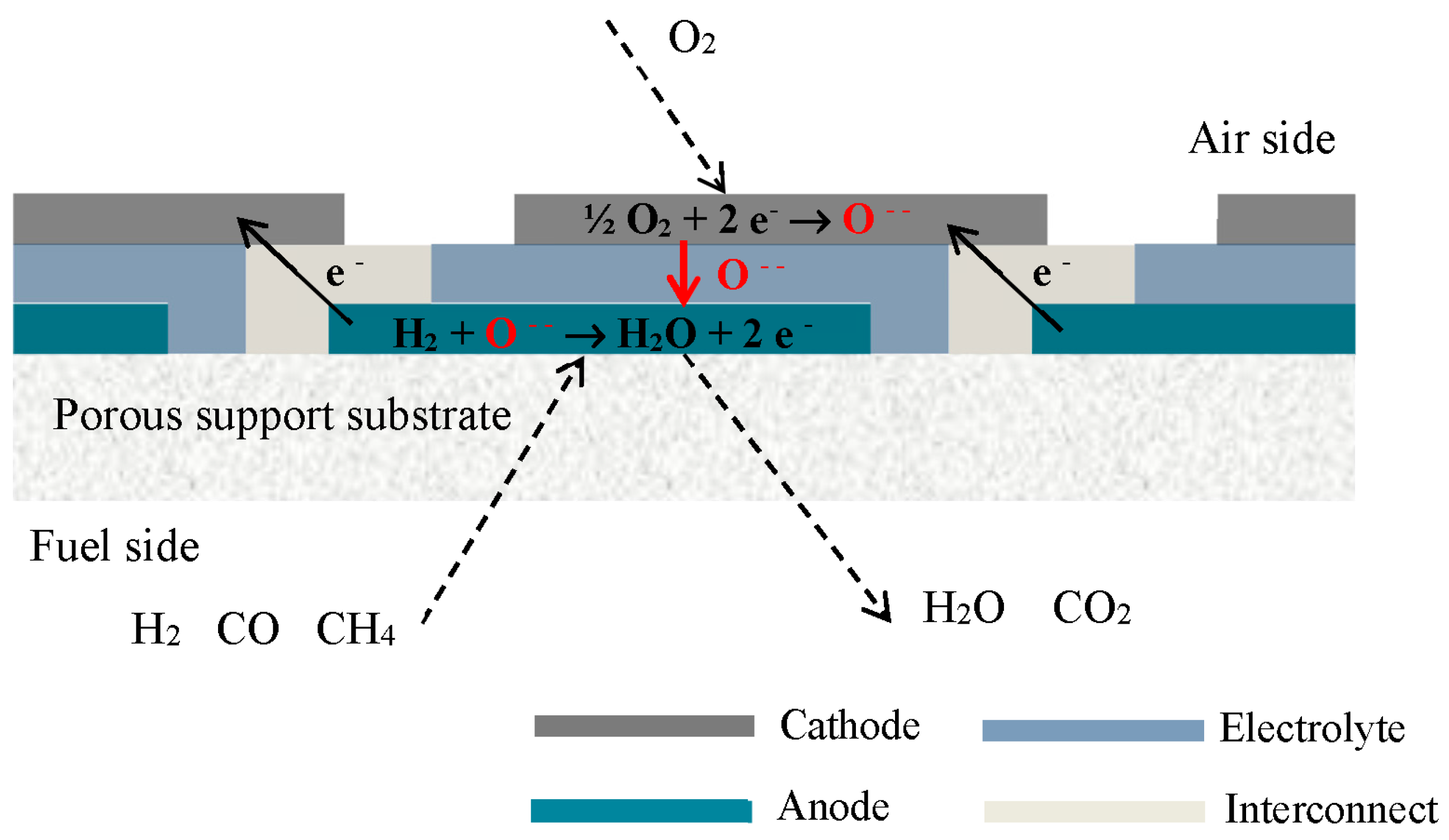
:1. Introduction


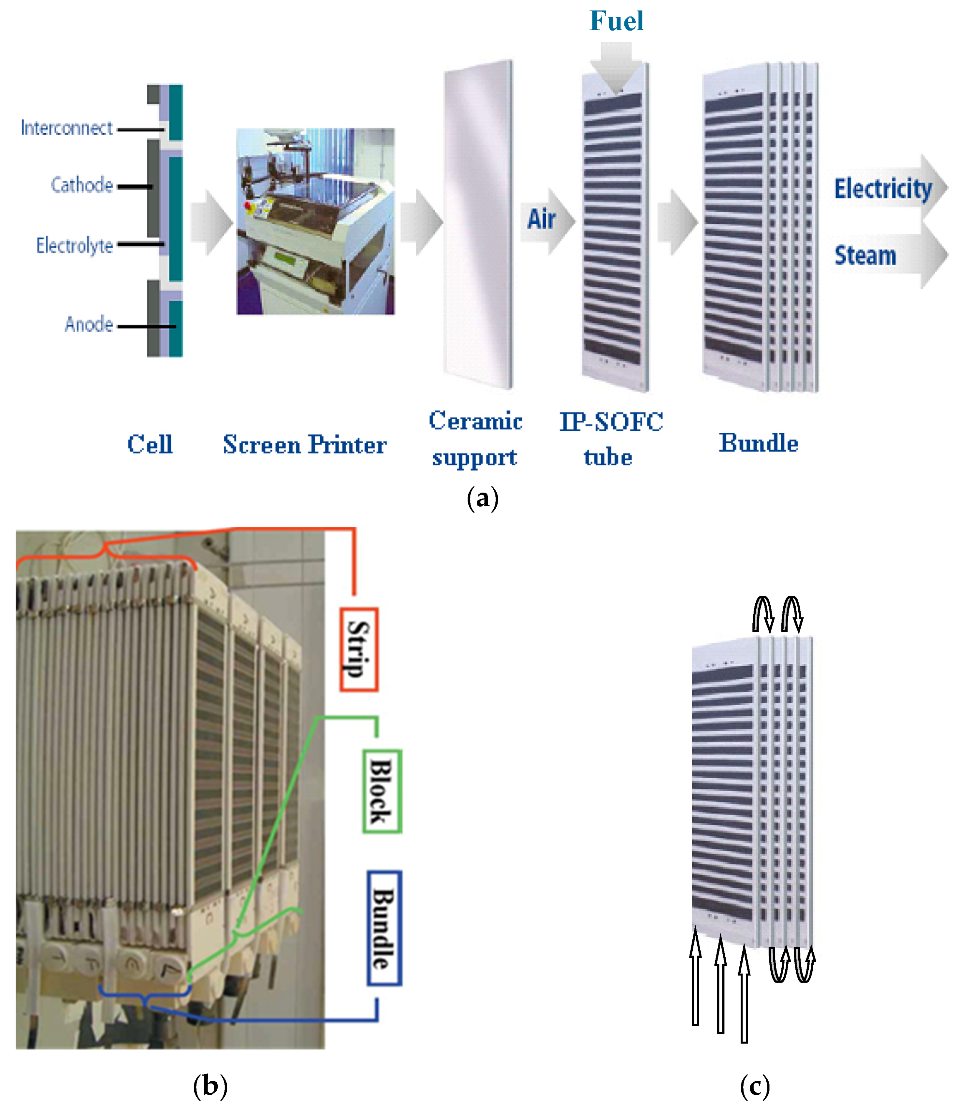
2. Experimental Setup

| Geometry | Datum |
|---|---|
| Number of tubes in the bundle (-) | 10 |
| Number of cells on each face of the tube (-) | 15 |
| Tube size (×10−3 m) | 280 × 68 |
| Tube thickness (×10−3 m) | 3.5 |
| Tube porosity (-) | 0.3 |
| Active cell size (×10−3 m) | 9 × 60 |
| Interconnection size (×10−3 m) | 6.25 × 60 |
| Number of anodic channels | 15 |
| Width of one anodic channel (×10−3 m) | 3.47 |
| Thickness of one anodic channel (×10−3 m) | 1.8 |
| Width of one cathodic channel (×10−3 m) | 280 |
| Thickness of one cathodic channel (×10−3 m) | 2 |
3. Mathematical Model
3.1. Model Development
- Heat exchange by radiation (i) between gases and solid in each single tube and (ii) between facing tubes inside the bundle has been neglected. Heat exchange of any type between tubes or bundles and the surrounding environment is neglected.
- Gravitational effects are not taken into account.
- A uniform distribution of the anodic flow rate among the inner channels of the tubes is assumed.
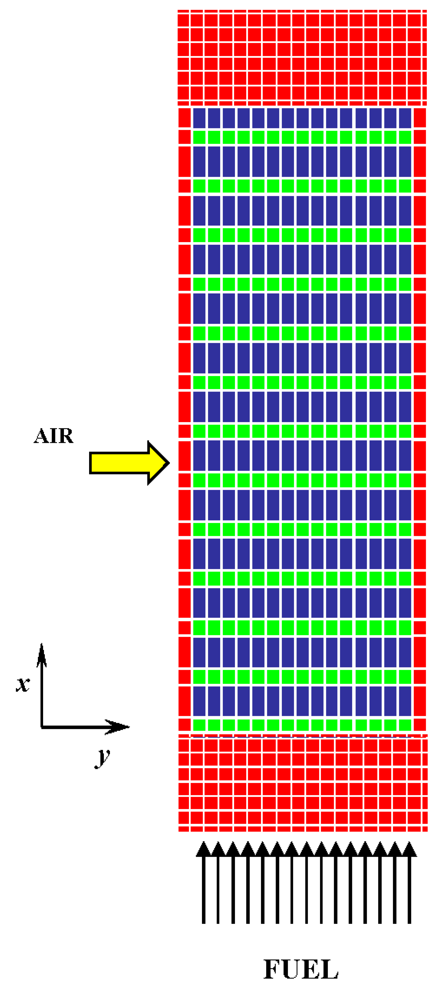
- The air flows only in the y direction with no transversal flows; moreover, the total inlet flow rate is equally subdivided among the bundle cathodic channels.
- All of the single cells supply the same electrical current. Both voltage and current are zero over the inactive edges of the tubes.
- Voltage can be considered uniform over each interconnection and active cell, due to the presence of elements with high electrical conductivity.
- Mass and energy balances of the gas streams are written in plug-flow form along their flow directions, because, even if the flow regime is laminar, the Péclet number is at least 20.
- MSR and WGS reactions are assumed at equilibrium in the anode channels.
- No carbon deposition is considered in the anode.
- The electrochemical oxidation of H2 is the only electrochemical reaction occurring at the anode.
- The bundle is simulated as a sequence of a number of tubes, placed one after the other.

3.1.1. Local Electrochemical Kinetics
3.1.2. Mass Balances
3.1.3. Energy Balances of the Gases
3.1.4. Energy Balance of the Solid
3.2. Geometry Discretization
3.3. Modelling Heat Conduction through the Solid Structure
3.4. Model Integration
3.5. Model Inputs and Outputs
| Operating parameter | Datum |
|---|---|
| Fuel flowrate (NL/min) | 6 |
| Oxidant (air) flowrate (NL/min) | 500 |
| Fuel inlet temperature (°C) | 930 |
| Air inlet temperature (°C) | 910 |
| Pressure (atm) | 1 |
4. Results and Discussion
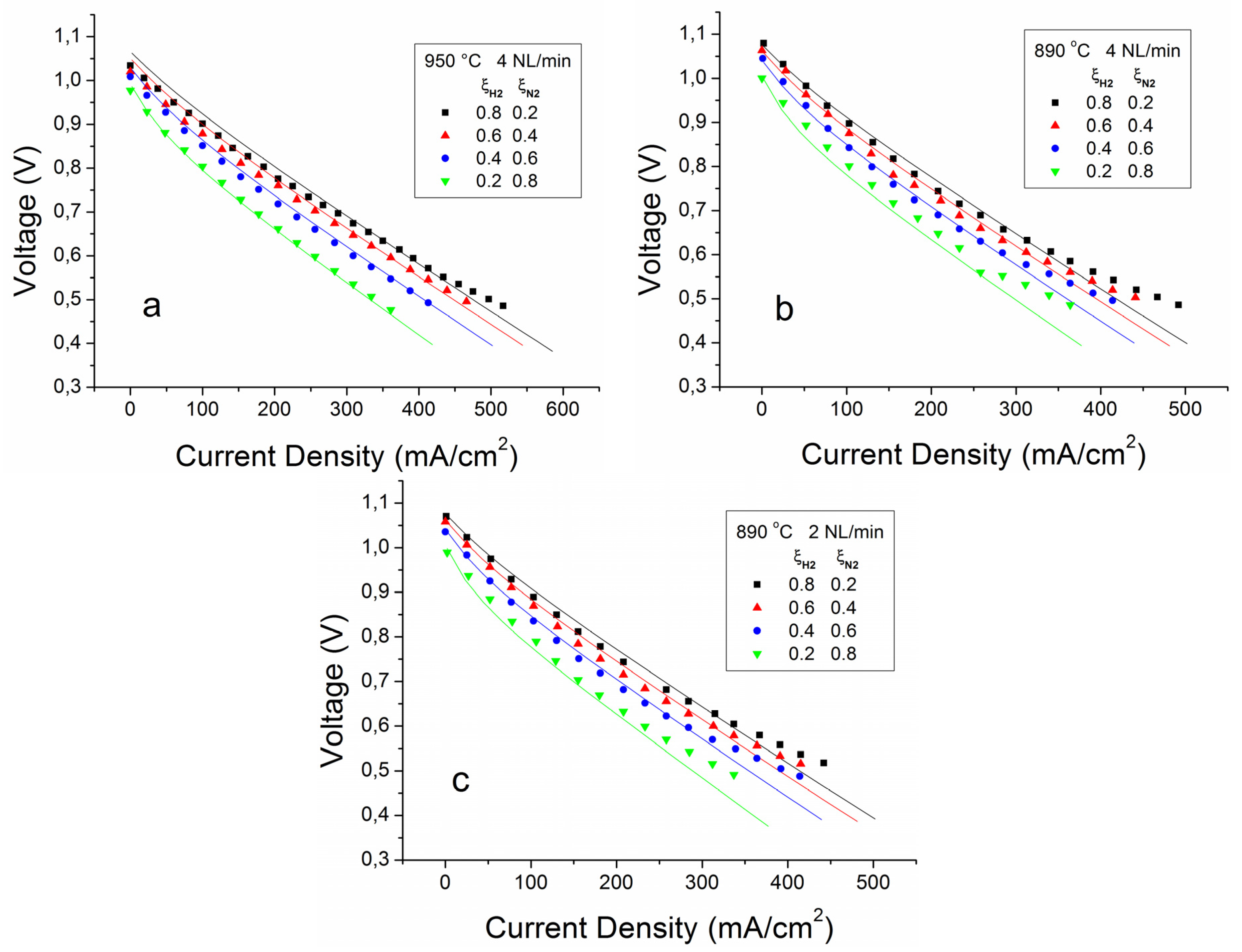
4.1. Model Validation
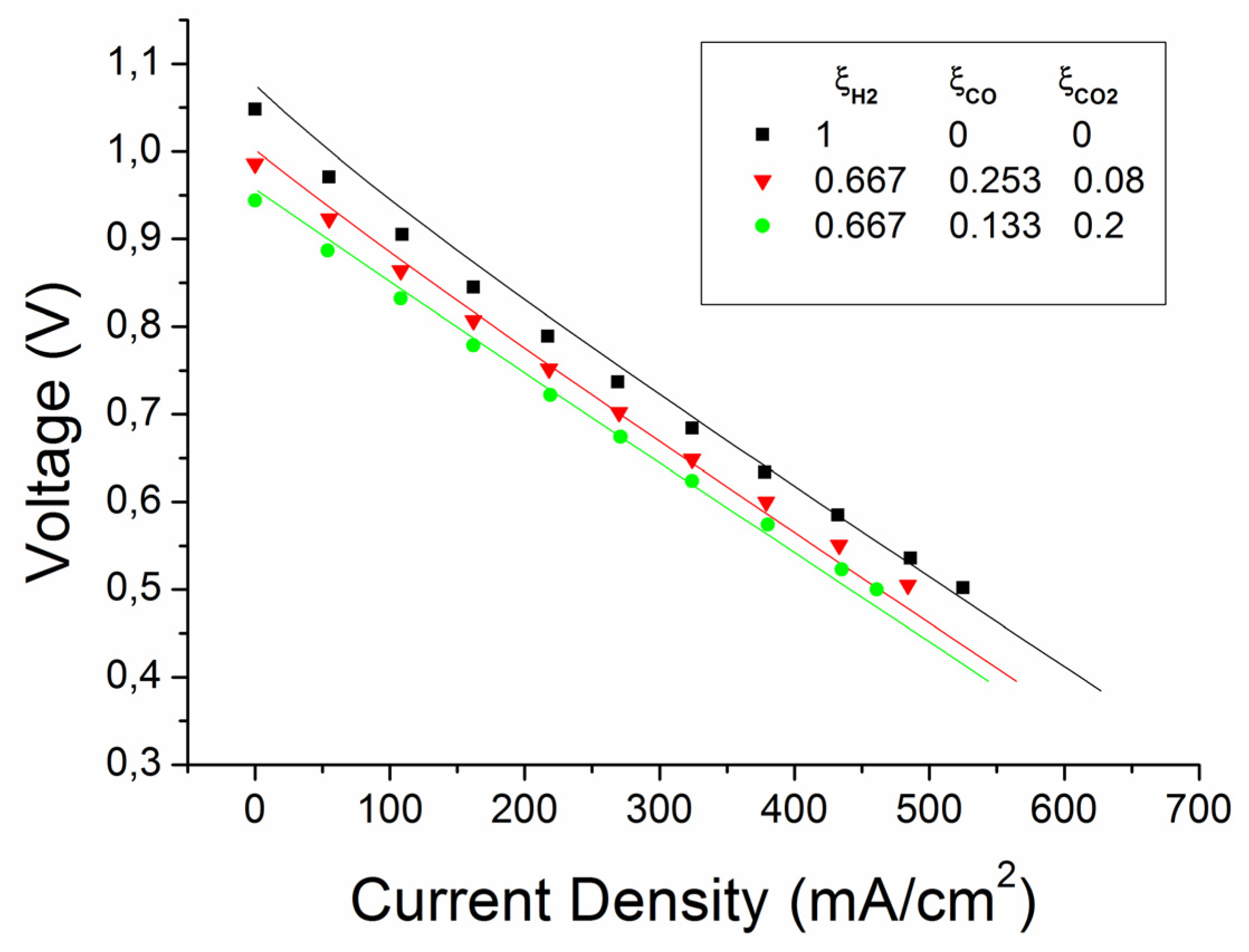
4.1.1. Validation with Binary Mixtures at the Anodic Side

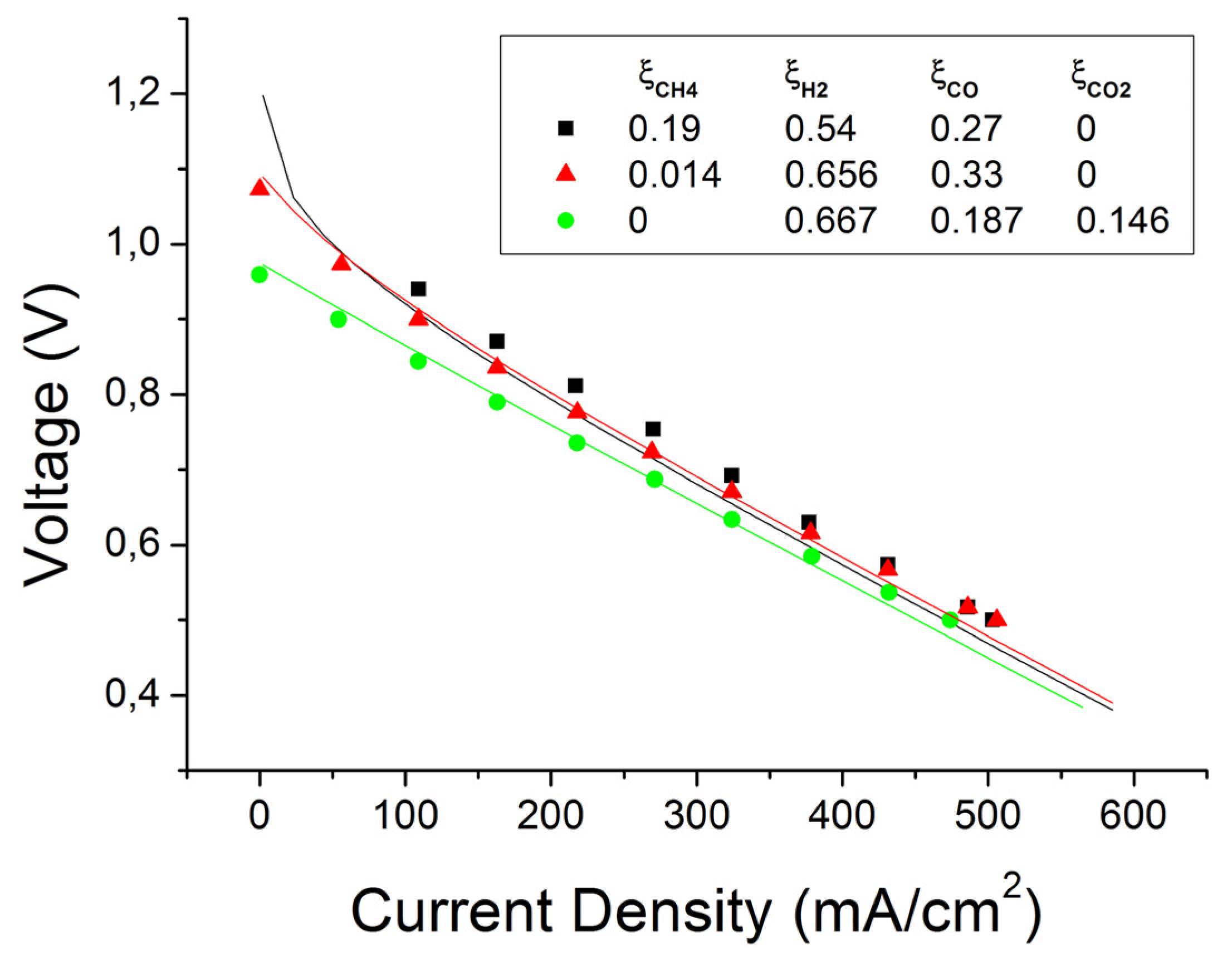
4.1.2. Further Validations
| Case | Feeding fuel composition (dry) | Feeding fuel composition (after humidification) | Fuel composition (after humidification and WGS reaction) | |||||||||
|---|---|---|---|---|---|---|---|---|---|---|---|---|
| ξH2 | ξH2O | ξCO | ξCO2 | ξH2 | ξH2O | ξCO | ξCO2 | ξH2 | ξH2O | ξCO | ξCO2 | |
| 1 | 1 | 0 | 0 | 0 | 0.97 | 0.03 | 0 | 0 | 0.97 | 0.03 | 0 | 0 |
| 2 | 0.667 | 0 | 0.253 | 0.08 | 0.647 | 0.03 | 0.245 | 0.078 | 0.599 | 0.078 | 0.292 | 0.031 |
| 3 | 0.667 | 0 | 0.133 | 0.2 | 0.647 | 0.03 | 0.129 | 0.194 | 0.517 | 0.16 | 0.258 | 0.065 |
| Case | Feeding fuel composition (dry) | Fuel composition (after humidification, WGS and MSR reactions) | ||||||||
|---|---|---|---|---|---|---|---|---|---|---|
| ξCH4 | ξH2 | ξH2O | ξCO | ξCO2 | ξCH4 | ξH2 | ξH2O | ξCO | ξCO2 | |
| 1 | 0.19 | 0.54 | 0 | 0.27 | 0 | 0.147 | 0.578 | 1.5 × 10⁻⁶ | 0.275 | 5.2 × 10⁻⁷ |
| 2 | 0.014 | 0.656 | 0 | 0.33 | 0 | 0.003 | 0.66 | 0.013 | 0.319 | 0.005 |
| 3 | 0 | 0.667 | 0 | 0.187 | 0.146 | 1.5 × 10⁻⁶ | 0.552 | 0.125 | 0.277 | 0.046 |
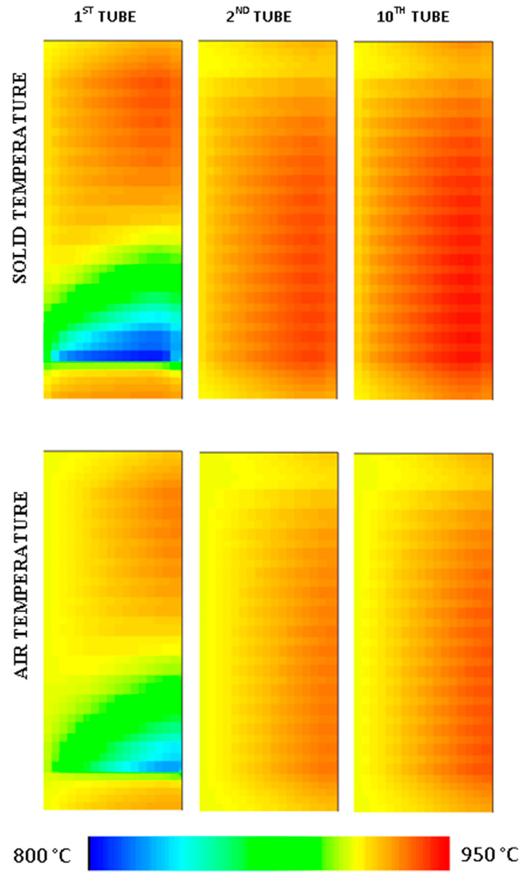
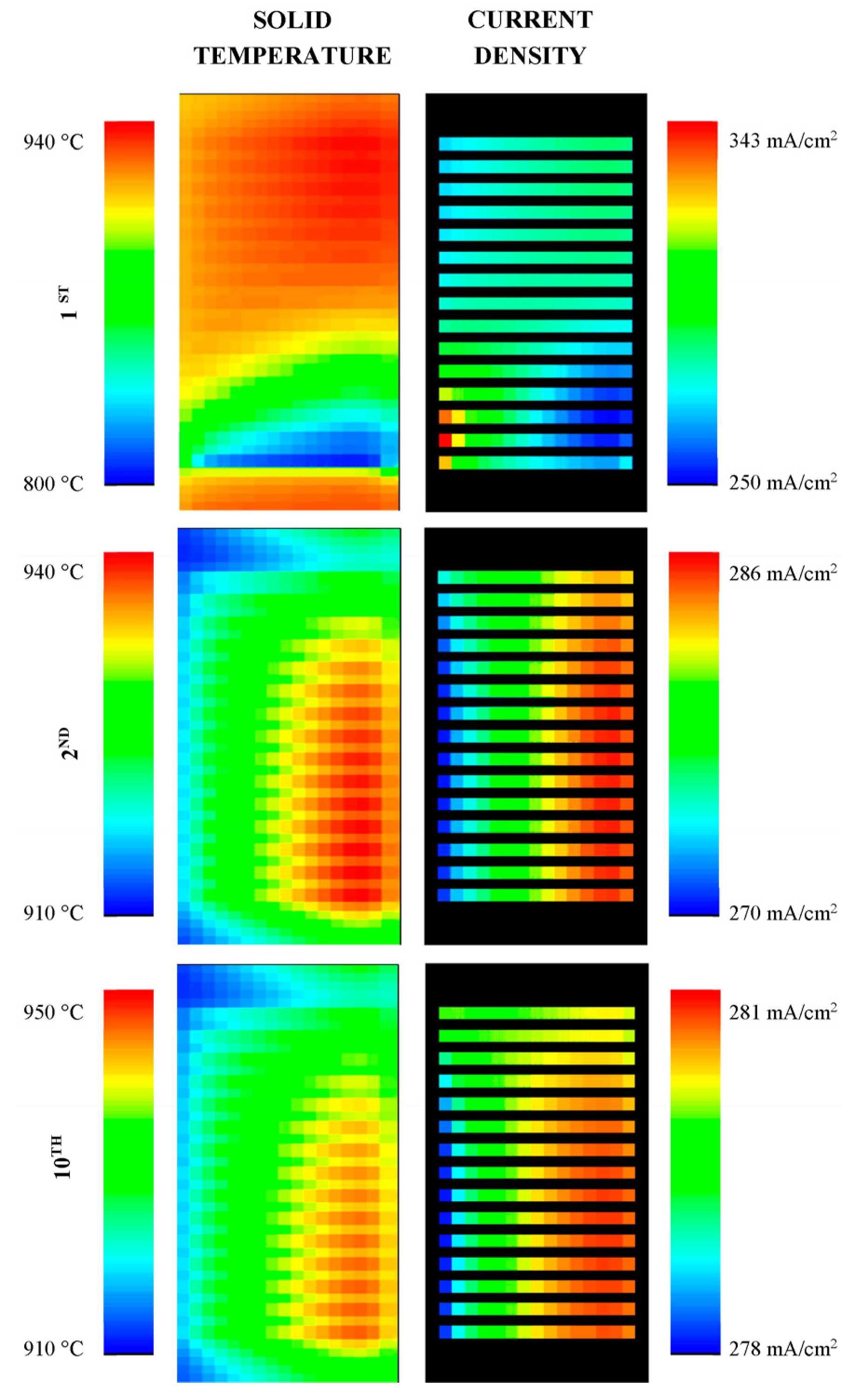
4.2. Model Predictions

5. Conclusions
Notation
| Symbols | |
| b | gas channel thickness (m) |
| B | ratio gas-solid heat exchange area/cell area (-) |
| cp | molar specific heat (J·mol−1·K−1) |
| d1, d2 | distances between centres of adjacent mesh elements (m) |
| dh | hydraulic diameter (m) |
| dt | time step (s) |
| Eact | activation energy (J·mol−1) |
| F | Faraday constant (A·s·mol−1) |
| ΔG | Gibbs free energy change of the overall reaction (J·mol−1) |
| ΔG° | standard Gibbs free energy change of the overall reaction (J·mol−1) |
| h | heat transfer coefficient (W·m−2·K−1) |
| ΔH | enthalpy change of the overall reaction (J·mol−1) |
| i0 | exchange current density (A·m−2) |
| k | electrical current density (A·m−2) |
| k | thermal conductivity (W·m−1·K−1) |
| K | thermal conductivity of layered solid (W·m−1·K−1) |
| L | width of stripe of tube fed by one anodic gas channel (m) |
| nch | number of channels (-) |
| ne | number of electrons transferred in the electrochemical reaction |
| Nu | Nusselt number (-) |
| p | partial pressure (Pa) |
| Rg | gas constant (J·mol−1·K) |
| Rth | thermal resistivity of layered solid (W−1·m·K) |
| r | reaction rate (mol·m−3·s−1) |
| s | overall solid thickness (m) |
| t | layer thickness (m) |
| T | temperature (K) |
| V | electrical potential (V) |
| W | molar flow rate (mol·m−2·s−1) |
| x, y | coordinates (m) |
| Greek letters | |
| ε | porosity (-) |
| γ | pre-exponential factor (A·m−2) |
| η | potential loss (V) |
| λ | gas heat conductivity (W·m−1·K−1) |
| ν | stoichiometric coefficient (-) |
| ξ | mole fraction (-) |
| Subscript | |
| a | anode |
| act | activation |
| c | cathode |
| conc | concentration |
| eff | effective |
| i | i-th component |
| j | j-th reaction |
| Nernst | Nernst |
| ohm | ohmic |
| s | solid |
| st | supporting tube |
| Superscript | |
| ° | bulk flow of gases |
| MSR | methane steam reforming reaction |
| WGS | water gas shifting reaction |
Acknowledgments
Author Contributions
Conflicts of Interest
References
- Singhal, S.C.; Kendall, K. High Temperature Solid Oxide Fuel Cells: Fundamentals, Design and Applications; Elsevier: Philadelphia, PA, USA, 2003. [Google Scholar]
- Srinivasan, S. Fuel Cells: From Fundamentals to Applications; Springer: Berlin, Germany, 2006. [Google Scholar]
- Brett, D.J.L.; Atkinson, A.; Brandon, N.P.; Skinner, S.J. Intermediate temperature solid oxide fuel cells. Chem. Soc. Rev. 2008, 37, 1568–1578. [Google Scholar] [CrossRef] [PubMed]
- Tietz, F. Solid Oxide Fuel Cells, Encyclopedia of Materials: Science and Technology; Elsevier: Philadelphia, PA, USA, 2008; pp. 1–8. [Google Scholar]
- Appleby, A.J. Fuel Cells—Overview, in Encyclopedia of Electrochemical Power Sources; Elsevier: Philadelphia, PA, USA, 2009; pp. 277–296. [Google Scholar]
- Wu, J.; Liu, X. Recent Development of SOFC metallic interconnect. J. Mater. Sci. Technol. 2010, 26, 293–305. [Google Scholar] [CrossRef]
- Behling, N. Fuel Cells: Current Technology Challenges and Future Research Need; Elsevier: Philadelphia, PA, USA, 2012. [Google Scholar]
- Huang, K.; Singhal, S.C. Cathode-supported tubular solid oxide fuel cell technology: A critical review. J. Power Sources 2013, 237, 84–97. [Google Scholar] [CrossRef]
- Gardner, F.J.; Day, M.J.; Brandon, N.P.; Pashley, M.N.; Cassidy, M. SOFC technology development at Rolls-Royce. J. Power Sources 2000, 86, 122–129. [Google Scholar] [CrossRef]
- Debenedetti, P.G.; Vayenas, C.G. Steady state analysis of high temperature fuel cells. Chem. Eng. Sci. 1983, 38, 1817–1829. [Google Scholar] [CrossRef]
- Vayenas, C.G.; Debenedetti, P.G.; Yentekakis, Y.; Hegedus, L.L. Cross-flow solid-state electrochemical reactors: A steady-state analysis. Ind. Eng. Chem. Fundam. 1985, 24, 316–324. [Google Scholar] [CrossRef]
- Bove, R.; Ubertini, S. (Eds.) Modeling Solid Oxide Fuel Cells: Methods, Procedures and Techniques; Springer: Berlin, Germany, 2008.
- Yuan, M.A.J.; Sudén, B. Review on modeling development for multiscale chemical reactions coupled transport phenomena in solid oxide fuel cells. Appl. Energy 2010, 87, 1461–1476. [Google Scholar] [CrossRef]
- Hajimolana, S.A.; Hussain, M.A.; Daud, W.M.A.W.; Soroush, M.; Shamiri, A. Mathematical modeling of solid oxide fuel cells: A review. Renew. Sustain Energy Rev. 2011, 15, 1893–1917. [Google Scholar] [CrossRef]
- Wang, K.; Hissel, D.; Péra, M.C.; Steiner, N.; Marra, D.; Sorrentino, M.; Pianese, C.; Monteverde, M.; Cardone, P.; Saarinen, J. A Review on solid oxide fuel cell models. Int. J. Hydrogen Energy 2011, 36, 7212–7228. [Google Scholar] [CrossRef]
- Grew, K.N.; Chiu, W.K.S. A review on modeling and simulation techniques across the length scales for the solid oxide fuel cell. J. Power Sources 2012, 199, 1–13. [Google Scholar] [CrossRef]
- Bhattacharyya, D.; Rengaswamy, R. A Review of Solid Oxide Fuel Cell (SOFC) Dynamic Models. Ind. Eng. Chem. Res. 2009, 48, 6068–6086. [Google Scholar] [CrossRef]
- Costamagna, P.; Selimovic, A.; del Borghi, M.; Agnew, G. Electrochemical Model of the Integrated Planar Solid Oxide Fuel Cell (IP-SOFC). Chem. Eng. J. 2004, 102, 61–69. [Google Scholar] [CrossRef]
- Cui, D.; Cheng, M. Design for segmented-in-series solid oxide fuel cell through mathematical modelling. J. Power Sources 2010, 195, 1435–1440. [Google Scholar] [CrossRef]
- Haberman, B.A.; Young, J.B. A detailed three-dimensional simulation of an IP-SOFC stack. J. Fuel Cell Sci. Tech. 2008, 5. [Google Scholar] [CrossRef]
- Mounir, H.; El Gharad, A.; Belaiche, M.; Boukalouch, M. Thermo-fluid and electrochemical modeling of a multi-bundle IP-SOFC—Technology for second generation hybrid application. Energy Convers. Manag. 2009, 50, 2685–2692. [Google Scholar] [CrossRef]
- Magistri, L.; Costamagna, P.; Massardo, A.F. A hybrid system based on a personal turbine (5 kW) and a solid oxide fuel cell stack: A flexible and high efficiency energy concept for the distributed power market. J. Eng. Gas Turbine Power 2002, 124, 850–857. [Google Scholar] [CrossRef]
- Magistri, L.; Traverso, A.; Cerutti, F.; Bozzolo, M.; Costamagna, P.; Massardo, A.F. Modelling of pressurised hybrid systems based on integrated planar solid oxide fuel cell (IP-SOFC) technology. Fuel Cells 2005, 5, 80–96. [Google Scholar] [CrossRef]
- Trasino, F.; Bozzolo, M.; Magistri, L.; Massardo, A.F. Modeling and performance analysis of the Rolls-Royce fuel cell systems limited: 1 MW plant. J. Eng. Gas Turbine Power 2011, 133. [Google Scholar] [CrossRef]
- Costamagna, P.; Arato, E.; Antonucci, P.L.; Antonucci, V. Partial oxidation of CH4 in solid oxide fuel cells: Simulation model of the electrochemical reactor and experimental validation. Chem. Eng. Sci. 1996, 51, 3013–3018. [Google Scholar] [CrossRef]
- Yurkiv, V. Reformate-operated SOFC anode performance and degradation considering solid carbon formation: A modeling and simulation study. Electrochim. Acta 2014, 143, 114–128. [Google Scholar] [CrossRef]
- Day, T.; Singdeo, D.; Bose, M.; Basu, R.N.; Ghosh, P.C. Study of contact resistance at the electrode-interconnect interfaces in planar type solid oxide fuel cells. J. Power Sources 2013, 233, 290–298. [Google Scholar] [CrossRef]
- Costamagna, P.; Honegger, K. Modeling of solid oxide heat exchanger integrated stacks and simulation at high fuel utilization. J. Electrochem. Soc. 1998, 145, 3995–4007. [Google Scholar] [CrossRef]
- Noren, D.A.; Hoffman, M.A. Clarifying the butler-volmer equation and related approximations for calculating activation losses in solid oxide fuel cell models. J. Power Sources 2005, 152, 175–181. [Google Scholar] [CrossRef]
- Wang, Z.; Wang, Z.; Yang, W.; Peng, R.; Lu, Y. Carbon-tolerant solid oxide fuel cells using NiTiO3 as an anode internal reformer. J. Power Sources 2014, 255, 404–409. [Google Scholar] [CrossRef]
- Bossel, U.G. Facts and Figures: IEA Task Report; Swiss Federal Office of Energy: Berne, Switzerland, 1992.
- Perry, R.H.; Green, D.W. Perry’s Chemical Engineers’ Handbook, 8th ed.; McGraw-Hill: New York, NY, USA, 2007. [Google Scholar]
- Mogensen, D.; Grunwaldt, J.-D.; Hendriksen, P.V.; Dam-Johansen, K.; Nielsen, J.U. Internal steam reforming in solid oxide fuel cells: Status and opportunities of kinetic studies and their impact on modelling. J. Power Sources 2011, 196, 25–38. [Google Scholar] [CrossRef]
- Tseronis, K.; Kookos, I.K.; Theodoropoulos, C. Modelling mass transport in solid oxide fuel cell anodes: A case for a multidimensional dusty gas-based model. Chem. Eng. Sci. 2008, 63, 5626–5638. [Google Scholar] [CrossRef]
- Paradis, H.; Andersson, M.; Yuan, J.; Sundén, B. CFD modeling: Different kinetic approaches for internal reforming reactions in an anode-sopported SOFC. J. Fuel Cell Sci. Technol. 2011, 8. [Google Scholar] [CrossRef]
- Achenbach, E.; Riensche, E. Methane/steam redorming kinetics for solid oxide fuel cells. J. Power Sources 1994, 52, 283–288. [Google Scholar] [CrossRef]
- Janardhanan, V.M.; Heuveline, V.; Deutschmann, O. Performance analysis of a SOFC under direct internal reforming conditions. J. Power Sources 2007, 172, 296–307. [Google Scholar] [CrossRef]
- Aguiar, P.; Adjiman, C.S.; Brandon, N.P. Anode-supported intermediate temperature direct internal reforming solid oxide fuel cell. I: Model-based steady-state performance. J. Power Sources 2004, 138, 120–136. [Google Scholar] [CrossRef]
- Clague, R.; Marquis, A.J.; Brandon, N.P. Finite element and analytical stress analysis of a solid oxide fuel cell. J. Power Sources 2012, 210, 224–232. [Google Scholar] [CrossRef]
- Clague, R.; Marquis, A.J.; Brandon, N.P. Time independent and time dependent probability of failure of solid oxide fuel cells by stress analysis and the Weibull method. J. Power Sources 2013, 221, 290–299. [Google Scholar] [CrossRef]
© 2015 by the authors; licensee MDPI, Basel, Switzerland. This article is an open access article distributed under the terms and conditions of the Creative Commons by Attribution (CC-BY) license (http://creativecommons.org/licenses/by/4.0/).
Share and Cite
Costamagna, P.; Grosso, S.; Travis, R.; Magistri, L. Integrated Planar Solid Oxide Fuel Cell: Steady-State Model of a Bundle and Validation through Single Tube Experimental Data. Energies 2015, 8, 13231-13254. https://doi.org/10.3390/en81112364
Costamagna P, Grosso S, Travis R, Magistri L. Integrated Planar Solid Oxide Fuel Cell: Steady-State Model of a Bundle and Validation through Single Tube Experimental Data. Energies. 2015; 8(11):13231-13254. https://doi.org/10.3390/en81112364
Chicago/Turabian StyleCostamagna, Paola, Simone Grosso, Rowland Travis, and Loredana Magistri. 2015. "Integrated Planar Solid Oxide Fuel Cell: Steady-State Model of a Bundle and Validation through Single Tube Experimental Data" Energies 8, no. 11: 13231-13254. https://doi.org/10.3390/en81112364