
Comparing World Economic and Net Energy Metrics, Part 2: Total Economy Expenditure Perspective

Abstract
:1. Introduction
1.1. Background
1.2. Part 2 Goal and Content
1.3. Input-Output (I-O) Frameworks: Economic and Energy Analysis
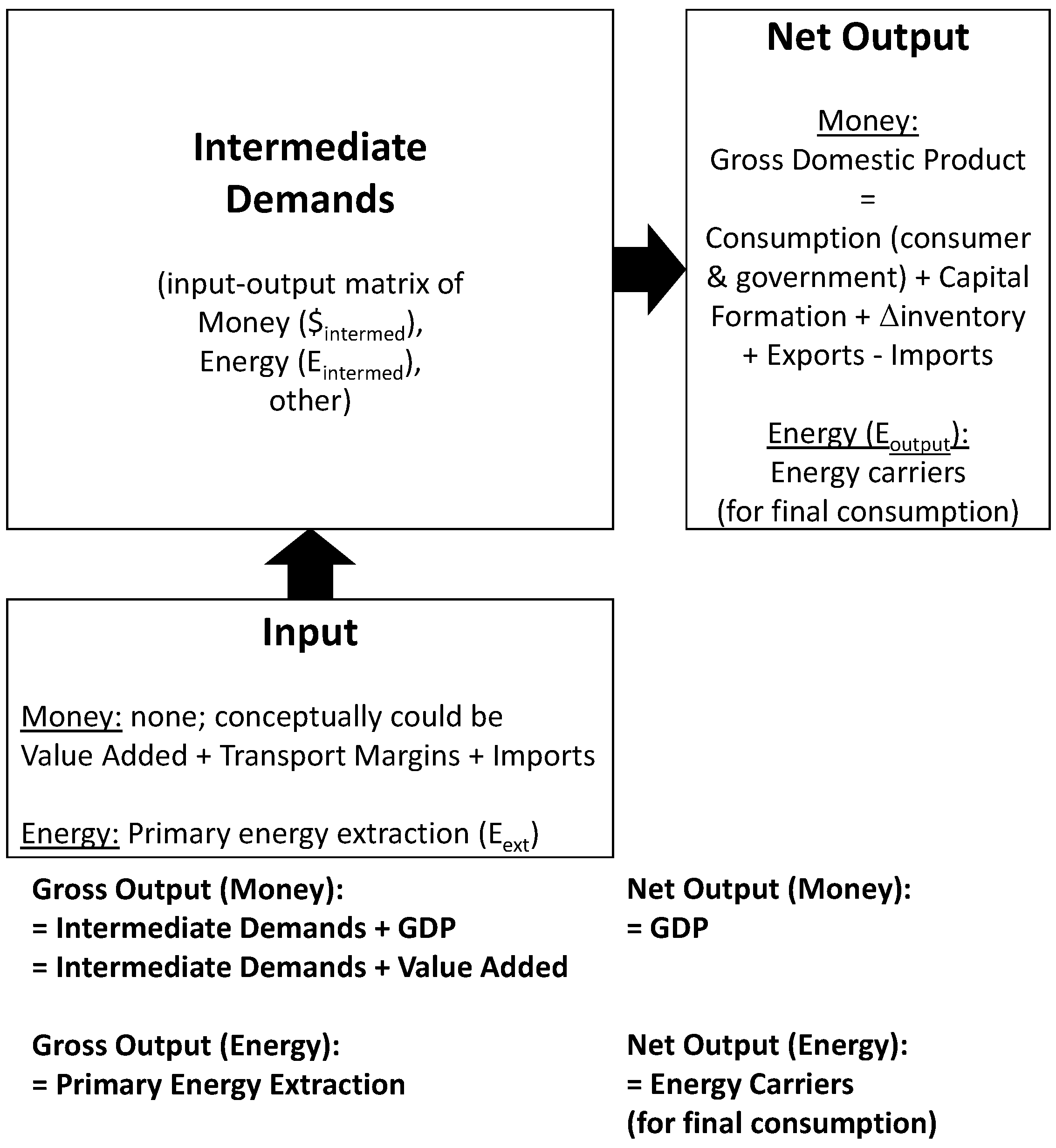
1.3.1. Economic Analysis Framework
1.3.2. Energy Analysis Framework
1.3.3. I-O Frameworks Compared: Money Ratios Compared to Energy and Power Return Ratios

| Process | Final | Total | |
|---|---|---|---|
| Sector | Demand | Output | |
| Process Sector | |||
| Payments Sector | |||
| Total Outlays | = |
2. Methods
2.1. Definitions of Energy and Power Return Ratios
2.2. Monetary Expenditures on Energy
2.2.1. IEA Data

2.2.2. Estimating Intermediate Expenditures on Energy from I-O Tables (World Input-Output Database)
2.3. Direct Energy Input PRRs
3. Results
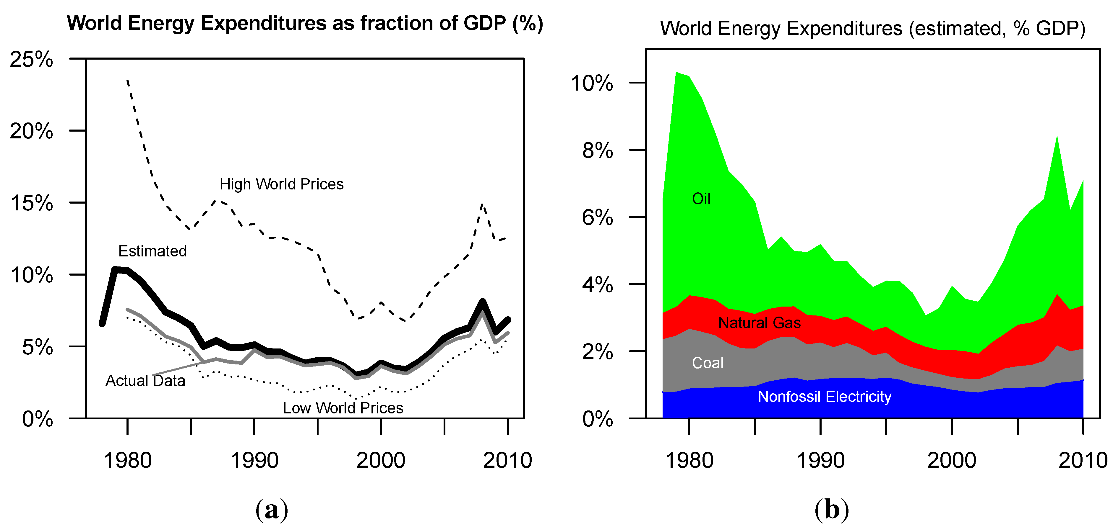
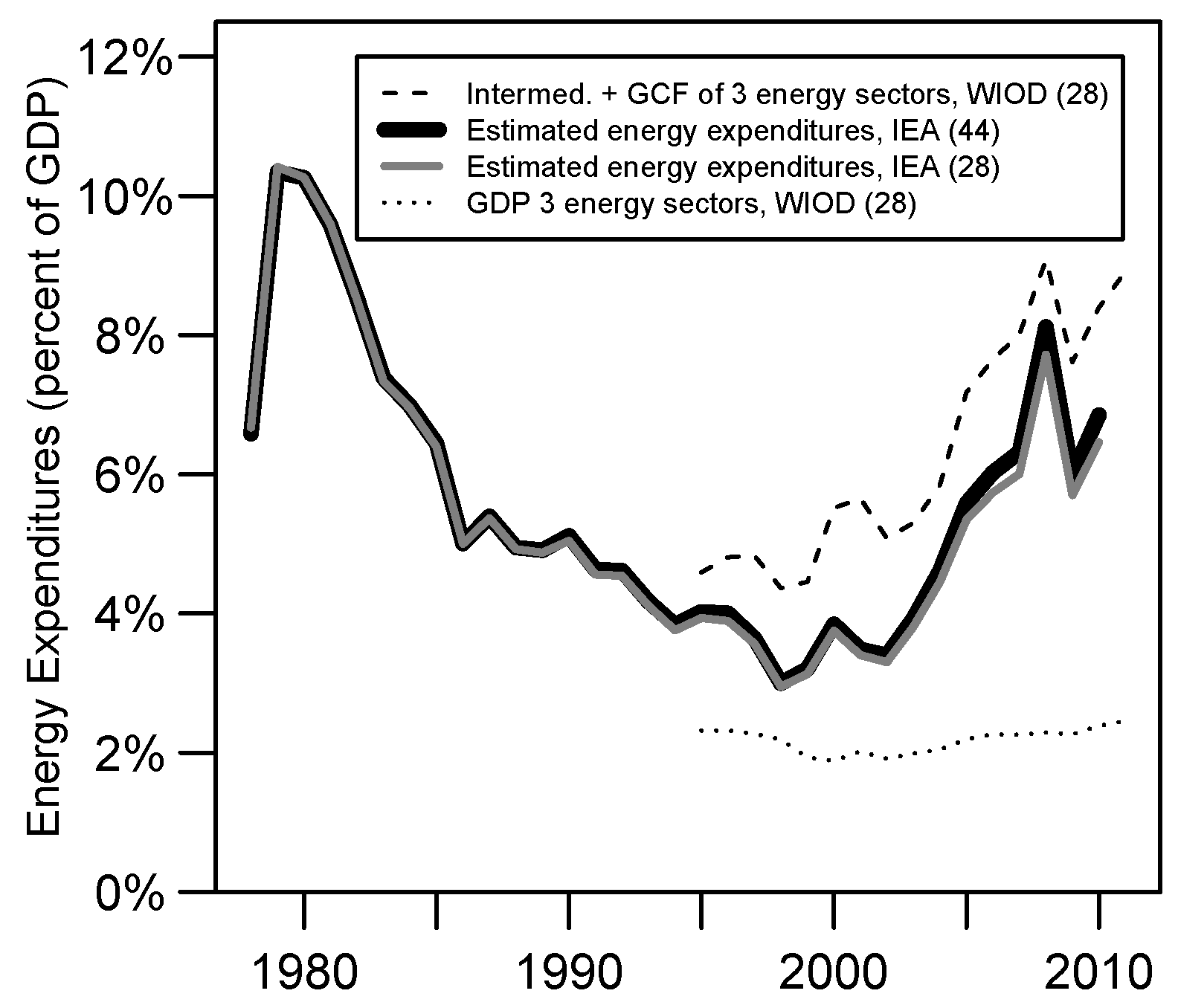
- The estimated , using IEA data, decreased from a maximum of 10.3% in 1979 to 3.0% in 1998 before increasing to 8.1% in 2008.
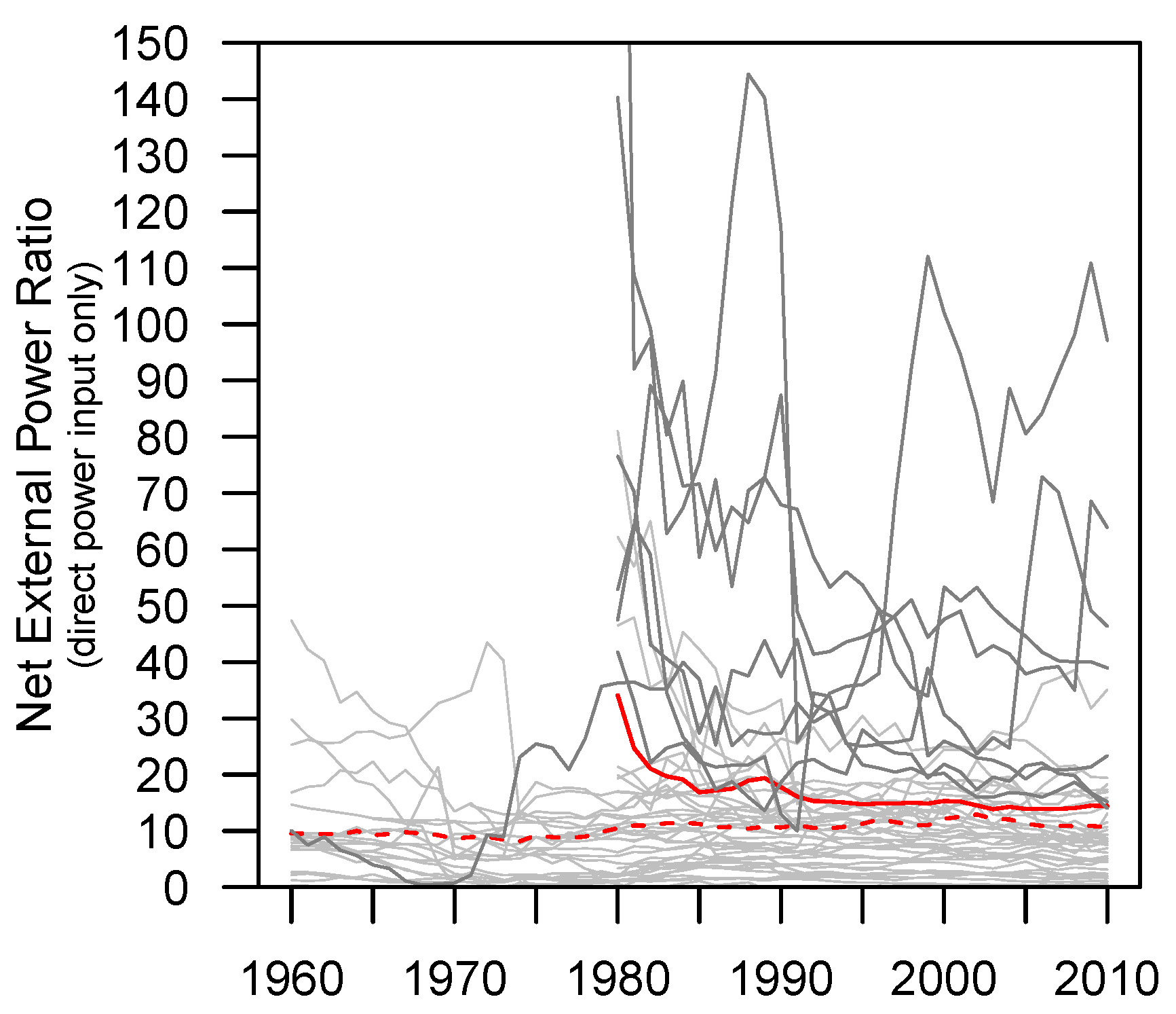
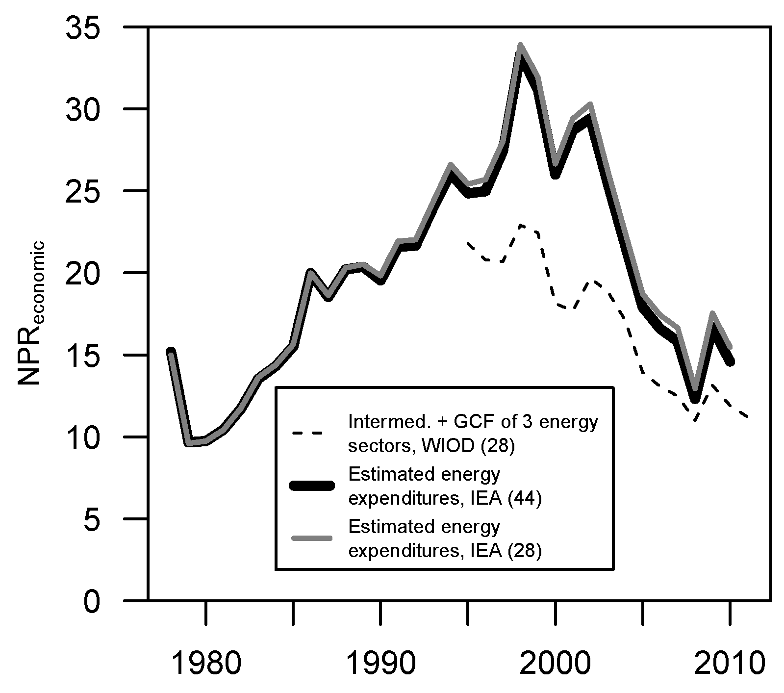
- NEPR declined from a value of 34 in 1980 to 17 in 1986 before staying in a range between 14 and 16 from 1991–2010.
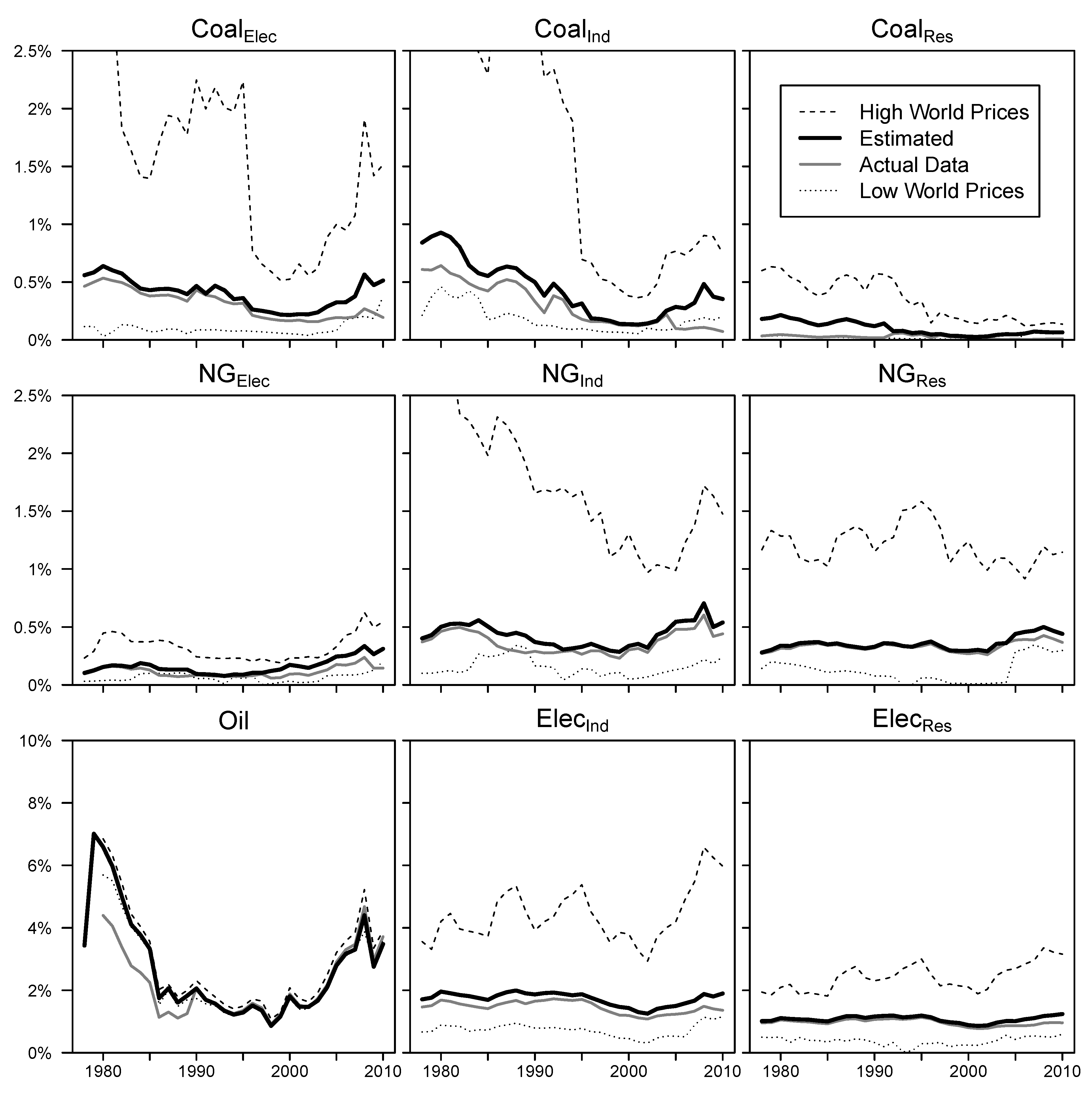
3.1. Expenditures on Energy/GDP =

3.2. NEPR

4. Discussion
4.1. Context of as Economy-Wide Power Return Ratio, NPR


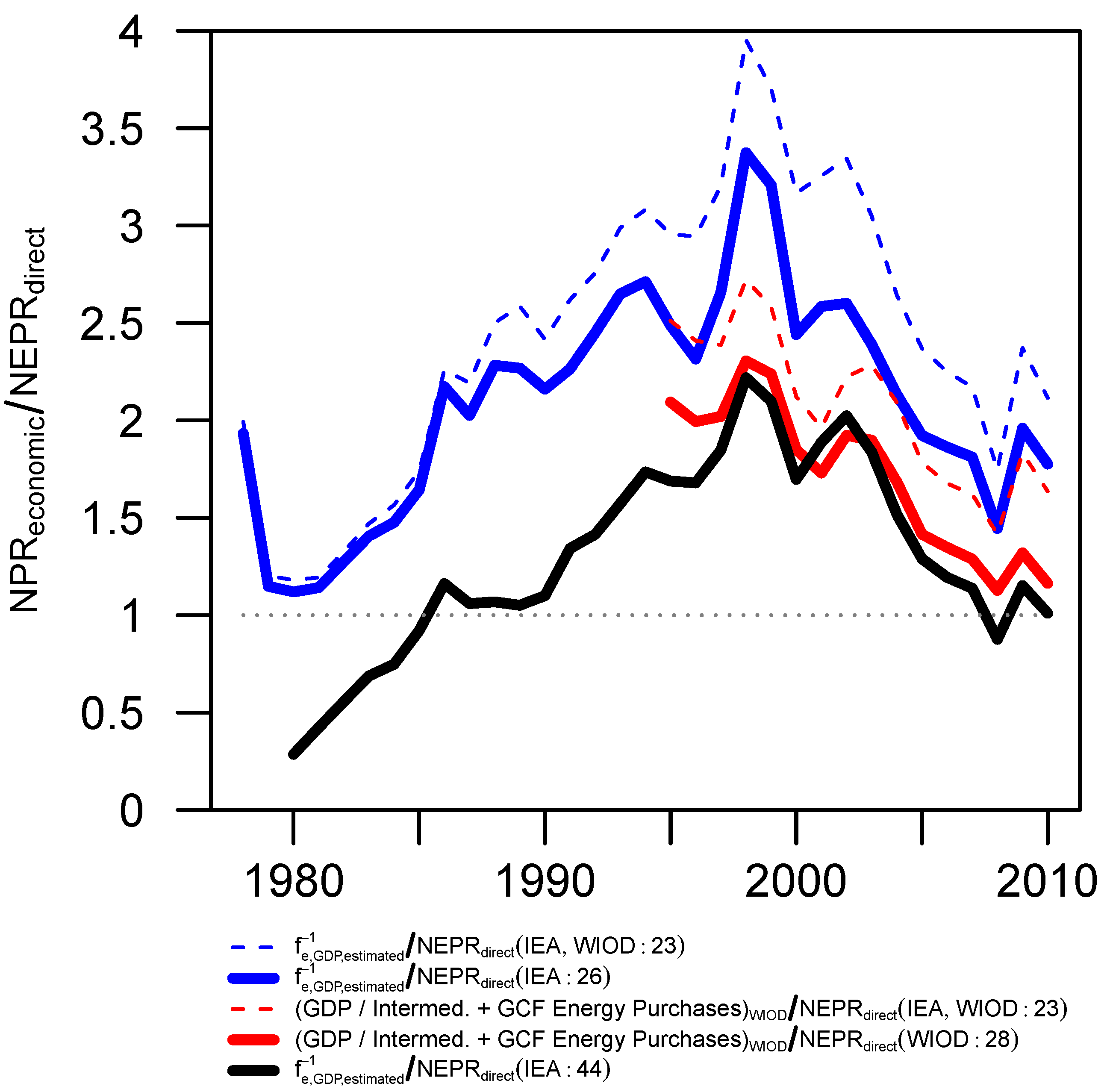
4.2. NEPR Relative to
- for our data, Inequality (7) is not generally true over the studied time period,
- including more countries, particularly net energy exporters, in the analysis decreases the NPRNEPR ratio moving it closer to affirming our hypothesis in Inequality (7),
- using the data from the World Input-Output Database (three-sector energy-related intermediate expenditures plus capital expenditures as gross capital formation) decreases the NPRNEPR ratio, moving it closer to affirming our hypothesis in Inequality (7) and,
- the temporal pattern is driven primarily by variation in monetary expenditures for energy and not the calculation of NEPR.

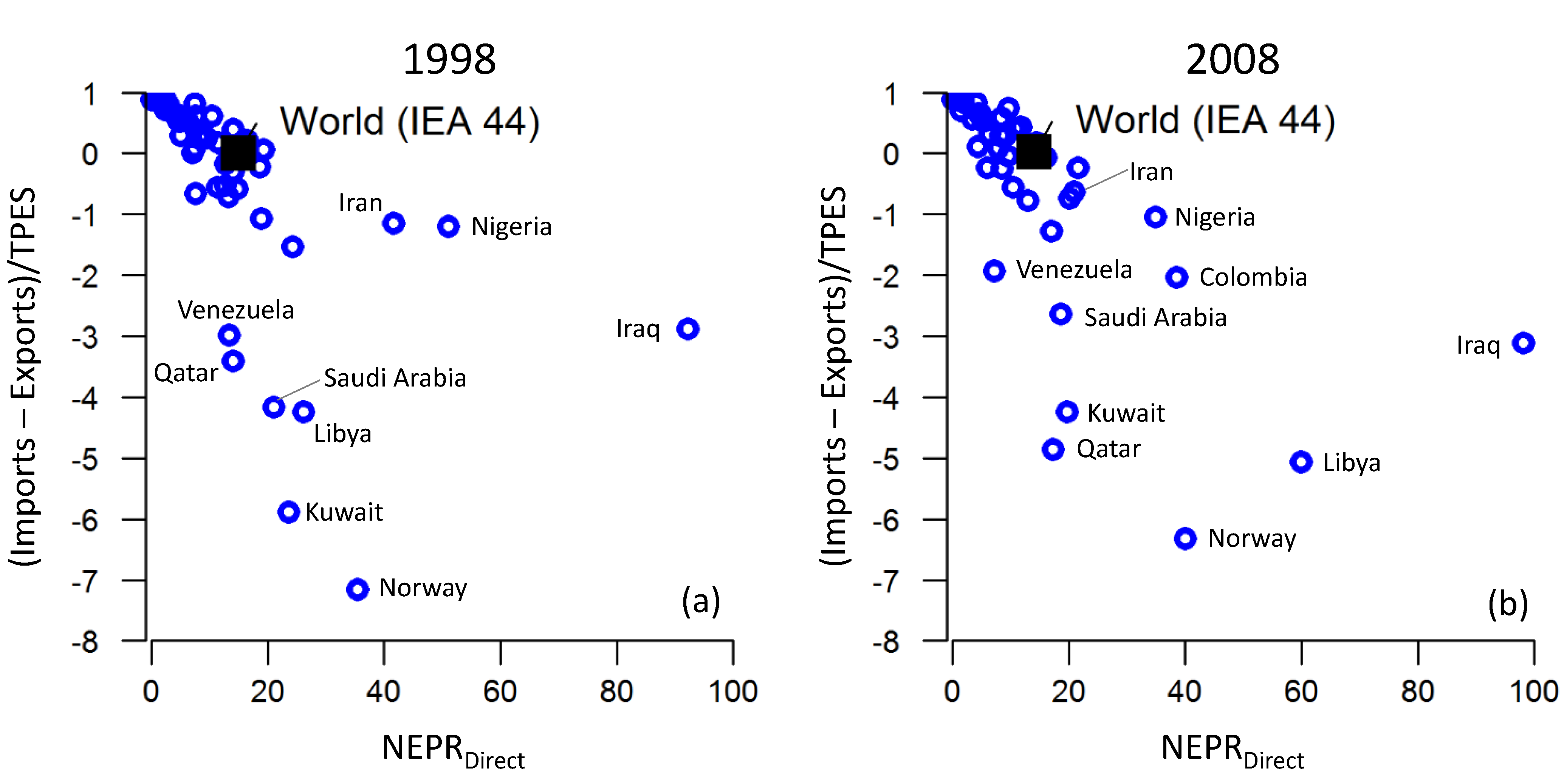
4.3. Relation between Net Energy Imports and NEPR
5. Conclusions
Supplementary Files
Supplementary File 1Supplementary File 2Acknowledgments
Author Contributions
Conflicts of Interest
References
- King, C.W.; Maxwell, J.P.; Donovan, A. Comparing world economic and net energy metrics, Part 1: Price Perspective. Energies 2015, 8, 12949–12974. [Google Scholar] [CrossRef]
- King, C.W. Comparing world economic and net energy metrics, Part 3: Macroeconomic Historical and Future Perspectives. Energies 2015, 8, 12997–13020. [Google Scholar] [CrossRef]
- Solow, R. A Contribution to the Theory of Economic-Growth. Q. J. Econ. 1956, 70, 65–94. [Google Scholar] [CrossRef]
- Hamilton, J. Historical Oil Shocks. In Routledge Handbook of Major Events in Economic History; Parker, R.E., Whaples, R.M., Eds.; Routledge: New York, NY, USA, 2013; p. 239265. [Google Scholar]
- Ayres, R.; Voudouris, V. The economic growth enigma: Capital, labour and useful energy? Energy Policy 2014, 64, 16–28. [Google Scholar] [CrossRef]
- Voudouris, V.; Ayres, R.; Serrenho, A.C.; Kiose, D. The economic growth enigma revisited: The EU-15 since the 1970s. Energy Policy 2015, 86, 812–832. [Google Scholar] [CrossRef]
- Kander, A.; Stern, D.I. Economic growth and the transition from traditional to modern energy in Sweden. Energy Econ. 2014, 46, 56–65. [Google Scholar] [CrossRef]
- Kümmel, R. The Second Law of Economics: Energy, Entropy, and the Origins of Wealth; Springer: Berlin, Germnay, 2011. [Google Scholar]
- Hall, C.A.S.; Klitgaard, K.A. Energy and the Wealth of Nations: Understanding the Biophysical Economy, 1st ed.; Springer: Berlin, Germnay, 2012. [Google Scholar]
- Ayres, R.U. Sustainability economics: Where do we stand? Ecol. Econ. 2008, 67, 281–310. [Google Scholar] [CrossRef]
- Brown, J.H.; Burnside, W.R.; Davidson, A.D.; Delong, J.R.; Dunn, W.C.; Hamilton, M.J.; Mercado-Silva, N.; Nekola, J.C.; Okie, J.G.; Woodruff, W.H.; et al. Energetic Limits to Economic Growth. BioScience 2011, 61, 19–26. [Google Scholar] [CrossRef]
- Peters, G.P.; Hertwich, E.G. CO2 embodied in international trade with implications for global climate policy. Environ. Sci. Technol. 2008, 42, 1401–1407. [Google Scholar] [CrossRef] [PubMed]
- Acemoglu, D.; Robinson, J.A. Why Nations Fail: The Origins of Power, Prosperity, and Poverty; Crown Business: New York, NY, USA, 2012. [Google Scholar]
- Tainter, J. The Collapse of Complex Societies; Cambridge University Press: Cambridge, UK, 1988. [Google Scholar]
- Tainter, J.A. Energy, complexity, and sustainability: A historical perspective. Environ. Innov. Soc. Transit. 2011, 1, 89–95. [Google Scholar] [CrossRef]
- Tainter, J.A. Energy and Existential Sustainability: The Role of Reserve Capacity. J. Environ. Account. Manag. 2013, 1, 213–228. [Google Scholar] [CrossRef]
- Turchin, P.; Nefedov, S.A. Secular Cycles; Princeston University Press: Princeton, NJ, USA, 2009. [Google Scholar]
- Ayres, R.U.; Warr, B. Accounting for growth: The role of physical work. Struct. Chang. Econ. Dyn. 2005, 16, 181–209. [Google Scholar] [CrossRef]
- Stern, D.; Kander, A. The Role of Energy in the Industrial Revolution and Modern Economic Growth; Technical Report; The Australian National University: Canberra, Australia, 2011. [Google Scholar]
- Stern, D.I.; Kander, A. The Role of Energy in the Industrial Revolution and Modern Economic Growth. Energy J. 2012, 33, 125–152. [Google Scholar] [CrossRef]
- Hamilton, J. Causes and Consequences of the Oil Shock of 2007-08. In Brookings Papers on Economic Activity; Romer, D., Wolfers, J., Eds.; Brookings Institution Press: Washington, DC, USA, 2009; p. 69. [Google Scholar]
- Hall, C.A.S.; Cleveland, C.J.; Kaufmann, R.K. Energy and Resource Quality: The Ecology of the Economic Process; Wiley: New York, NY, USA, 1986. [Google Scholar]
- Hall, C.A.S.; Balogh, S.; Murphy, D.J.R. What is the Minimum EROI that a Sustainable Society Must Have? Energies 2009, 2, 25–47. [Google Scholar] [CrossRef]
- King, C.W. Energy intensity ratios as net energy measures of United States energy production and expenditures. Environ. Res. Lett. 2010, 5, 044006. [Google Scholar] [CrossRef]
- Brandt, A.R. Converting oil shale to liquid fuels: Energy inputs and greenhouse gas emissions of the Shell in situ conversion process. Environ. Sci. Technol. 2008, 42, 7489–7495. [Google Scholar] [CrossRef] [PubMed]
- Brandt, A.R. Converting Oil Shale to Liquid Fuels with the Alberta Taciuk Processor: Energy Inputs and Greenhouse Gas Emissions. Energy Fuels 2009, 23, 6253–6258. [Google Scholar] [CrossRef]
- Brandt, A.R.; Englander, J.; Bharadwaj, S. The energy efficiency of oil sands extraction: Energy return ratios from 1970 to 2010. Energy 2013, 55, 693–702. [Google Scholar] [CrossRef]
- Guilford, M.C.; Hall, C.A.S.; O’Connor, P.; Cleveland, C.J. A New Long Term Assessment of Energy Return on Investment (EROI) for U.S. Oil and Gas Discovery and Production. Sustainability 2011, 3, 1866–1887. [Google Scholar] [CrossRef]
- Farrell, A.E.; Plevin, R.J.; Turner, B.T.; Jones, A.D.; O’Hare, M.; Kammen, D.M. Ethanol can contribute to energy and environmental goals. Science 2006, 311, 506–508. [Google Scholar] [CrossRef] [PubMed]
- Raugei, M.; Fullana-i-Palmer, P.; Fthenakis, V. The energy return on energy investment (EROI) of photovoltaics: Methodology and comparisons with fossil fuel life cycles. Energy Policy 2012, 45, 576–582. [Google Scholar] [CrossRef]
- Dale, M.; Benson, S.M. Energy Balance of the Global Photovoltaic (PV) Industry—Is the PV Industry a Net Electricity Producer? Environ. Sci. Technol. 2013, 47, pp. 3482–3489. Available online: http://pubs.acs.org/doi/pdf/10.1021/es3038824 (accessed on 3 March 2015). [CrossRef] [PubMed]
- Fthenakis, V.M.; Kim, H.C. Photovoltaics: Life-cycle analyses. Sol. Energy 2011, 85, 1609–1628. [Google Scholar] [CrossRef]
- Zhang, Y.; Colosi, L.M. Practical ambiguities during calculation of energy ratios and their impacts on life cycle assessment calculations. Energy Policy 2013, 57, 630–633. [Google Scholar] [CrossRef]
- Bullard, C.W., III; Herendeen, R.A. The energy cost of goods and services. Energy Policy 1975, 3, 268–278. [Google Scholar] [CrossRef]
- Costanza, R. Embodied Energy and Economic Valuation. Science 1980, 210, 1219–1224. [Google Scholar] [CrossRef] [PubMed]
- King, C.W.; Hall, C.A.S. Relating Financial and Energy Return on Investment. Sustainability 2011, 3, 1810–1832. [Google Scholar] [CrossRef]
- Henshaw, P.F.; King, C.; Zarnikau, J. System Energy Assessment (SEA), Defining a Standard Measure of EROI for Energy Businesses as Whole Systems. Sustainability 2011, 3, 1908–1943. [Google Scholar] [CrossRef]
- Miller, R.E.; Blair, P.D. Input-Output Analysis: Foundations and Extensions; Cambridge University Press: Cambridge, UK, 2009. [Google Scholar]
- Casler, S.; Wilbur, S. Energy Input-Output Analysis: A Simple Guide. Resour. Energy 1984, 6, 187–201. [Google Scholar] [CrossRef]
- Bullard, C.W.; Penner, P.S.; Pilati, D.A. Net energy analysis: Handbook for combining process and input-output analysis. Resour. Energy 1978, 1, 267–313. [Google Scholar] [CrossRef]
- King, C.W. Matrix method for comparing system and individual energy return ratios when considering an energy transition. Energy 2014, 72, 254–265. [Google Scholar] [CrossRef]
- Brandt, A.R.; Dale, M.; Barnhart, C.J. Calculating systems-scale energy efficiency and net energy returns: A bottom-up matrix-based approach. Energy 2013, 62, 235–247. [Google Scholar] [CrossRef]
- Brandt, A.R.; Dale, M. A General Mathematical Framework for Calculating Systems-Scale Efficiency of Energy Extraction and Conversion: Energy Return on Investment (EROI) and Other Energy Return Ratios. Energies 2011, 4, 1211–1245. [Google Scholar] [CrossRef]
- Murphy, D.J.R.; Hall, C.A.S.; Dale, M.; Cleveland, C.J. Order from Chaos: A Preliminary Protocol for Determining EROI for fuels. Sustainability 2011, 3, 1888–1907. [Google Scholar] [CrossRef]
- Modahl, I.S.; Raadal, H.L.; Gagnon, L.; Bakken, T.H. How methodological issues affect the energy indicator results for different electricity generation technologies. Energy Policy 2013, 63, 283–299. [Google Scholar] [CrossRef]
- Herendeen, R.A. Connecting net energy with the price of energy and other goods and services. Ecol. Econ. 2015, 109, 142–149. [Google Scholar] [CrossRef]
- Timmer, M.P.; Dietzenbacher, E.; Los, B.; Stehrer, R.; de Vries, G.J. An Illustrated User Guide to the World Input–Output Database: The Case of Global Automotive Production. Rev. Int. Econ. 2015, 23, 575–605. [Google Scholar] [CrossRef]
- O’Mahony, M.; Timmer, M.P. Output, Input and Productivity Measures at the Industry Level: The EU KLEMS Database. Econ. J. 2009, 119, F374–F403. [Google Scholar] [CrossRef]
- Dietzenbacher, E.; Los, B.; Stehrer, R.; Timmer, M.; de Vries, G. The Construction of World Input-Output Tables in the WIOD project. Econ. Syst. Res. 2013, 25, 71–98. [Google Scholar] [CrossRef]
- Sorrell, S.; Speirs, J. Using growth curves to forecast regional resource recovery: Approaches, analytics and consistency tests. Philos. Trans. R. Soc. A Math. Phys. Eng. Sci. 2014, 372. Available online: http://rsta.royalsocietypublishing.org/ content/372/2006/20120317.full.pdf+html (accessed on 3 March 2015). [CrossRef] [PubMed]
© 2015 by the authors; licensee MDPI, Basel, Switzerland. This article is an open access article distributed under the terms and conditions of the Creative Commons by Attribution (CC-BY) license (http://creativecommons.org/licenses/by/4.0/).
Share and Cite
King, C.W.; Maxwell, J.P.; Donovan, A. Comparing World Economic and Net Energy Metrics, Part 2: Total Economy Expenditure Perspective. Energies 2015, 8, 12975-12996. https://doi.org/10.3390/en81112347
King CW, Maxwell JP, Donovan A. Comparing World Economic and Net Energy Metrics, Part 2: Total Economy Expenditure Perspective. Energies. 2015; 8(11):12975-12996. https://doi.org/10.3390/en81112347
Chicago/Turabian StyleKing, Carey W., John P. Maxwell, and Alyssa Donovan. 2015. "Comparing World Economic and Net Energy Metrics, Part 2: Total Economy Expenditure Perspective" Energies 8, no. 11: 12975-12996. https://doi.org/10.3390/en81112347
APA StyleKing, C. W., Maxwell, J. P., & Donovan, A. (2015). Comparing World Economic and Net Energy Metrics, Part 2: Total Economy Expenditure Perspective. Energies, 8(11), 12975-12996. https://doi.org/10.3390/en81112347