
Comparing World Economic and Net Energy Metrics, Part 1: Single Technology and Commodity Perspective

Abstract
:1. Introduction
1.1. Background
1.2. Missing Perspective
1.3. Part 1 Goal and Content
1.4. Summary of Multidisciplinary Perspectives and Motivation
2. Methods
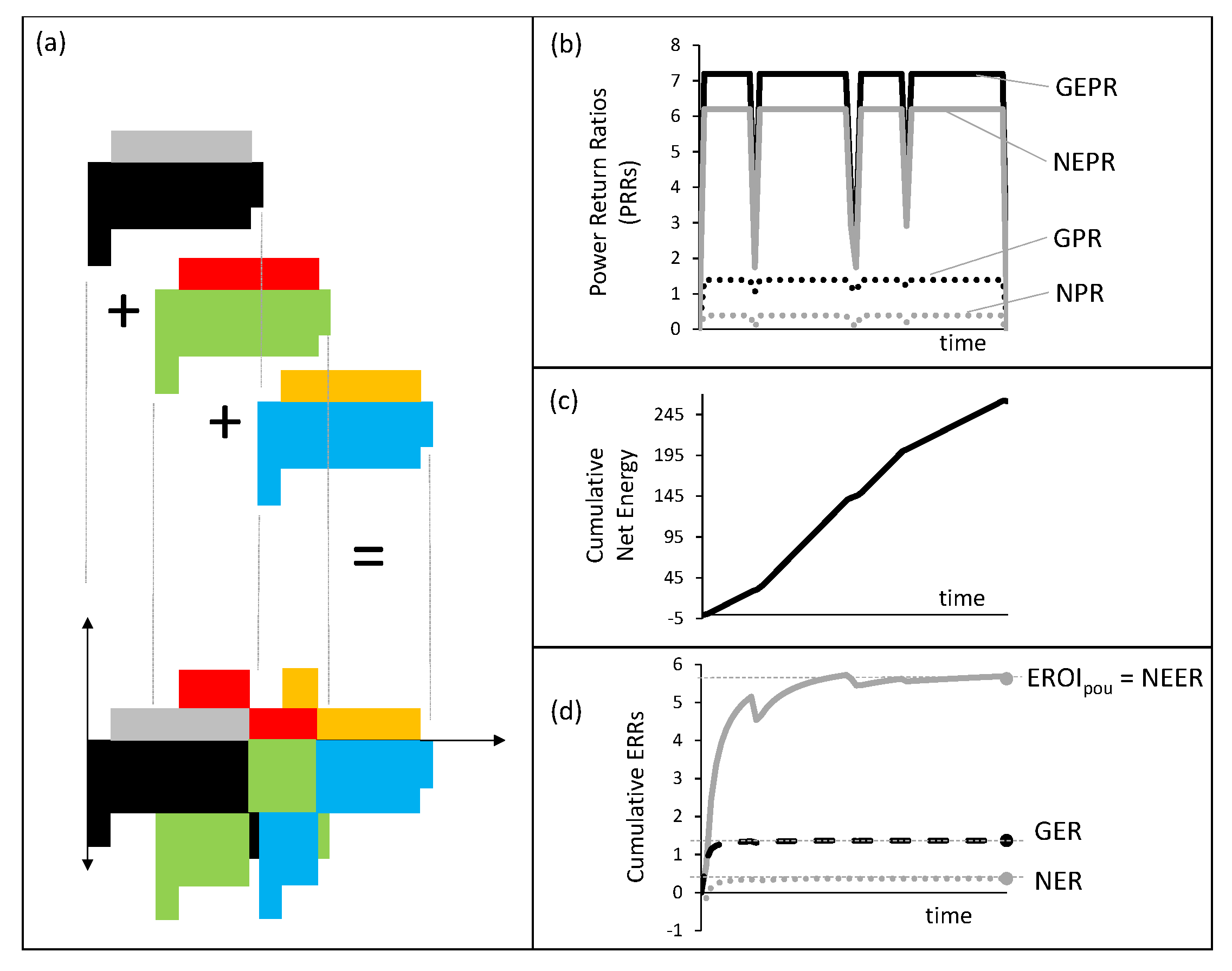
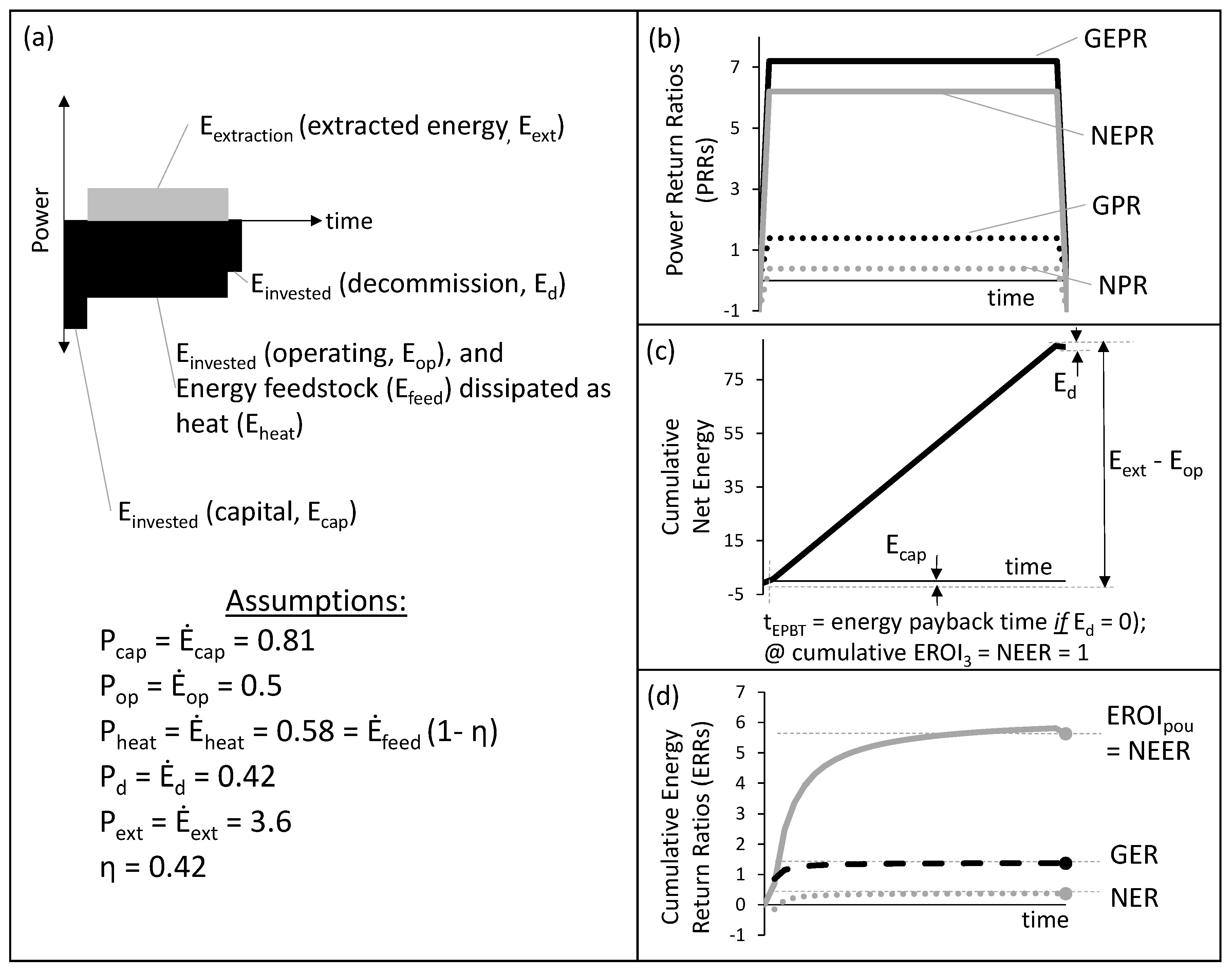
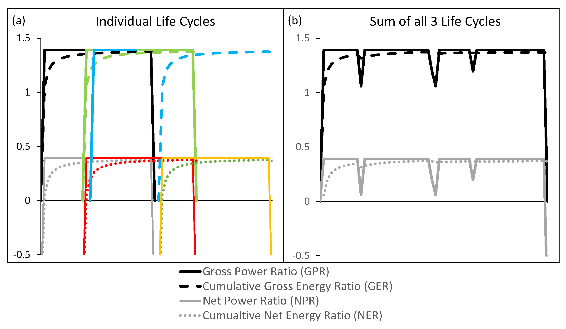
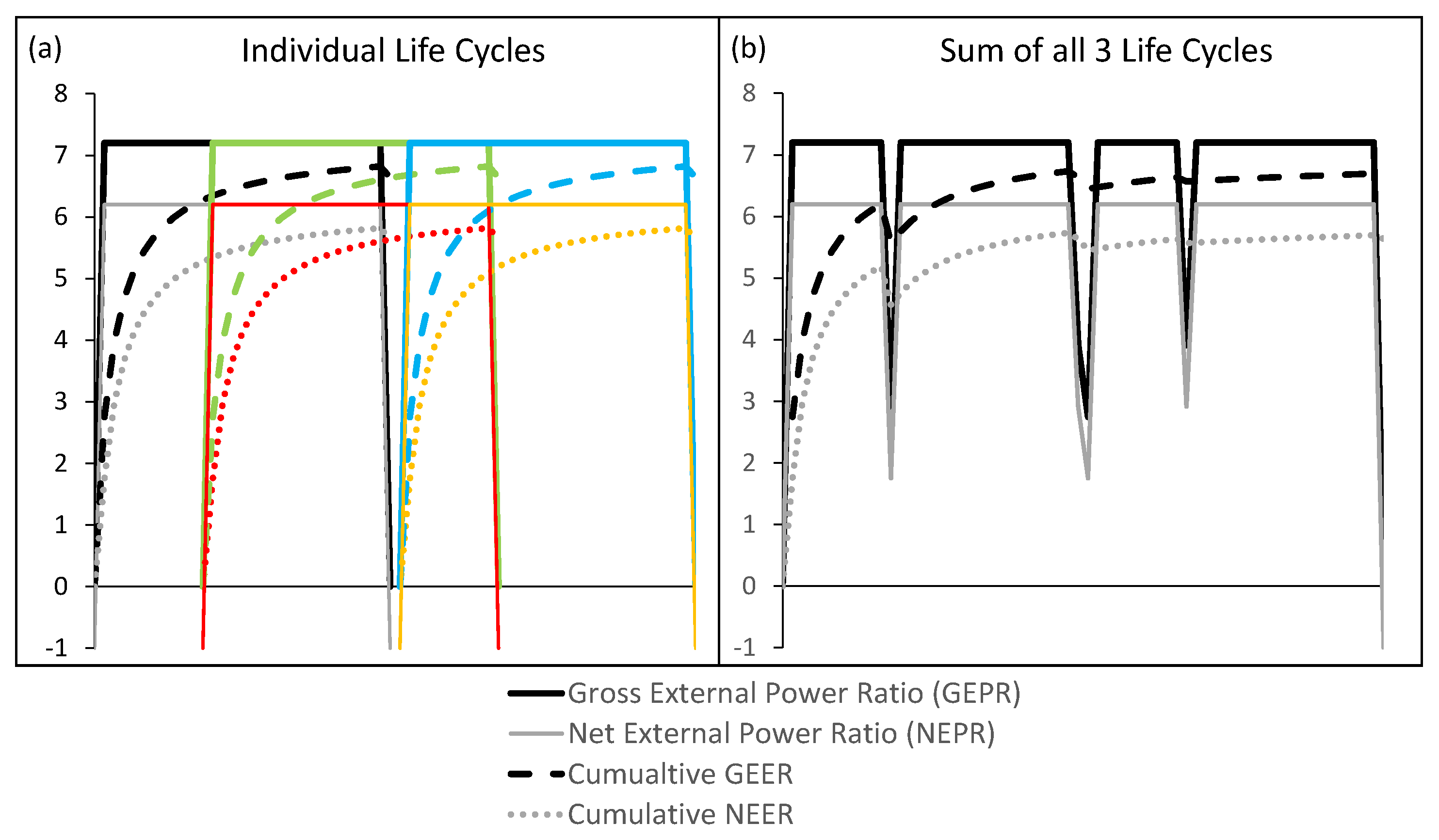
2.1. Review of Net Energy Metrics Calculated Using Full Life Cycle Energy versus Annual Energy (or Power) Flows
- ERRs and PRRs are mathematically distinct, yet not always treated as such in the net energy literature,
- distinguishing between “gross” and “net” ratios allows one to specify the difference between extraction of primary energy (gross extraction) and delivery of energy carriers to consumers (net delivered energy) without using the same term and acronym (e.g., each term has a distinct mathematical definition [29,44]) and,
- to compare ERRs and PRRs to economic metrics (e.g., to costs and prices, respectively), it is important that we understand which metrics to use for comparison (discussed in Section 4.1).


| Gross output | Net output | |||
|---|---|---|---|---|
| Feedstock included as input? | No | Yes | No | Yes |
| Power Return Ratio | GEPR | GPR | NEPR | NPR |
| Energy Return Ratio | GEER | GER | NEER | NER |
| (= EROI EROI) | (= EROI EROI) | |||
2.1.1. Power Return Ratios
2.1.2. Energy Return Ratios
2.2. Energy Intensity Ratios
2.2.1. IEA Data
2.2.2. Aggregation of EIR
2.2.3. England and United Kingdom Data
3. Results
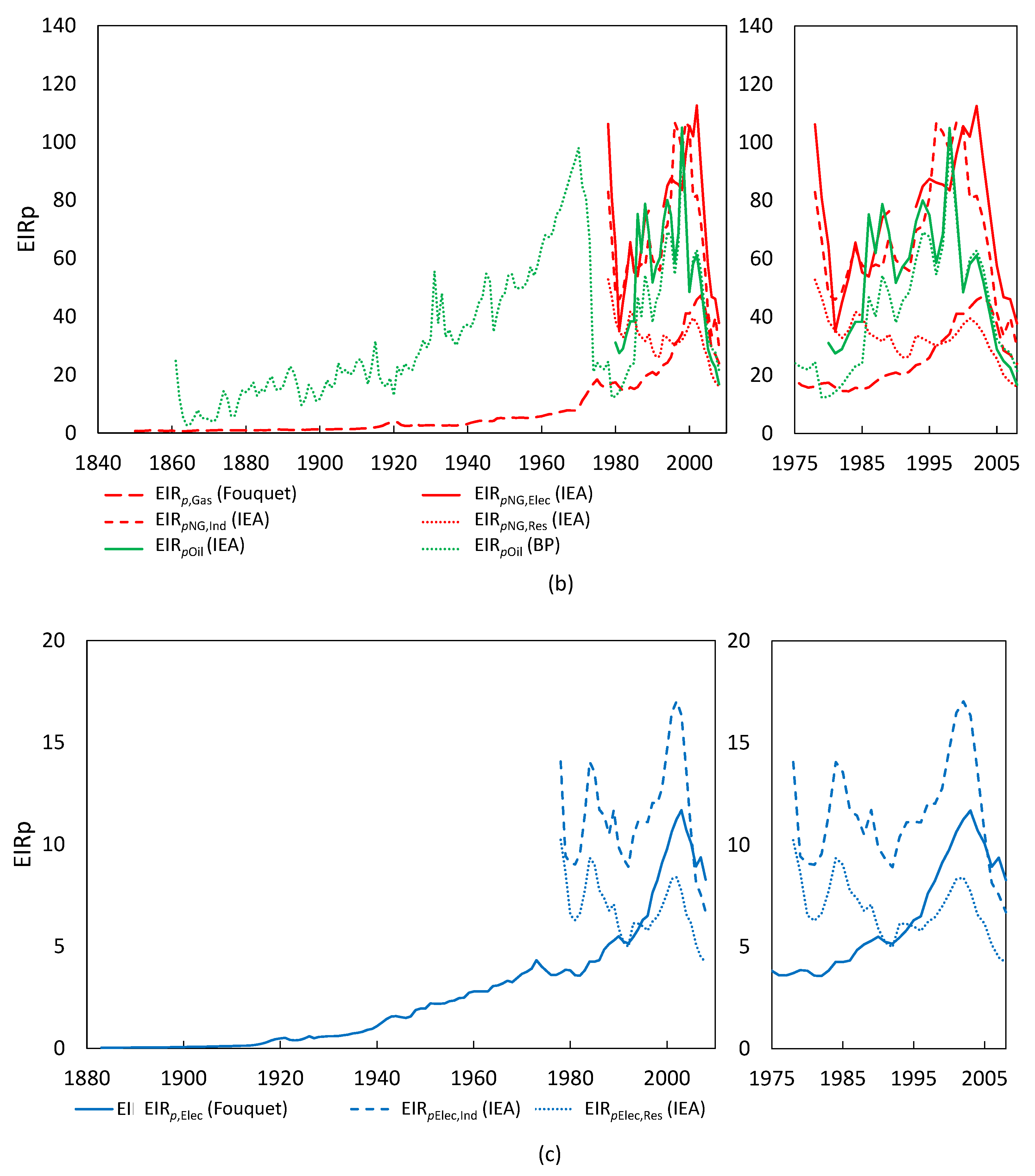
- All world average EIR follow a similar trend over the studied time periods, as they increase from 1978 to the late 1990s and early 2000s, before they decline through 2008 with a slight rebound to 2010 after the Great Recession in 2008.
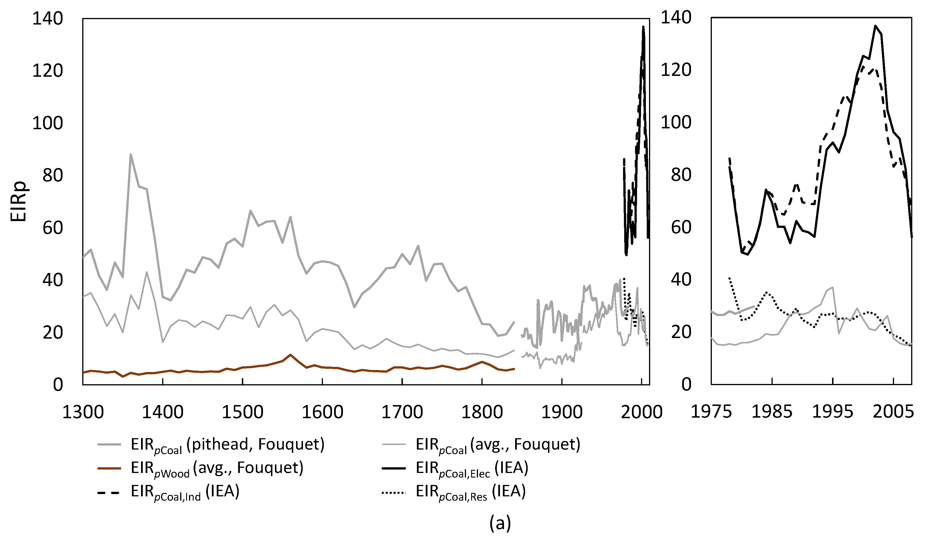
- The time series for England and the U.K. indicates that high EIR are not unprecedented before World War II, but that EIR of coal generally declined from 1300 to 1850.
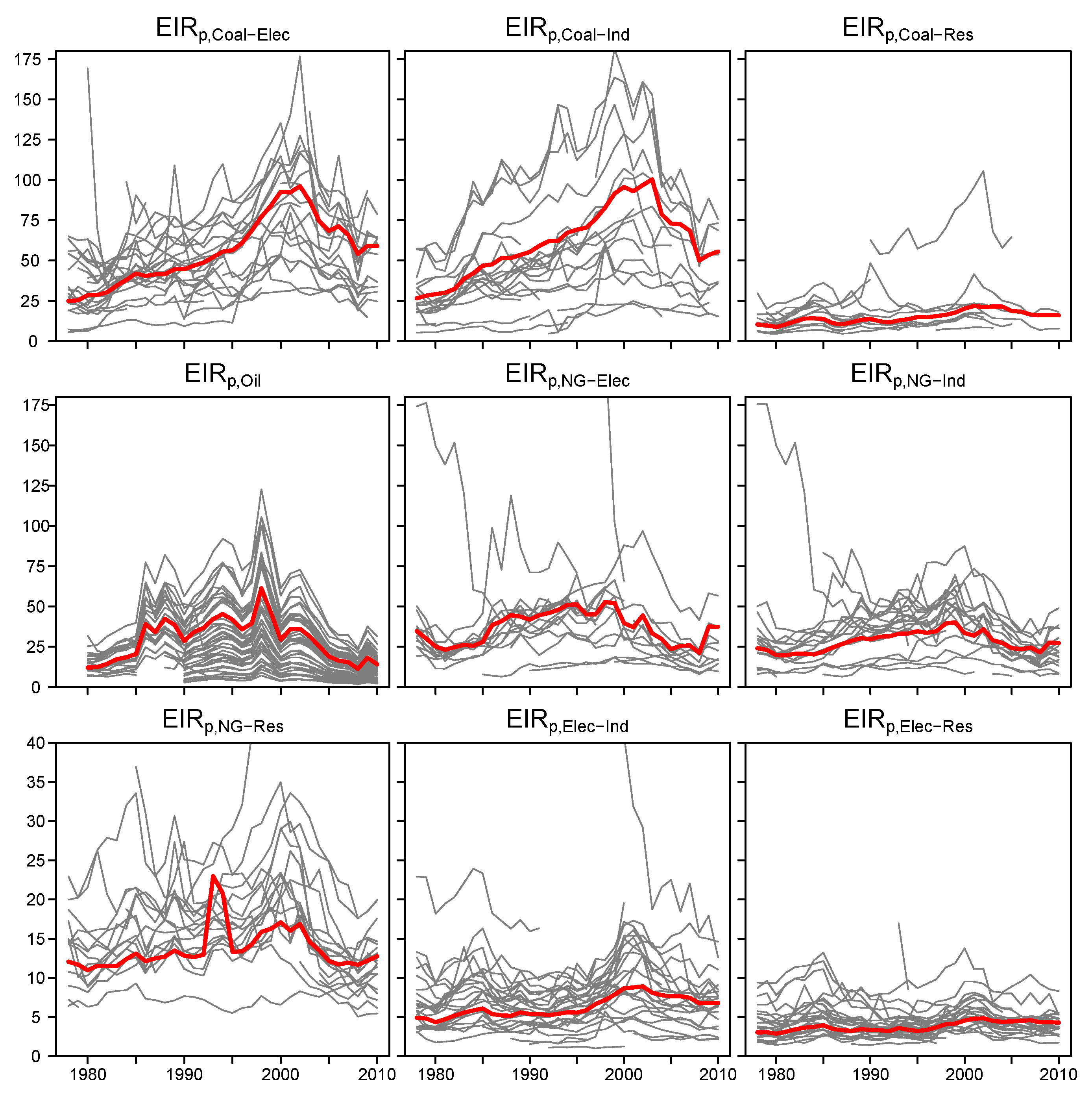
3.1. Energy Intensity Ratios: World
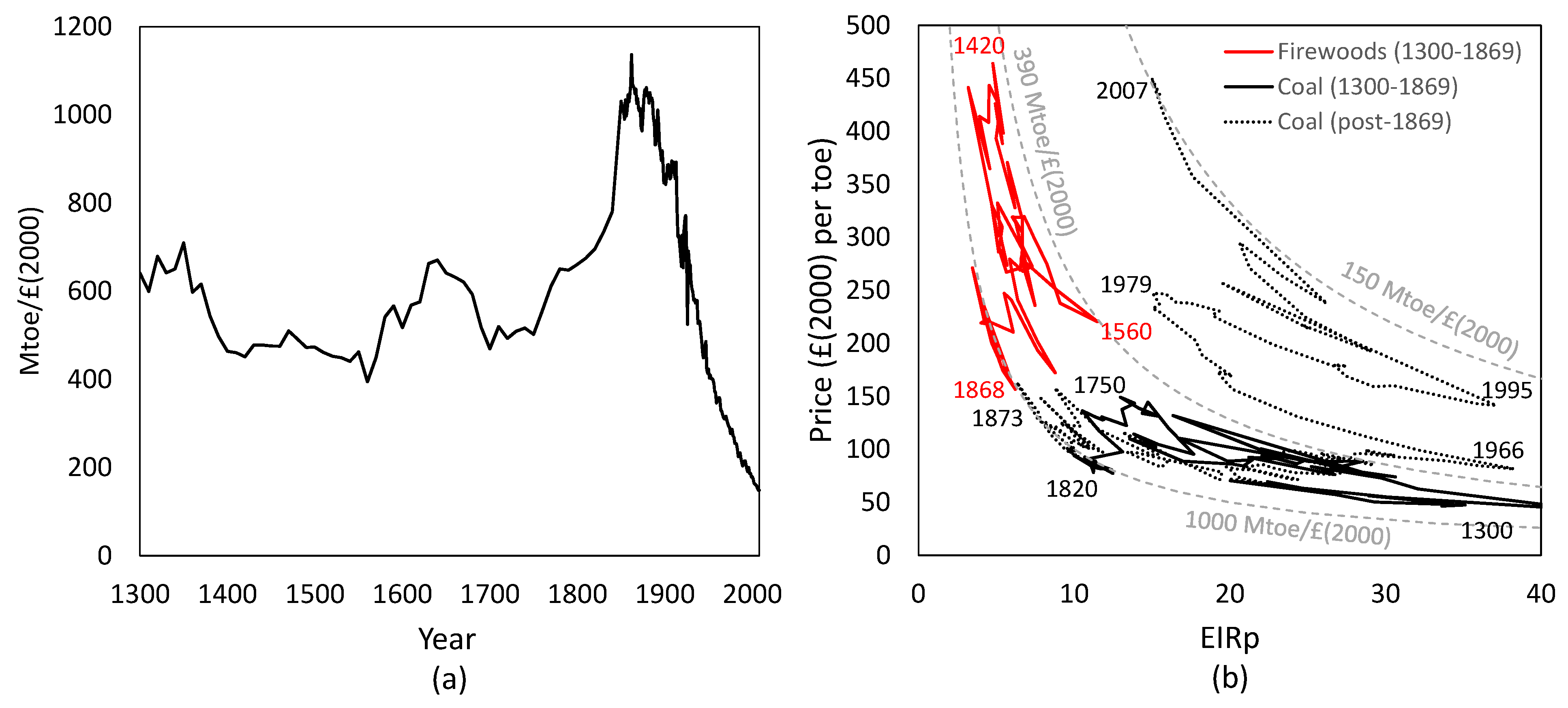
3.2. Energy Intensity Ratios: Historical England and U.K.
4. Discussion
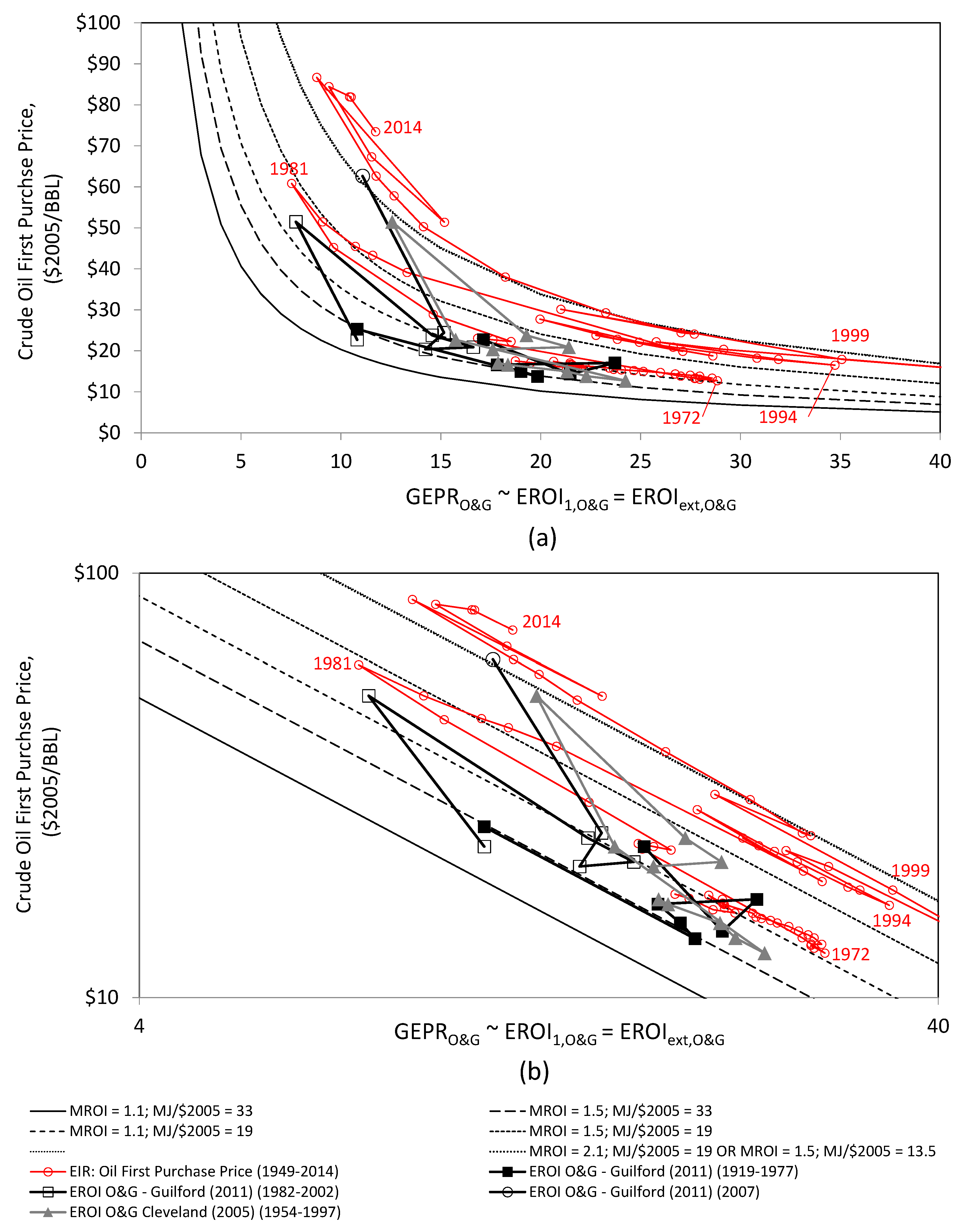
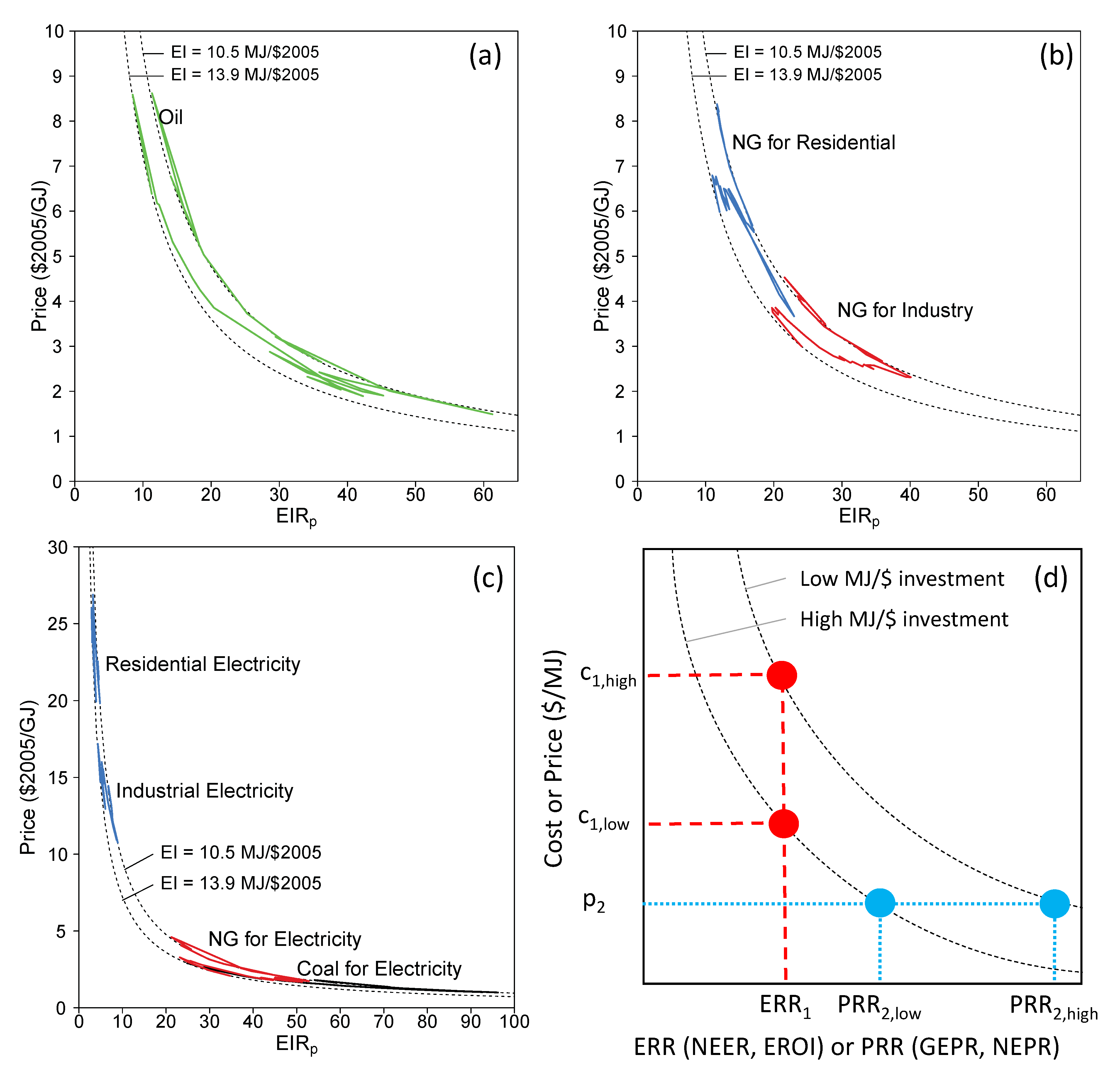
4.1. Energy and Power Return Ratios in Relation to Cost and Prices (for Future Energy Scenarios)

| EIR | EROI | EROI | EIR | EIR | EROI | |
|---|---|---|---|---|---|---|
| Year | Norway | Norway | Norway | World | World | World |
| This Paper | [63] | [63] | This Paper | This Paper | [64] | |
| 1991 | 50 | 35 | 44 | 34 | 31 | – |
| 1992 | 54 | 35 | 44 | 37 | 32 | 26 |
| 1996 | 59 | 46 | 59 | 36 | 34 | 34 |
| 1999 | 73 | 40 | 56 | 46 | 40 | 35 |
| 2006 | 29 | 26 | 47 | 16 | 23 | 18 |
| 2008 | 21 | 20 | 40 | 11 | 22 | – |
4.2. Historical England and U.K. EIR

5. Conclusions
Supplementary Files
Supplementary File 1Supplementary File 2Acknowledgments
Author Contributions
Conflicts of Interest
References
- King, C.W.; Maxwell, J.P.; Donovan, A. Comparing world economic and net energy metrics, Part 2: Expenditures Perspective. Energies 2015, 8, 12975–12996. [Google Scholar] [CrossRef]
- King, C.W. Comparing world economic and net energy metrics, Part 3: Macroeconomic Historical and Future Perspectives. Energies 2015, 8, 12997–13020. [Google Scholar] [CrossRef]
- Solow, R. A Contribution to the Theory of Economic-Growth. Q. J. Econ. 1956, 70, 65–94. [Google Scholar] [CrossRef]
- Hamilton, J. Historical Oil Shocks. In Routledge Handbook of Major Events in Economic History; Parker, R.E., Whaples, R.M., Eds.; Routledge: New York, NY, USA, 2013; p. 239265. [Google Scholar]
- Ayres, R.; Voudouris, V. The economic growth enigma: Capital, labour and useful energy? Energy Policy 2014, 64, 16–28. [Google Scholar] [CrossRef]
- Kander, A.; Stern, D.I. Economic growth and the transition from traditional to modern energy in Sweden. Energy Econ. 2014, 46, 56–65. [Google Scholar] [CrossRef]
- Kümmel, R. The Second Law of Economics: Energy, Entropy, and the Origins of Wealth; Springer: Berlin, Germany, 2011. [Google Scholar]
- Hall, C.A.S.; Klitgaard, K.A. Energy and the Wealth of Nations: Understanding the Biophysical Economy, 1st ed.; Springer: Berlin, Germany, 2012. [Google Scholar]
- Brown, J.H.; Burnside, W.R.; Davidson, A.D.; Delong, J.R.; Dunn, W.C.; Hamilton, M.J.; Mercado-Silva, N.; Nekola, J.C.; Okie, J.G.; Woodruff, W.H.; et al. Energetic Limits to Economic Growth. BioScience 2011, 61, 19–26. [Google Scholar] [CrossRef]
- Peters, G.P.; Hertwich, E.G. CO2 embodied in international trade with implications for global climate policy. Environ. Sci. Technol. 2008, 42, 1401–1407. [Google Scholar] [CrossRef] [PubMed]
- Acemoglu, D.; Robinson, J.A. Why Nations Fail: The Origins of Power, Prosperity, and Poverty; Crown Business: New York, NY, USA, 2012. [Google Scholar]
- Rutledge, D. Estimating long-term world coal production with logit and probit transforms. Int. J. Coal Geol. 2011, 85, 23–33. [Google Scholar] [CrossRef]
- Hall, C.A.S.; Cleveland, C.J.; Kaufmann, R.K. Energy and Resource Quality: The Ecology of the Economic Process; Wiley: New York, NY, USA, 1986. [Google Scholar]
- King, C.W. Energy intensity ratios as net energy measures of United States energy production and expenditures. Environ. Res. Lett. 2010, 5, 044006. [Google Scholar] [CrossRef]
- King, C.W.; Hall, C.A.S. Relating Financial and Energy Return on Investment. Sustainability 2011, 3, 1810–1832. [Google Scholar] [CrossRef]
- Henshaw, P.F.; King, C.; Zarnikau, J. System Energy Assessment (SEA), Defining a Standard Measure of EROI for Energy Businesses as Whole Systems. Sustainability 2011, 3, 1908–1943. [Google Scholar] [CrossRef]
- Heun, M.K.; de Wit, M. Energy return on (energy) invested (EROI), oil prices, and energy transitions. Energy Policy 2011, 40, 147–158. [Google Scholar] [CrossRef]
- Brandt, A.R. Converting oil shale to liquid fuels: Energy inputs and greenhouse gas emissions of the Shell in situ conversion process. Environ. Sci. Technol. 2008, 42, 7489–7495. [Google Scholar] [CrossRef] [PubMed]
- Brandt, A.R. Converting Oil Shale to Liquid Fuels with the Alberta Taciuk Processor: Energy Inputs and Greenhouse Gas Emissions. Energy Fuels 2009, 23, 6253–6258. [Google Scholar] [CrossRef]
- Brandt, A.R.; Englander, J.; Bharadwaj, S. The energy efficiency of oil sands extraction: Energy return ratios from 1970 to 2010. Energy 2013, 55, 693–702. [Google Scholar] [CrossRef]
- Guilford, M.C.; Hall, C.A.S.; O’Connor, P.; Cleveland, C.J. A New Long Term Assessment of Energy Return on Investment (EROI) for U.S. Oil and Gas Discovery and Production. Sustainability 2011, 3, 1866–1887. [Google Scholar] [CrossRef]
- Farrell, A.E.; Plevin, R.J.; Turner, B.T.; Jones, A.D.; O’Hare, M.; Kammen, D.M. Ethanol can contribute to energy and environmental goals. Science 2006, 311, 506–508. [Google Scholar] [CrossRef] [PubMed]
- Raugei, M.; Fullana-i-Palmer, P.; Fthenakis, V. The energy return on energy investment (EROI) of photovoltaics: Methodology and comparisons with fossil fuel life cycles. Energy Policy 2012, 45, 576–582. [Google Scholar] [CrossRef]
- Dale, M.; Benson, S.M. Energy Balance of the Global Photovoltaic (PV) Industry—Is the PV Industry a Net Electricity Producer? Environ. Sci. Technol. 2013, 47, 3482–3489. [Google Scholar] [CrossRef] [PubMed]
- Fthenakis, V.M.; Kim, H.C. Photovoltaics: Life-cycle analyses. Sol. Energy 2011, 85, 1609–1628. [Google Scholar] [CrossRef]
- Zhang, Y.; Colosi, L.M. Practical ambiguities during calculation of energy ratios and their impacts on life cycle assessment calculations. Energy Policy 2013, 57, 630–633. [Google Scholar] [CrossRef]
- Bullard, C.W., III; Herendeen, R.A. The energy cost of goods and services. Energy Policy 1975, 3, 268–278. [Google Scholar] [CrossRef]
- Costanza, R. Embodied Energy and Economic Valuation. Science 1980, 210, 1219–1224. [Google Scholar] [CrossRef] [PubMed]
- King, C.W. Matrix method for comparing system and individual energy return ratios when considering an energy transition. Energy 2014, 72, 254–265. [Google Scholar] [CrossRef]
- Tainter, J. The Collapse of Complex Societies; Cambridge University Press: Cambridge, UK, 1988. [Google Scholar]
- Tainter, J.A. Energy, complexity, and sustainability: A historical perspective. Environ. Innov. Soc. Transit. 2011, 1, 89–95. [Google Scholar] [CrossRef]
- Tainter, J.A. Energy and Existential Sustainability: The Role of Reserve Capacity. J. Environ. Account. Manag. 2013, 1, 213–228. [Google Scholar] [CrossRef]
- Turchin, P.; Nefedov, S.A. Secular Cycles; Princeston University Press: Princeston, NJ, USA, 2009. [Google Scholar]
- Ayres, R.U.; Warr, B. Accounting for growth: The role of physical work. Struct. Chang. Econ. Dyn. 2005, 16, 181–209. [Google Scholar] [CrossRef]
- Ayres, R.U. Sustainability economics: Where do we stand? Ecol. Econ. 2008, 67, 281–310. [Google Scholar] [CrossRef]
- Stern, D.; Kander, A. The Role of Energy in the Industrial Revolution and Modern Economic Growth; Technical Report for The Australian National University: Canberra, Australia, 2011. [Google Scholar]
- Stern, D.I.; Kander, A. The Role of Energy in the Industrial Revolution and Modern Economic Growth. Energy J. 2012, 33. [Google Scholar] [CrossRef]
- Hamilton, J. Causes and Consequences of the Oil Shock of 2007–2008. In Brookings Papers on Economic Activity; Romer, D., Wolfers, J., Eds.; Brookings Institution Press: Washington, DC, USA, 2009; p. 69. [Google Scholar]
- Hall, C.A.S.; Balogh, S.; Murphy, D.J.R. What is the Minimum EROI that a Sustainable Society Must Have? Energies 2009, 2, 25–47. [Google Scholar] [CrossRef]
- Brown, J.H.; Burger, J.R.; Burnside, W.R.; Chang, M.; Davidson, A.D.; Fristoe, T.S.; Hamilton, M.J.; Hammond, S.T.; Kodric-Brown, A.; Mercado-Silva, N.; et al. Macroecology meets macroeconomics: Resource scarcity and global sustainability. Ecol. Eng. 2014, 65, 24–32. [Google Scholar] [CrossRef] [PubMed]
- Cleveland, C.J.; Kaufmann, R.K.; Stern, D.I. Aggregation and the role of energy in the economy. Ecol. Econ. 2000, 32, 301–317. [Google Scholar] [CrossRef]
- Odum, H.T. Environmental Accounting: Energy and Environmental Decision Making; John Wiley & Sons, Inc.: New York, NY, USA, 1996. [Google Scholar]
- Campbell, D.E.; Lu, H.; Walker, H.A. Relationships among the Energy, Emergy and Money Flows of the United States from 1900 to 2011. Front. Energy Res. 2014, 2. [Google Scholar] [CrossRef]
- Brandt, A.R.; Dale, M.; Barnhart, C.J. Calculating systems-scale energy efficiency and net energy returns: A bottom-up matrix-based approach. Energy 2013, 62, 235–247. [Google Scholar] [CrossRef]
- Murphy, D.J.R.; Hall, C.A.S.; Dale, M.; Cleveland, C.J. Order from Chaos: A Preliminary Protocol for Determining EROI for fuels. Sustainability 2011, 3, 1888–1907. [Google Scholar] [CrossRef]
- Spath, P.L.; Mann, M.K.; Kerr, D.R. Life Cycle Assessment of Coal-fired Power Production, NREL/TP-570-25119; Technical Report NREL/TP-570-25119; National Renewable Energy Laboratory (NREL): Golden, CO, USA, 1999.
- Brandt, A.R.; Dale, M. A General Mathematical Framework for Calculating Systems-Scale Efficiency of Energy Extraction and Conversion: Energy Return on Investment (EROI) and Other Energy Return Ratios. Energies 2011, 4, 1211–1245. [Google Scholar] [CrossRef]
- Modahl, I.S.; Raadal, H.L.; Gagnon, L.; Bakken, T.H. How methodological issues affect the energy indicator results for different electricity generation technologies. Energy Policy 2013, 63, 283–299. [Google Scholar] [CrossRef]
- Arvesen, A.; Hertwich, E.G. More caution is needed when using life cycle assessment to determine energy return on investment (EROI). Energy Policy 2015, 76, 1–6. [Google Scholar] [CrossRef] [Green Version]
- Hall, C.A.S. Congratulations to Carey King. Environ. Res. Lett. 2012, 7, 011006. [Google Scholar] [CrossRef]
- Cleveland, C.J. Net energy from the extraction of oil and gas in the United States. Energy 2005, 30, 769–782. [Google Scholar] [CrossRef]
- Maxwell, J.P. Energy Intensity Ratios as Net Energy Measures for Selected Countries 1978–2010. Master’s Thesis, The Unversity of Texas at Austin, Austin, TX, USA, 2013. [Google Scholar]
- Fouquet, R. Heat, Power, and Light: Revolutions in Energy Services; Edward Elgar Publishing Limited: Northampton, MA, USA, 2008. [Google Scholar]
- Fouquet, R. Divergences in Long-Run Trends in the Prices of Energy and Energy Services. Rev. Environ. Econ. Policy 2011, 5, 196–218. [Google Scholar] [CrossRef]
- Fouquet, R. Long run demand for energy services: Income and price elasticities over 200 years. Rev. Environ. Econ. Policy 2014, 8. [Google Scholar] [CrossRef]
- Mitchell, T. Carbon Democracy: Political Power in the Age of Oil; Verso: London, UK; New York, NY, USA, 2013; p. 292. [Google Scholar]
- Kilian, L. Oil Price Shocks, Monetary Policy and Stagflation. CEPR Discussion Papers 7324. Available online: http://www.rba.gov.au/publications/confs/2009/kilian.html (accessed on 3 March 2015).
- Broadberry, S.; Campbell, B.; Klein, A.; Overton, M.; van Leeuwen, B. British Economic Growth, 1270–1870: An Output-Based Approach; Studies in Economics, School of Economics, University of Kent: Canterbury, Kent, UK, 2012. [Google Scholar]
- Costanza, R.; Herendeen, R.A. Embodied energy and economic value in the United States economy: 1963, 1967, and 1972. Resour. Energy 1984, 6, 129–163. [Google Scholar] [CrossRef]
- Congress of USA. Federal Nonnuclear Energy Research and Development Act, (PL 93-577); Congress of USA: Washington, DC, USA, 1974.
- Bullard, C.W.; Penner, P.S.; Pilati, D.A. Net energy analysis: Handbook for combining process and input-output analysis. Resour. Energy 1978, 1, 267–313. [Google Scholar] [CrossRef]
- Yergin, D. The Prize: The Epic Quest for Oil, Money, & Power; Free Press: New York, NY, USA, 1991; p. 928. [Google Scholar]
- Grandell, L.; Hall, C.A.; Höök, M. Energy Return on Investment for Norwegian Oil and Gas from 1991 to 2008. Sustainability 2011, 3, 2050–2070. [Google Scholar] [CrossRef]
- Gagnon, N.; Hall, C.A.S.; Brinker, L. A preliminary investigation of energy return on energy investment for global oil and gas production. Energies 2009, 2, 490–530. [Google Scholar] [CrossRef]
- Clark, G. The Long March of History: Farm Laborers Wages in England 1208–1850. NA Econ. 2001, 1, 1–35. Available online: http://www.najecon.org/naj/cache/625018000000000238.pdf (accessed on 3 March 2015). [Google Scholar]
© 2015 by the authors; licensee MDPI, Basel, Switzerland. This article is an open access article distributed under the terms and conditions of the Creative Commons by Attribution (CC-BY) license (http://creativecommons.org/licenses/by/4.0/).
Share and Cite
King, C.W.; Maxwell, J.P.; Donovan, A. Comparing World Economic and Net Energy Metrics, Part 1: Single Technology and Commodity Perspective. Energies 2015, 8, 12949-12974. https://doi.org/10.3390/en81112346
King CW, Maxwell JP, Donovan A. Comparing World Economic and Net Energy Metrics, Part 1: Single Technology and Commodity Perspective. Energies. 2015; 8(11):12949-12974. https://doi.org/10.3390/en81112346
Chicago/Turabian StyleKing, Carey W., John P. Maxwell, and Alyssa Donovan. 2015. "Comparing World Economic and Net Energy Metrics, Part 1: Single Technology and Commodity Perspective" Energies 8, no. 11: 12949-12974. https://doi.org/10.3390/en81112346
APA StyleKing, C. W., Maxwell, J. P., & Donovan, A. (2015). Comparing World Economic and Net Energy Metrics, Part 1: Single Technology and Commodity Perspective. Energies, 8(11), 12949-12974. https://doi.org/10.3390/en81112346