Investigation of High-Efficiency Wireless Power Transfer Criteria of Resonantly-Coupled Loops and Dipoles through Analysis of the Figure of Merit

Abstract

The efficiency of a Wireless Power Transfer (WPT) system is greatly dependent on both the geometry and operating frequency of the transmitting and receiving structures. By using Coupled Mode Theory (CMT), the figure of merit is calculated for resonantly-coupled loop and dipole systems. An in-depth analysis of the figure of merit is performed with respect to the key geometric parameters of the loops and dipoles, along with the resonant frequency, in order to identify the key relationships leading to high-efficiency WPT. For systems consisting of two identical single-turn loops, it is shown that the choice of both the loop radius and resonant frequency are essential in achieving high-efficiency WPT. For the dipole geometries studied, it is shown that the choice of length is largely irrelevant and that as a result of their capacitive nature, low-MHz frequency dipoles are able to produce significantly higher figures of merit than those of the loops considered. The results of the figure of merit analysis are used to propose and subsequently compare two mid-range loop and dipole WPT systems of equal size and operating frequency, where it is shown that the dipole system is able to achieve higher efficiencies than the loop system of the distance range examined.

1. Introduction

Wireless power transfer (WPT) via near-field, resonant coupling is a technology that is beginning to emerge in a range of electronic products and devices, such as charging mats and sleeves for compatible smartphones. In addition to its current electronic applications, WPT via electromagnetic resonance holds much promise for delivering efficient WPT solutions over mid-range distances, which are typically defined as one to several times the size of the transmitters/receivers comprising the system. The rapid decay of system efficiency with respect to transmission distance however means that even resonantly-coupled systems must be carefully designed in order to ensure that as much power as possible is transferred from the source to the desired end target. There are many factors influencing the transmission efficiency, and there have been studies that investigate the effects of frequency splitting [1,2], repeater coils [3,4], adaptive impedance matching techniques [5,6] and metamaterials [7].

Along with the operating frequency, the geometry of a system, defined as the shape and size of the transmitting and receiving structures, their relative alignment, configuration and the separation distance between them are particularly important quantities, as they influence both the strength of coupling between the transmitter and receiver and the intrinsic losses of the system. For near-field, resonant WPT, the ratio of coupling to losses is known as the “figure of merit” [8], and maximising this dimensionless quantity is one of the requirements to achieving high-efficiency, mid-range WPT.

Two of the most fundamental geometries in electromagnetic theory are loops and dipoles, which can be used to achieve WPT via resonantly-coupled magnetic or electric fields, respectively. Previous study of WPT between loops and dipoles was performed by Chen et al. [9], who presented a numerical analysis based on antenna theory involving conjugate-matched loop and dipole antennas. The influence of electrical size and ohmic losses of both the matching circuits and antenna structures on the WPT efficiency was considered. Their study concluded that loop systems generally outperformed their dipole counterparts; however, the configurations of the loops and dipole systems were not equivalent for the purpose of fair comparison. Furthermore, their study was performed at a fixed frequency of 13.56 MHz. Given that resonant frequency affects both the losses and coupling rate of a system and, therefore, its efficiency, it is desirable to allow the variation of this quantity with respect to the transfer efficiency. Poon [10] derived a general, numerical method based on the method of moments for calculating the WPT efficiency between two loops using self- and mutual admittances. Their analysis revealed that for coaxially-arranged loops, there was a specific frequency that maximised the transfer efficiency for a given loop radius and that this frequency decreased as the loop radius increased. The analysis presented here is able to extend this result by deriving a closed-form solution for this maximum efficiency frequency, which confirms the inverse proportionality to the loop radius observed by Poon, in addition to revealing that this frequency is the same for all separation distances and configurations. Hu et al. [11] numerically demonstrated via a four-dipole system that strongly-coupled electric fields could produce very high efficiencies, outperforming magnetically-coupled systems of a similar size, in contrast to the findings of Chen et al. This superior performance was the focus of their analysis, and no investigation into the variation of efficiency with respect to dipole size or separation distance was performed. Nam and Lee [12] used a combination of spherical modes and a conjugate-matched two-port network model to determine the theoretical upper bound that exists for electrically-small, near-field-coupled antennas. They used this to perform a general analysis that considered the variation in transfer efficiency with respect to different configurations and orientations between antennas emitting the lowest order spherical modes. Due to the existence of higher order modes in the close vicinity of even electrically-small objects, their analysis is invalid for separation distances less than one-tenth of a wavelength (0.1 λ). Given that these separation distances correspond to roughly one third of the total coupled mode region, a suitable Coupled Mode Theory (CMT) analysis is needed in order to fully investigate resonantly-coupled loop and dipole systems operating within such a vicinity to one another. This is particularly important when considering low frequency operation, wherein the coupled mode region could span large distances of the order of tens of metres. Furthermore, for the loops presented in this study, it is shown that loops lying just above the electrically-small limit achieve higher figures of merit than those operating below it, particularly as the separation distance is increased. Warnick et al. also presented an analysis regarding electrically-short loops and dipoles; however, their study only applied to weakly-coupled systems. The analysis presented in this paper is applicable to both strong and weakly-coupled loop and dipole systems [13].

Two of the most fundamental geometries in electromagnetic theory are loops and dipoles, which can be used to achieve WPT via resonantly-coupled magnetic or electric fields, respectively. Previous study of WPT between loops and dipoles was performed by Chen et al. [9], who presented a numerical analysis based on antenna theory involving conjugate-matched loop and dipole antennas. The influence of electrical size and ohmic losses of both the matching circuits and antenna structures on the WPT efficiency was considered. Their study concluded that loop systems generally outperformed their dipole counterparts; however, the configurations of the loops and dipole systems were not equivalent for the purpose of fair comparison. Furthermore, their study was performed at a fixed frequency of 13.56 MHz. Given that resonant frequency affects both the losses and coupling rate of a system and, therefore, its efficiency, it is desirable to allow the variation of this quantity with respect to the transfer efficiency. Poon [10] derived a general, numerical method based on the method of moments for calculating the WPT efficiency between two loops using self- and mutual admittances. Their analysis revealed that for coaxially-arranged loops, there was a specific frequency that maximised the transfer efficiency for a given loop radius and that this frequency decreased as the loop radius increased. The analysis presented here is able to extend this result by deriving a closed-form solution for this maximum efficiency frequency, which confirms the inverse proportionality to the loop radius observed by Poon, in addition to revealing that this frequency is the same for all separation distances and configurations. Hu et al. [11] numerically demonstrated via a four-dipole system that strongly-coupled electric fields could produce very high efficiencies, outperforming magnetically-coupled systems of a similar size, in contrast to the findings of Chen et al. This superior performance was the focus of their analysis, and no investigation into the variation of efficiency with respect to dipole size or separation distance was performed. Nam and Lee [12] used a combination of spherical modes and a conjugate-matched two-port network model to determine the theoretical upper bound that exists for electrically-small, near-field-coupled antennas. They used this to perform a general analysis that considered the variation in transfer efficiency with respect to different configurations and orientations between antennas emitting the lowest order spherical modes. Due to the existence of higher order modes in the close vicinity of even electrically-small objects, their analysis is invalid for separation distances less than one-tenth of a wavelength (0.1 λ). Given that these separation distances correspond to roughly one third of the total coupled mode region, a suitable Coupled Mode Theory (CMT) analysis is needed in order to fully investigate resonantly-coupled loop and dipole systems operating within such a vicinity to one another. This is particularly important when considering low frequency operation, wherein the coupled mode region could span large distances of the order of tens of metres. Furthermore, for the loops presented in this study, it is shown that loops lying just above the electrically-small limit achieve higher figures of merit than those operating below it, particularly as the separation distance is increased. Warnick et al. also presented an analysis regarding electrically-short loops and dipoles; however, their study only applied to weakly-coupled systems. The analysis presented in this paper is applicable to both strong and weakly-coupled loop and dipole systems [13].

Whilst the figure of merit has been used in the study of magnetically-coupled systems [8,14], it has not yet been employed in the study of dipoles. This paper calculates the figure of merit for equivalently configured loop and dipole systems and studies in detail the variation of this quantity with respect to resonant frequency, size and separation distance, which is achieved by performing a series of parameter sweeps involving the first two variables. The study of the figure of merit reveals novel insights into how the resonant frequency and key geometric parameters of the loops and dipoles can be manipulated to achieve high-efficiency WPT. The results of the figure of merit analysis are then used to perform a comparative analysis of a loop and dipole system of equal size and resonant frequency. Both of the proposed systems are shown to exhibit efficiencies that make them suitable for mid-range applications, with the dipole system exhibiting higher efficiencies than the loop system for the choice of resonant frequency over the distance range examined.

2. Theory

In this section, the elementary theoretical concepts behind Coupled Mode Theory (CMT) and the key equations required to derive the figure of merit for systems involving loops and dipoles are presented.

CMT formulates the efficiency of WPT in terms of the individual modes of electromagnetic energy that exist between two coupled objects. It is approximate in the sense that it treats the coupling between the two objects as a first order, linear perturbation of the uncoupled system [15]. Although an approximation, it is suitable for providing an accurate description of resonant, near-field WPT systems and is particularly useful for providing a general, theoretical framework [16]. It is noted that under steady-state, resonant conditions, it is equivalent to Circuit Theory (CT) [17]. Indeed, CT is needed to provide the physical context that is necessary for a CMT formulation of near-field WPT. For WPT systems operating at resonance, the efficiency as computed via CMT, ${\eta }_{CMT}$, is given by Equation (1) [18]:

$${\eta }_{CMT}=\frac{{\Gamma }_L{\kappa }^2}{{\Gamma }_T{({\Gamma }_R+{\Gamma }_L)}^2+({\Gamma }_R+{\Gamma }_L){\kappa }^2}$$

(1)

where ${\Gamma }_L$, ${\Gamma }_T$ and ${\Gamma }_R$ represent the decay rates associated with the output device (usually represented as a load connected in series with the receiver), the transmitter and the receiver, respectively. The decay rates of the transmitter, ${\Gamma }_T$, and receiver, ${\Gamma }_R$, are associated with the intrinsic losses due to Joule heating and radiation. κ denotes the coupling rate and represents how quickly the transmitter and receiver exchange energy. The matched-load condition is required to ensure that the power is transferred to the output device as efficiently as possible, thus improving the overall end-to-end efficiency of the system. The matched-load condition is calculated by maximising the efficiency, ${\eta }_{ML}$, with respect to ${\Gamma }_L$ and is given by Equation (2) [18]:

$${\Gamma }_L={\Gamma }_T\sqrt{1+\frac{{\kappa }^2}{{\Gamma }_T{\Gamma }_R}}$$

(2)

Inserting the matched-load Equation (2) into Equation (1), the matched-load efficiency, ${\eta }_{ML}$, is given by Equation (3) as [18]:

$${\eta }_{ML}=\frac{\frac{{\kappa }^2}{{\Gamma }_T{\Gamma }_R}\sqrt{1+\frac{{\kappa }^2}{{\Gamma }_T{\Gamma }_R}}}{\left(1+\sqrt{1+\frac{{\kappa }^2}{{\Gamma }_T{\Gamma }_R}}\right)\frac{{\kappa }^2}{{\Gamma }_T{\Gamma }_R}+{\left(1+\sqrt{1+\frac{{\kappa }^2}{{\Gamma }_T{\Gamma }_R}}\right)}^2}$$

(3)

From inspection of Equation (3), it can be seen that the matched-load efficiency ${\eta }_{ML}$ is solely a function of the parameter $U=\kappa /\sqrt{{\Gamma }_T{\Gamma }_R}$. This is known as the “figure of merit” and was first described in [18]. Physically, this quantity describes the ratio between the rate of energy transfer from the transmitter to the receiver and the rate energy loss from the system. Systems where $U>>1$ are said to be strongly coupled, and systems where $U<<1$ are said to be weakly coupled [18]. The matched-load efficiency can be expressed in terms of the figure of merit as U in Equation (4) [18]:

$${\eta }_{ML}=\frac{U^2\sqrt{1+U^2}}{\left(1+\sqrt{1+U^2}\right)U^2+{\left(1+\sqrt{1+U^2}\right)}^2}$$

(4)

Figure 1 plots the matched-load efficiency ${\eta }_{ML}$ against the figure of merit U. As can be seen, high-efficiency WPT is achieved for large figure of merit values, U, with values in excess of 20 ($U>20$) leading to efficiencies of greater than 90%. More generally, maximisation of the figure of merit implies maximisation of the WPT efficiency under matched-load operation, and this result motivates the analysis into the figure of merit of loops and dipoles in order to determine their high-efficiency WPT criteria. Section 2.1 and Section 2.2 present the key equations required in order to formulate the figure of merit for both loop and dipole systems, and the key dependency of this quantity on the resonant frequency, size and separation distance of the loops and dipoles is made clear.

2.1. Loops

Consider two single-turn loops of identical radius a and separated by a distance d, as shown in Figure 2(a),(b). Figure 2(a) shows the coaxial arrangement and Figure 2(b) the parallel arrangement. The corresponding equivalent coaxial and parallel dipole configurations are also shown in Figure 2(a),(b), respectively. The coupling rate for the loops, ${\kappa }_m$, is related to the loop coupling coefficient, $k_m$, as given by Equation (5) [18]:

$${\kappa }_m=\frac{{\omega }_0{k}_m}{2}$$

(5)

where ${\omega }_0=2\pi f_0$ denotes the angular resonant frequency. The coupling coefficient $k_m$ is related to the mutual inductance between the loops, M, and their individual self inductances, $L_T$ and $L_R$ (since the loops are identical $L_T=L_R=L$) via Equation (6) [19]:

$$k_m=\frac{M}{L}$$

(6)

where the self-inductance can be calculated in terms of the wire radius $R_a$, loop radius a and permeability of free space ${\mu }_0$ (since the core of the loop is air) through Equation (7) [19]:

$$L={\mu }_{0}a\left(log\left(\frac{8a}{R_a}\right)-2\right)$$

(7)

Figure 1. Variation of matched-load efficiency ${\eta }_{ML}$ with respect to the figure of merit U.

Figure 1. Variation of matched-load efficiency ${\eta }_{ML}$ with respect to the figure of merit U.

Figure 2. Loop and dipole (a) coaxial and (b) parallel configurations.

Figure 2. Loop and dipole (a) coaxial and (b) parallel configurations.

Conway [20] presented a numerically-robust, general equation to calculate the mutual inductance between loops of an arbitrary configuration. For the coaxial configuration, the mutual inductance can be expressed as Equation (8):

$$M={\mu }_0\frac{a}{\alpha }\left(\left(2-{\alpha }^2\right)K\left(\alpha \right)-2E\left(\alpha \right)\right)$$

(8)

where $\alpha =4a^2/(4a^2+d^2)$ and $K\left(\alpha \right)$ and $E\left(\alpha \right)$ denote the complete elliptic integrals of the first and second kind, respectively. For the non-coaxial arrangements, calculation of the mutual inductance is performed via numerical integration of [20]:

$$M=\frac{2{\mu }_0{a}^2}{\pi }\underset{0}{\overset{\pi }{\int }}\frac{cos\left(\varphi \right)K\left(\beta \right(\varphi \left)\right)}{\chi \left(\beta \right)}d\varphi$$

(9)

where $\chi \left(\varphi \right)=a\sqrt{2(1-cos(\varphi \left)\right)}$ and $\beta =2\sqrt{d\chi \left(\varphi \right)}/(d+\chi \left(\varphi \right))$. Equations (8) and (9) are valid when the wire radius of the loops $R_a$ is assumed to be thin, i.e., satisfying the relation $R_a/a\le 0.1$; hence, our analysis is applicable to systems that satisfy this criteria.

The intrinsic losses in the system can be described by the radiation resistance Equation (10) [21] and the ohmic resistance Equation (11) [18]:

$$\begin{array}{cc}\hfill R_{rad}& =\frac{{\mu }_0{\left({\omega }_{0}a\right)}^4\pi }{12\left(c^3\right)}\hfill \end{array}$$

(10)

$$\begin{array}{cc}\hfill R_{ohm}& =\sqrt{\frac{{\mu }_0{\omega }_0}{2\sigma }}\frac{a}{R_a}\hfill \end{array}$$

(11)

where σ denotes the conductivity of the material and c is the speed of light. The total loop self-resistance is equal to the sum of the radiation and ohmic resistances, and for two identical loops, the resistance is Equation (12):

$$R=R_T=R_R=R_{rad}+R_{ohm}$$

(12)

The self-resistance can be related to the CMT decay rates, Γ, in Equations (1)–(3) via Equation (13) [18]:

$$\Gamma =\frac{R}{2L}$$

(13)

The figure of merit for the loop, $U_m$, is given by Equation (14) from [18]:

$$\begin{array}{cc}\hfill U_m& =\frac{\kappa }{\Gamma }\hfill \end{array}$$

(14)

$$\begin{array}{cc}\hfill U_m({\omega }_0,a,d,R_a,\sigma )& =\frac{{\omega }_{0}M(a,d)}{R(a,{\omega }_0,R_a,\sigma )}\hfill \end{array}$$

(15)

where in Equation (14), the dependence of the figure of merit $U_m$ on the key parameters of loop radius a, separation distance d and resonant frequency $f_0={\omega }_0/\left(2\pi \right)$ has been made explicit. The parameter a is particularly important, as increasing this value both increases the losses in Equations (10) and (11) and the coupling via the mutual inductances (8) and (9). For this reason, the key geometric parameter of the loop is defined as its radius, a.

Alternatively, the figure of merit $U_m$ can be expressed in terms of the Q-factor, which describes the ratio between the energy stored by loops and the power dissipated in a given cycle. It can be related to the decay rates as [18]:

$$Q=\frac{{\omega }_0}{2\Gamma }$$

(16)

Using the expressions for the Q-factor Equation (16) and the coupling rate κ (5), the figure of merit between two identical loops can be written in terms of the coupling coefficient, $k_m$, (6) and their Q-factor, Q, as:

$$\begin{array}{cc}\hfill U_m& =\frac{{\kappa }_m}{\Gamma }\hfill \\ & =k_{m}Q\hfill \end{array}$$

(17)

Expression (17) for the figure of merit will be used in Section 3.3 to compare the coupling coefficients of the loops and dipoles for the configurations considered.

Given the closed-form solutions (10) and (11), maximisation of the figure of merit of the loops with respect to $f_0$ is performed by solving Equation (18) and keeping the loop radius a, wire radius $R_a$ and electrical conductivity σ as fixed:

$$\begin{array}{c}\hfill \frac{\partial U_m}{\partial f_0}=0\end{array}$$

(18)

from which the resonant frequency that maximises the figure of merit, $f_{0,max}$, is calculated using Maple 18 as:

$$f_{0,max}=\frac{1}{2\pi }{\left(\frac{2c^3}{a^3\pi }\sqrt{\frac{1}{2\sigma {\mu }_0}}\frac{1}{R_a}\right)}^{2/7}$$

(19)

Initial verification of Equation (19) was performed by dimensional analysis. Equation (19) is particularly useful for systems where there is a constraint on the size of the loops (to fit inside an electronic product, for example), but some variation in resonant frequency is permissible. Inspection of Equation (19) reveals that the resonant frequency that maximises the figure of merit is independent of the separation distance, d. This realisation is useful, since it implies that in order to achieve the highest efficiency possible for pre-specified loop radii, no distance-dependent tuning is required. Given the need for numerical calculation of the mutual inductances described by Equations (8) and (9), calculation of the loop radius a that maximises the figure of merit $U_m$ is performed numerically via parameter sweep in Section 3.1.

2.2. Dipoles

Having introduced the theory of WPT between two resonantly-coupled thin wire loops, this section presents the method for deriving the figure of merit between resonantly-coupled dipoles. Figure 2(a),(b) shows the coaxial and parallel configurations of two identical dipoles of length l, wire radius $R_a$ and separated by a distance d. The electric dipoles are also assumed to be made of thin wire and satisfy $R_a/l\le 0.1$. To obtain the coupling relationship between dipoles, the induced Electromotive Force (EMF) method is used to calculate the mutual impedance $Z_m$. This was performed using the MATLAB imped function found in [22] (p. 1011), which uses 16-point Gauss-Legendre numerical integration to calculate the mutual impedance between two dipoles by specifying their length and separation distance, with both quantities normalised with respect to the operating wavelength. In [17], it was shown that CMT is equivalent to CT under steady-state, resonant conditions and that it is possible to express the CMT equations in terms of CT variables. Using the analysis presented by both Bou [17] and Awai et al. [23], it is possible to express the figure of merit of an arbitrarily-coupled system in terms of a mutual impedance $Z_m$ existing between a coupled transmitter and receiver and their equivalent loss resistances, $R_T$ and $R_R$, respectively, as:

$$U=\frac{|Z_m|}{\sqrt{R_T{R}_R}}$$

(20)

Derivation of Equation (20) allows the figure of merit between resonantly-coupled dipoles to be calculated. In contrast to the loop system, the coupling between the dipoles is via their electric fields and, as such, represents capacitive coupling, with $Z_m<0$. For very electrically-large dipoles, the coupling mechanism can be inductive ($Z_m>0$); however, analysis at such high frequency operation is ill suited to the joint CMT-CT approach taken here. Furthermore, such systems are unsuitable for near-field WPT, since they radiate virtually all of their power into free space rather than directing it to the receiver, leading to poor system efficiencies. For two identical dipoles, $R_T=R_R=R$, and Equation (20) simplifies to $U= |Z_m|/R$. As with the loops, the losses in the dipole are due to both radiation and Joule heating and can be represented by the equivalent lumped resistances (21) [24] (p.176) and Equation (22) [18], respectively,

$$\begin{array}{cc}\hfill R_{rad}& =20{\pi }^2{\left(\frac{l}{{\lambda }_0}\right)}^2\hfill \end{array}$$

(21)

$$\begin{array}{cc}\hfill R_{ohm}& =\sqrt{\frac{{\mu }_0{\omega }_0}{2\sigma }}\frac{l}{2\pi R_a}\hfill \end{array}$$

(22)

Since the calculation of the mutual impedance between the dipoles is performed numerically, a parameter sweep is performed in order to explore the variation of the figure of merit and, therefore, also the matched-load efficiency with respect to resonant frequency and dipole length. Given the capacitive nature of the dipoles, however, initial insight into the relationship between resonant frequency and efficiency can be obtained via consideration of the figure of merit, $U_e$. By treating the coupling between the dipoles in terms of a mutual capacitance, $C_m$, and using Equation (20), the figure of merit for the dipoles can be written as Equation (23),

$$U_e=\frac{1}{{\omega }_0{C}_{m}R}$$

(23)

As is the case with mutual inductance, the mutual capacitance between two objects is solely a function of the geometry of the system. For the electric dipole system under study, this implies that the mutual capacitance is a function of dipole length l, wire radius $R_a$ and separation distance d i.e., $C_m=C_m(l,d,R_a)$. Taking this into account and considering Equations (21) and (22), which make up the loss resistance R, the figure of merit $U_e$ for the dipoles can be expressed in terms of its independent variables as Equation (24):

$$U_e({\omega }_0,l,d,R_a)=\frac{1}{{\omega }_0{C}_m(l,R_a)R({\omega }_0,l,R_a)}$$

(24)

Using the equation for the Q-factor, Q, Equation (16) introduced in Section 2.1, the figure of merit between identical dipoles Equation (23) can be equivalently defined as:

$$U_e=k_{e}Q$$

(25)

where $k_e$ describes the coupling coefficient between the dipoles, analogous to the coupling coefficient for the loops $k_m$ Equation (6), and is defined assuming capacitive coupling of the dipoles as Equation (27),

$$\begin{array}{cc}\hfill k_e& =\frac{Z_m}{Z}\hfill \end{array}$$

(26)

$$\begin{array}{cc}& =\frac{C}{C_m}\hfill \end{array}$$

(27)

The definition of the coupling coefficient, $k_e$, allows the strength of coupling existing between two identical dipoles to be compared to the strength of coupling that exists between two identical loops, as described by $k_m$ Equation (6), with this part of the analysis performed in Section 3.3.

It is immediately apparent from Equations (21), (22) and (24) that $U_e$ is inversely proportional to the resonant frequency, ${\omega }_0$. This behaviour is characteristically different from the loop system for which there was a specific resonant frequency that maximised the efficiency (with all other variables fixed). Since the losses for each system (characterised by R) are both proportional to resonant frequency, the reason for the difference in behaviour can be attributed to the fundamental difference between capacitive impedance ($\propto 1/\left({\omega }_{0}C\right)$) and inductive impedance ($\propto {\omega }_{0}L$) that couple the dipoles and loops, respectively. While the relationship between efficiency and resonant frequency for the dipoles has been identified via the figure of merit, the relationship between the efficiency and geometry of the dipole system (i.e., length, configuration and separation distance) is yet to be found. For similar reasoning of the definition of the key geometric parameter of the loops being the loop radius, a, the key geometric parameter of the dipoles is selected to be its length, l. Given the numerical approach used to determine the coupling between the dipoles, exploring the variation of the figure of merit with respect to the key geometric parameter l is performed numerically via parameter sweep, akin to the loop system, in Section 3.2.

3. Results

This section presents the results of the parameter sweeps involving the figure of merit of the loops and dipoles. The key relationships existing between the figure of merit, resonant frequency and geometric parameters of each system are identified and explained, leading to a new understanding of how high-efficiency WPT between loops and dipoles can be achieved.

3.1. Loops

The figure of merit analysis for the loop system is achieved by parameter sweeping the figure of merit, $U_m$, with respect to the resonant frequency, $f_0$, and loop radius, a, over the range Equations (28) and (29), respectively,

$$\begin{array}{c}\hfill 1\le f_0\le 150\text{MHz}\end{array}$$

(28)

$$\begin{array}{c}\hfill 0.025\le a\le 0.25\text{m}\end{array}$$

(29)

In each sweep, the loop radius a was incremented in 5-mm intervals and the resonant frequency in 1 MHz intervals. Both the conductivity and wire radius were fixed at $\sigma =6\times {10}^7$ S/m and $R_a=1$ mm, respectively. The parameter sweeps were performed over the distance range Equation (30), in 0.1 m increments (totalling five sweeps per configuration):

$$0.01\le d\le 0.5\text{m}$$

(30)

The range of resonant frequencies (28) was kept in the MHz range, specifically from 1–150 MHz, since this window both contains the frequencies typically employed in mid-range WPT systems (1–20 MHz) [1,7,8,25], as well as a number of frequencies beyond this range for further exploration. To ensure a broad enough range of interest, the choice of loop radii (29) spanned a range that was suitable for the typical applications of mid-range WPT, such as for implementation within consumer electronics products at the lower end of the range and for automotive applications toward the upper end [26,27]. It is noted that whilst the quasi-static approximation has been shown to be accurate in the study of mid-range WPT [18], combinations of resonant frequency and loop radii near the upper bounds would benefit from further analysis to determine the impact of the radiative effects and wavelike nature of the current along the loops introduced under these conditions.

Table 1 shows the value of the maximum figure of merit, $U_{m,max}$, that was achieved for each parameter sweep performed for the loop system. The accompanying loop radii, $a=a_{max}$, and resonant frequencies, $f_0=f_{0,max}$, at which each of the maximum figures of merit occurred are also shown. For both configurations, $U_{m,max}$ decreases with increasing separation distance. For distances of $d=0.1$ m and above, $a_{max}$ = 0.25 m, which corresponded to the upper bound of the loop radii range considered in Equation (29). In order to determine whether this recurrence was simply due to the limited range of loop radii considered, the upper bound of the range (29) was extended to several metres, and the parameter sweeps for both configurations were repeated for the relevant distances (d = 0.1–0.5 m). The results of the extended range parameter sweeps are also shown in Table 1. As the separation distance increases, $a_{max}$ increases to just under 4 m for both configurations at d = 0.5 m. The extended range parameter sweeps of the coaxial configuration show the largest relative increase in $U_{m,max}$, from 3.76–95 at d = 0.5 m. However, given the unsuitability of such large loops for mid-range applications, achieving the maximum figure of merit beyond “contactless” distances ($d\ge$ 0.01 m) will be unlikely.

The data in Table 1 also show that the resonant frequency $f_{0,max}$ decreases as the loop radius $a_{max}$ increases. This result is in keeping with Equation (19), which is plotted in Figure 3(a) with respect to the loop radius a. In order to provide further validation of Equation (19), values of $f_{0,max}$ were randomly selected from each of the parameter sweeps for a given radius, a, and are also plotted in Figure 3(a). The agreement between the $f_{0,max}$ predicted by Equation (19) and the corresponding values obtained from the randomly-sampled parameter sweeps is clear. The invariance of $f_{0,max}$ with respect to separation distance according to Equation (19) is also supported by the results of the parameter sweeps. This agreement can be noticed by observing that the only change in $f_{0,max}$ in Table 1 occurs when there is a change in $a_{max}$.

Given the inverse relationship between $f_{0,max}$ and a, it is interesting to consider the subsequent variation in the electrical size of the loops, $S_{0,max}$, defined as Equation (31),

$$S_{0,max}={\beta }_{0,max}a$$

(31)

where ${\beta }_{0,max}=2\pi f_{0,max}/c$, $c=3\times {10}^8$ m/s (free space speed of light). Figure 3(b) plots $S_{0,max}$ with respect to a over the unextended range (29). It can be seen from the Figure that the ideal combinations of resonant frequency $f_{0,max}$ and loop radius a for high-efficiency WPT lie above the electrically-small limit $S_{0,max}\le 0.1$. Therefore, given the overall observed increase in $a_{max}$ with respect d, loops of larger electrical size will be required for ensuring that the maximum WPT efficiency is achieved.

Table 1. Maximum figure of merit values, $U_{m,max}$, for the parameter sweeps of the loop system. The loop radii, $a_{max}$, and resonant frequencies, $f_{0,max}$, corresponding to each maximum are also given.

	d (m)	0.01	0.1	0.2	0.3	0.4	0.5
Coaxial	$U_{m,max}$	510	155	77.0	43.7	26	16.3
	$a_{max}$ (m)	0.09	0.25	0.25	0.25	0.25	0.25
	$f_{0,max}$ (MHz)	71	30	30	30	30	30
Coaxial (extended range)	$U_{m,max}$	-	190	141	119	104	95
	$a_{max}$ (m)	-	0.9	1.98	2.62	2.73	3.76
	$f_{0,max}$ (MHz)	-	10	5	4	4	3
Parallel	$U_{m,max}$	47.1	14.4	7.42	4.48	2.95	2.06
	$a_{max}$ (m)	0.09	0.25	0.25	0.25	0.25	0.25
	$f_{0,max}$ (MHz)	71	30	30	30	30	30
Parallel (extended range)	$U_{m,max}$	-	17.6	13.0	10.96	9.68	8.80
	$a_{max}$ (m)	-	0.8	1.62	2.57	3.57	3.71
	$f_{0,max}$ (MHz)	-	11	6	4	3	3

Table 1. Maximum figure of merit values, $U_{m,max}$, for the parameter sweeps of the loop system. The loop radii, $a_{max}$, and resonant frequencies, $f_{0,max}$, corresponding to each maximum are also given.

	d (m)	0.01	0.1	0.2	0.3	0.4	0.5
Coaxial	$U_{m,max}$	510	155	77.0	43.7	26	16.3
	$a_{max}$ (m)	0.09	0.25	0.25	0.25	0.25	0.25
	$f_{0,max}$ (MHz)	71	30	30	30	30	30
Coaxial (extended range)	$U_{m,max}$	-	190	141	119	104	95
	$a_{max}$ (m)	-	0.9	1.98	2.62	2.73	3.76
	$f_{0,max}$ (MHz)	-	10	5	4	4	3
Parallel	$U_{m,max}$	47.1	14.4	7.42	4.48	2.95	2.06
	$a_{max}$ (m)	0.09	0.25	0.25	0.25	0.25	0.25
	$f_{0,max}$ (MHz)	71	30	30	30	30	30
Parallel (extended range)	$U_{m,max}$	-	17.6	13.0	10.96	9.68	8.80
	$a_{max}$ (m)	-	0.8	1.62	2.57	3.57	3.71
	$f_{0,max}$ (MHz)	-	11	6	4	3	3

Figure 3. Variation of (a) the maximum efficiency resonant frequency $f_{0,max}$ with respect to the loop radius a and (b) the variation in the electrical size of the loop $S_{0,max}$ when operating at $f_{0,max}$ with respect to loop radius a.

Figure 3. Variation of (a) the maximum efficiency resonant frequency $f_{0,max}$ with respect to the loop radius a and (b) the variation in the electrical size of the loop $S_{0,max}$ when operating at $f_{0,max}$ with respect to loop radius a.

Table 1 also shows the values of $U_{m,max}$ for the coaxial configuration exceed the corresponding values for the parallel arrangement. More generally, for a given loop radius, resonant frequency and separation distance, the coaxial configuration produces a higher figure of merit than the parallel configuration. This can be seen by simply comparing the colour bars in Figure 4(a),(b),(c) and Figure 5(a),(b),(c), which show the results of the parameter sweeps at d = 0.01, 0.1 and 0.5 m for each loop configuration. Although the superiority of the coaxial configuration over the parallel configuration is not a new realisation, the figure of merit analysis shows that careful selection of resonant frequency and loop radius can still lead to reasonably efficient WPT (almost 40% at $d=0.5$ m when $U_m\approx U_{m,max}=2.06$) for loops arranged in the parallel configuration. Given that this configuration is widely overlooked in the literature, the feasibility of WPT using this arrangement has not been demonstrated before.

Figure 4. Variation of the figure of merit $U_m$ for the loop system with respect to resonant frequency $f_0$ and loop radius a for (a) $d=0.01$ m, (b) $d=0.1$ m and (c) $d=0.5$ m for the coaxial configuration.

Figure 4. Variation of the figure of merit $U_m$ for the loop system with respect to resonant frequency $f_0$ and loop radius a for (a) $d=0.01$ m, (b) $d=0.1$ m and (c) $d=0.5$ m for the coaxial configuration.

Figure 5. Variation of the figure of merit $U_m$ for the loop system with respect to resonant frequency $f_0$ and loop radius a for (a) $d=0.01$ m, (b) $d=0.1$ m and (c) $d=0.5$ m for the parallel configuration.

Figure 5. Variation of the figure of merit $U_m$ for the loop system with respect to resonant frequency $f_0$ and loop radius a for (a) $d=0.01$ m, (b) $d=0.1$ m and (c) $d=0.5$ m for the parallel configuration.

Closer inspection of Figure 4(a) and Figure 5(a) show that there is a large red band, denoting figures of merit that are within approximately 20% of $U_{m,max}$. There is also a reduction in the size of this high figure of merit area as the separation distance increases. As such, operating as close to $f_{0,max}$ and $a_{max}$ becomes increasingly important as the separation distance is increased. This reduction implies that as the separation distance increases, the number of resonant frequencies and loop radii that combine to produce the near-maximum figures of merit decreases, and this reduction is present for both configurations.

3.2. Dipoles

In order to fairly compare the figure of merit of the dipole system to that of the loop system, the parameter sweeps involving the dipoles were performed over the same frequency range Equation (28) and for the same separation distances Equation (30). The wire radius and conductivity of the dipole were similarly fixed at $R_a=1$ mm and $\sigma =6\times {10}^7$ S/m, respectively. In order to ensure that the analysis considered dipoles of similar sizes to the loops, the dipole length l was set equal to the diameter of the loops, so that $l=2a$. Given this condition and the range of loop radii Equation (29), the range of lengths l in each parameter sweep corresponded to Equation (32):

$$0.05\le l\le 0.5$$

(32)

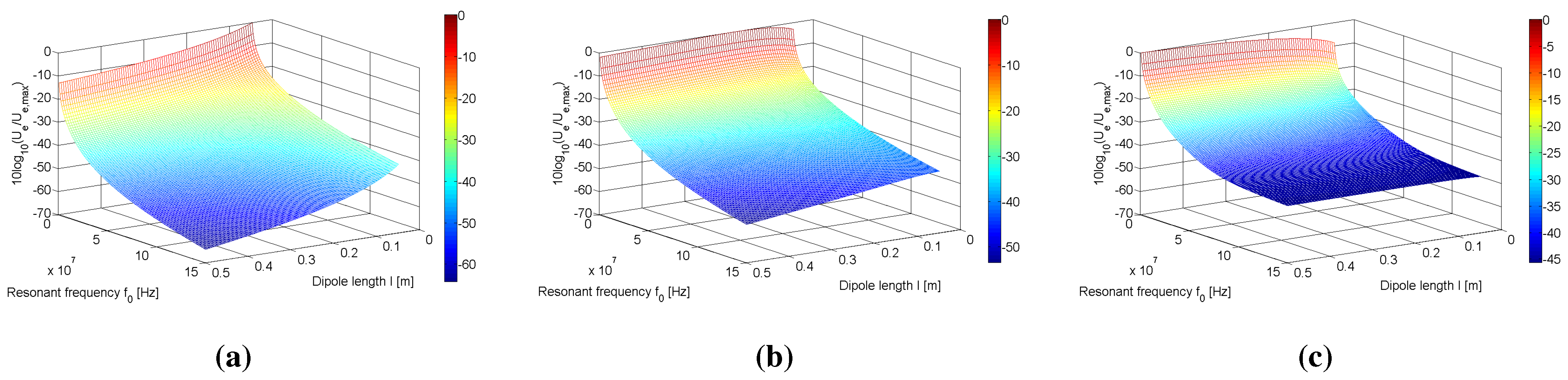
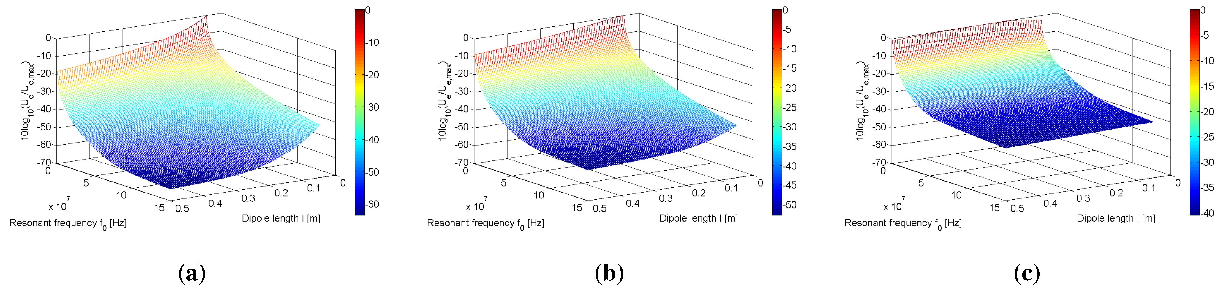
Figure 6(a)–(c) and Figure 7(a)–(c) show the results of the parameter sweeps for each configuration d = 0.01, 0.1 and 0.5 m. Table 2 lists the maximum figures of merit, $U_{e,max}$, obtained for each of the parameter sweeps, along with the dipole length $l_{max}$ and resonant frequencies $f_{0,max}$ for which they occurred. As the resonant frequency was increased from $f_0=1$ MHz (corresponding to lowest resonant frequency of the range considered), a rapid decrease in the figure of merit was observed, in keeping with Equation (23). It was therefore necessary in Figure 6(a)–(c) and Figure 7(a)–(c) to normalise the figure of merit according to Equation (33) in order to allow visual interpretation of the results,

$$U_{e,norm}=10lo{g}_{10}\left(\frac{U_e}{U_{e,max}}\right)$$

(33)

The normalisation expressed by Equation (33) represents the relative loss in the figure of merit with respect to the maximum value, $U_{e,max}$, of each of the parameter sweeps. In each of the sweeps, $U_{e,max}$ occurred at the lower bound of the frequency range in Equation (28) (1 MHz).

Figure 6(a) and Figure 7(a) show large reductions of up to 40 dB in the figure of merit of both configurations as the resonant frequency is increased from $f_0=1$ MHz to $f_0=150$ MHz. Given that the figure of merit for the coaxial and parallel configurations are of the order 10${}^4$ and 10${}^5$, respectively, at $d=0.01$ m and $l=0.5$ m, a drop of 40 dB from this value produces figures of merit of the orders of 10${}^0$ and 10${}^1$, respectively. This exponential decrease drops the practically 100% efficiencies of both configurations to approximately 17% and 82%, respectively, having a more adverse effect on the coaxial configuration in this instance. When coupled with the overall decrease in the maximum figure of merit, $U_{e,max}$, with respect to increasing separation distance (see Table 2), low frequency operation for larger separation distances becomes increasingly important.

The reductions in the figure of merit with respect to operating at lengths outside $l_{max}$ are less severe than what is observed for operating at frequencies outside of $f_{0,max}$. Reductions of almost 20 dB across the range of frequencies are still possible, however. Whilst unimportant for low frequency operation (≤10 MHz), the resulting decrease in efficiency for dipoles of length $l\ne l_{max}$ at high resonant frequencies (≥150 MHz) is significant. For example, at $d=0.1$ m, $f_0=150$ MHz and $l=l_{max}=0.18$ m, the figure of merit $U_e=87$, corresponding to an efficiency of 97%. Changing the dipole length in this instance to $l=0.5\text{m}\ne l_{max}$, the figure of merit drops by approximately 15 dB, resulting in an efficiency of 49%. This reduction amounts to an almost 50% decrease in efficiency. Therefore, it can be concluded that operating the dipoles at $l=l_{max}$ is necessary when the figure of merit becomes sufficiently low, due to large separation distance and/or high frequency operation of the dipoles.

Figure 6. Variation of the figure of merit $U_m$ for the dipole system with respect to resonant frequency $f_0$ and dipole length l for (a) $d=0.01$ m, (b) $d=0.1$ m and (c) $d=0.5$ m for the coaxial configuration.

Figure 6. Variation of the figure of merit $U_m$ for the dipole system with respect to resonant frequency $f_0$ and dipole length l for (a) $d=0.01$ m, (b) $d=0.1$ m and (c) $d=0.5$ m for the coaxial configuration.

Figure 7. Variation of the figure of merit $U_e$ for the dipole system with respect to resonant frequency $f_0$ and dipole length l for (a) $d=0.01$ m, (b) $d=0.1$ m and (c) $d=0.5$ m for the parallel configuration.

Figure 7. Variation of the figure of merit $U_e$ for the dipole system with respect to resonant frequency $f_0$ and dipole length l for (a) $d=0.01$ m, (b) $d=0.1$ m and (c) $d=0.5$ m for the parallel configuration.

Comparing the maximum figures of merit of the dipole contained within Table 2 to the corresponding loop values in Table 1, it is immediately apparent that the dipole system achieves figures of merit that are roughly three to four orders of magnitude higher than the loops. In contrast to the loops, where the coaxial configuration produced the higher figures of merit, the parallel dipole configuration offers the greatest $U_{e,max}$. Table 2 also shows an increase in $l_{max}$ as the distance between the dipoles increases, similarly observed for $a_{max}$ in Table 1. For separation distances of $d\ge 0.3$ m, Table 2 shows $l_{max}=0.5$ m for the parallel configuration. Since these lengths corresponded to the upper bound of the dipole length range Equation (32), the upper bound of Equation (32) was increased and the parameter sweeps re-run, revealing that for d = 0.3, 0.4 and 0.5 m, $l_{max}\ge 0.5$. However, given that $U_{e,max}\ge {10}^4$ in the original parameter sweeps, the moderate increase in $U_{e,max}$ achieved by increasing the original range of l results in a negligible effect on the already near 100% efficiencies. This reinforces the fact that at low resonant frequency operation (1 MHz in this case), there is freedom in the choice of dipole length l when seeking high-efficiency WPT.

Table 2. Maximum figure of merit values, $U_{m,max}$, for the parameter sweeps of the dipole system at $d=0.1-0.5$ m for both coaxial and parallel configurations. The dipole lengths, $l_{max}$, and resonant frequencies, $f_{0,max}$, at which each maximum occurs are also provided.

	d (m)	0.01	0.1	0.2	0.3	0.4	0.5
Coaxial	$U_{e,max}$	6.48 ×10${}^6$	2.76 × 10${}^5$	6.87 × 10${}^4$	3.05 × 10${}^4$	1.17 ×10${}^4$	1.00 ×10${}^4$
	$l_{max}$ (m)	0.05	0.06	0.11	0.17	0.22	0.28
	$f_{0,max}$ (MHz)	1	1	1	1	1	1
Parallel	$U_{e,max}$	5.01 × 10${}^7$	7.56 × 10${}^5$	1.87 × 10${}^5$	8.22 × 10${}^4$	4.34 × 10${}^4$	2.53 × 10${}^4$
	$l_{max}$ (m)	0.05	0.18	0.36	0.5	0.5	0.5
	$f_{0,max}$ (MHz)	1	1	1	1	1	1
Parallel (extended range)	$U_{e,max}$	-	-	-	8.25 × 10${}^4$	4.60 × 10${}^4$	2.91 × 10${}^4$
	$l_{max}$ (m)	-	-	-	0.54	0.72	0.89
	$f_{0,max}$ (MHz)	-	-	-	1	1	1

Table 2. Maximum figure of merit values, $U_{m,max}$, for the parameter sweeps of the dipole system at $d=0.1-0.5$ m for both coaxial and parallel configurations. The dipole lengths, $l_{max}$, and resonant frequencies, $f_{0,max}$, at which each maximum occurs are also provided.

	d (m)	0.01	0.1	0.2	0.3	0.4	0.5
Coaxial	$U_{e,max}$	6.48 ×10${}^6$	2.76 × 10${}^5$	6.87 × 10${}^4$	3.05 × 10${}^4$	1.17 ×10${}^4$	1.00 ×10${}^4$
	$l_{max}$ (m)	0.05	0.06	0.11	0.17	0.22	0.28
	$f_{0,max}$ (MHz)	1	1	1	1	1	1
Parallel	$U_{e,max}$	5.01 × 10${}^7$	7.56 × 10${}^5$	1.87 × 10${}^5$	8.22 × 10${}^4$	4.34 × 10${}^4$	2.53 × 10${}^4$
	$l_{max}$ (m)	0.05	0.18	0.36	0.5	0.5	0.5
	$f_{0,max}$ (MHz)	1	1	1	1	1	1
Parallel (extended range)	$U_{e,max}$	-	-	-	8.25 × 10${}^4$	4.60 × 10${}^4$	2.91 × 10${}^4$
	$l_{max}$ (m)	-	-	-	0.54	0.72	0.89
	$f_{0,max}$ (MHz)	-	-	-	1	1	1

3.3. Coupling Coefficients and Q-Factors of Loops and Dipoles

Using the definitions for the coupling coefficients of the loops and dipoles, $k_m$ Equation (6) and $k_e$ Equation (26), respectively, it is possible to compare the relative coupling strength that exists between the two geometries when they are of a similar size, i.e., $l=2a$. By doing so, it is possible to determine the underlying mechanism that is responsible for the dipole system generating maximum figures of merit that are much greater than those produced by the loop system.

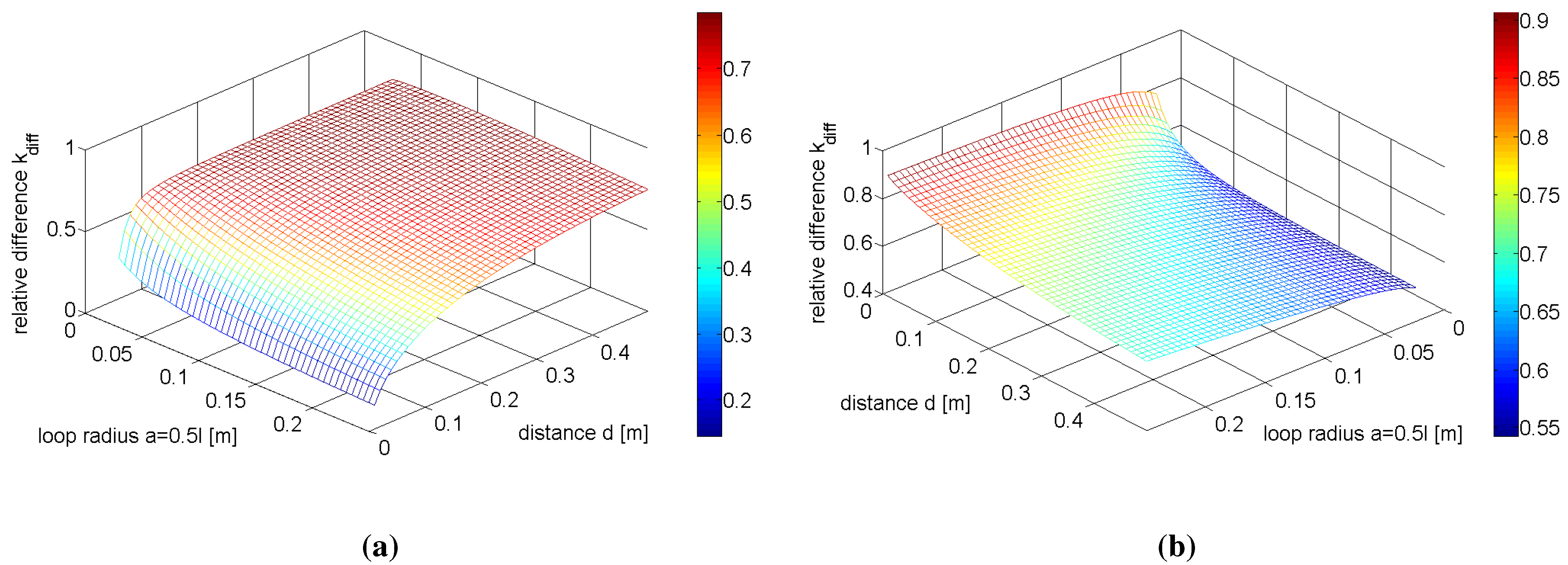
Figure 8(a),(b) plots the relative difference between the loop and dipole coupling coefficients, $k_{diff}$, described by Equation (34):

$$k_{diff}=\frac{k_m-k_e}{k_m}$$

(34)

for the ranges in Equations (28)–(30) and (32), under the condition $l=2a$. Given however that the dipole system exhibits higher figures of merit in the parallel configuration and the loop system in the coaxial configuration, it is more meaningful to calculate $k_{diff}$ between these two superior configurations, and this is shown in Figure 8(a). Similarly, the relative difference, $k_{diff}$, between the coupling coefficients of the coaxial dipole configuration and parallel loop configuration, representing the lower figure of merit configurations for each geometry, is shown in Figure 8(b).

In Figure 8(a),(b), $k_{diff}>0$, therefore showing that the coupling between the loops is stronger than that of dipoles. Figure 8(a) shows $k_{diff}$ increases as the separation distance increases, up to a maximum of roughly 0.7 at d = 0.5 m, implying that the dipole coupling coefficient decays more rapidly with respect to distance than that of the loops. The opposite is true in Figure 8(b), where $k_{diff}$ decreases with respect to increasing distance. The largest relative difference between the two coupling coefficients in Figure 8(b) occurs at a = 0.25 m and d = 0.01 m, where $k_{diff}$ = 0.9.

The main conclusion that can be drawn from the analysis into the coupling coefficients of the loop and dipole, however, is that for the range of loop radii, dipole lengths and distances considered, the higher figures of merit displayed by the dipole system in Section 3.2 do not arise as a consequence of stronger coupling in relation to the loop system. Given this result, Equations (17) and (25) introduced in Section 2.1 and Section 2.2 therefore imply that the Q-factor of the dipole is significantly higher than that of the loops. The Q-factor of the dipole, assuming capacitive behaviour, can be written as Equation (35):

$$Q_e=\frac{1}{{\omega }_{0}CR}$$

(35)

(where C represents the self-capacitance of the dipole) and the Q-factor of the loop can be written as Equation (36):

$$Q_m=\frac{{\omega }_{0}L}{R}$$

(36)

Figure 8. Relative difference $k_{diff}$ between the coupling coefficients of the loops and dipoles for (a) the parallel dipole and coaxial loop configurations and (b) the coaxial dipole and parallel loop configurations.

Figure 8. Relative difference $k_{diff}$ between the coupling coefficients of the loops and dipoles for (a) the parallel dipole and coaxial loop configurations and (b) the coaxial dipole and parallel loop configurations.

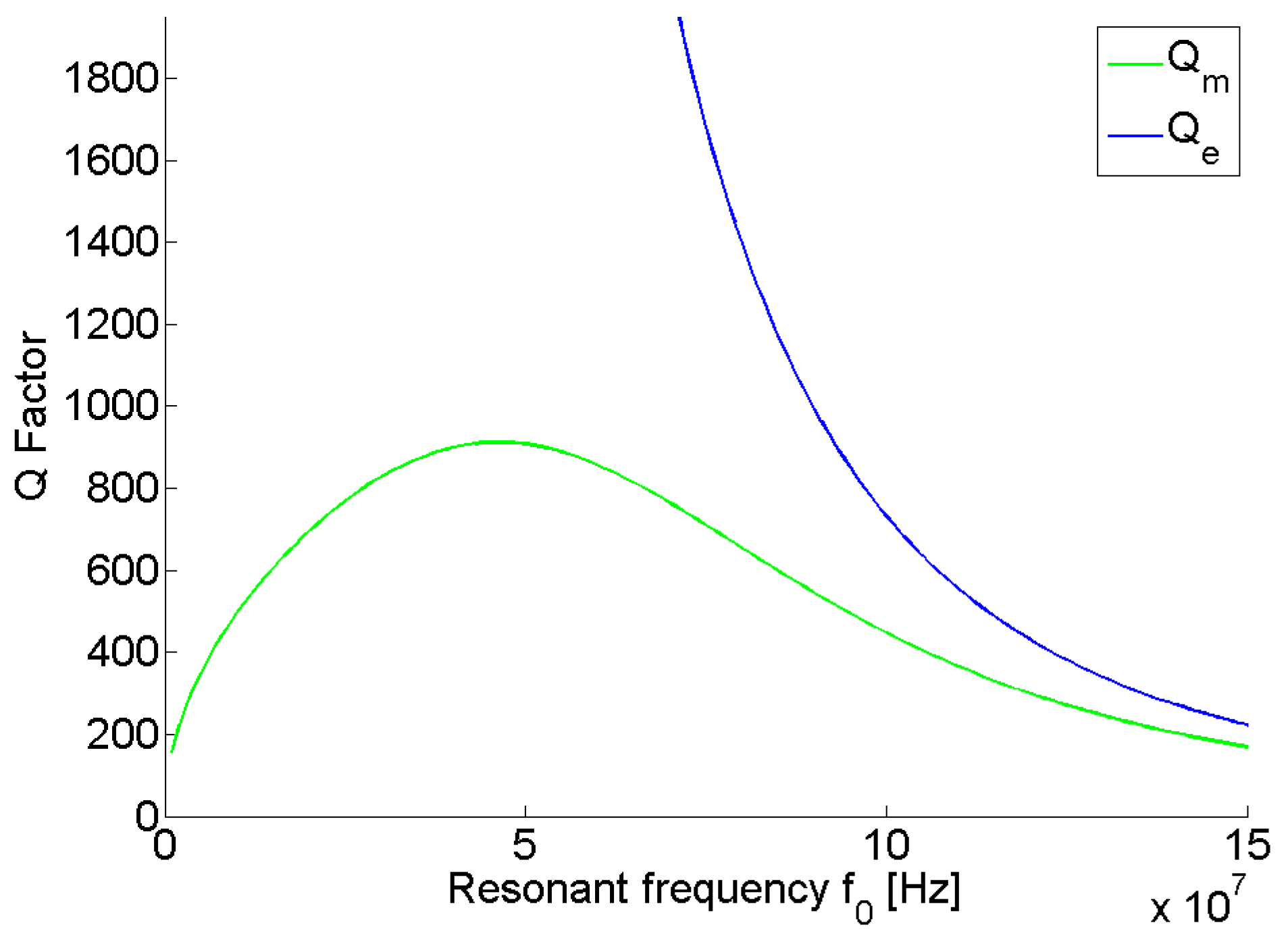
By way of example, Equations (35) and (36) are plotted in Figure 9 for l = 2a = 0.3 m for the frequency range described by Equation (28). Given that from Equations (10) and (11), $R\propto {\omega }_0$, increasing the frequency of the loops both increases the reactive power stored (through the factor ${\omega }_{0}L$ in Equation (36)) and the intrinsic losses. Therefore, the Q-factor of the loops reaches a finite maximum value, arising from the need to balance the these two factors. This relationship has also been reported for coils in [28] and has been subsequently utilised in the design of high-Q coils for state-of-the-art inductive WPT systems [29,30]. For the example case shown in Figure 9, the peak in the Q-factor occurs at 46 MHz.

For the dipole however, the Q-factor is inversely proportional to ${\omega }_0$, and, hence, theoretically $Q\to \infty$ for ${\omega }_0\to 0$. Physically, decreasing the frequency both increases the reactive power stored by the dipole due its capacitive nature and also decreases its intrinsic losses. As such, for sufficiently low frequencies, the dipoles are able to achieve significantly higher figures of merit than the loops, despite weaker coupling. These relationships explain why there is a specific resonant frequency that maximises the figure of merit of the loop system, unlike the dipole where the maximum figure of merit was obtained for the lowest possible resonant frequency. As the frequency increases, however, the Q-factor of the dipole decreases rapidly, and hence, it is therefore possible for the loop system to show superior WPT efficiency for sufficiently high resonant frequencies.

Figure 9. Variation in $Q_m$ and $Q_e$ with respect to $f_0$ for l = 2a = 0.3 m.

Figure 9. Variation in $Q_m$ and $Q_e$ with respect to $f_0$ for l = 2a = 0.3 m.

3.4. Efficiency

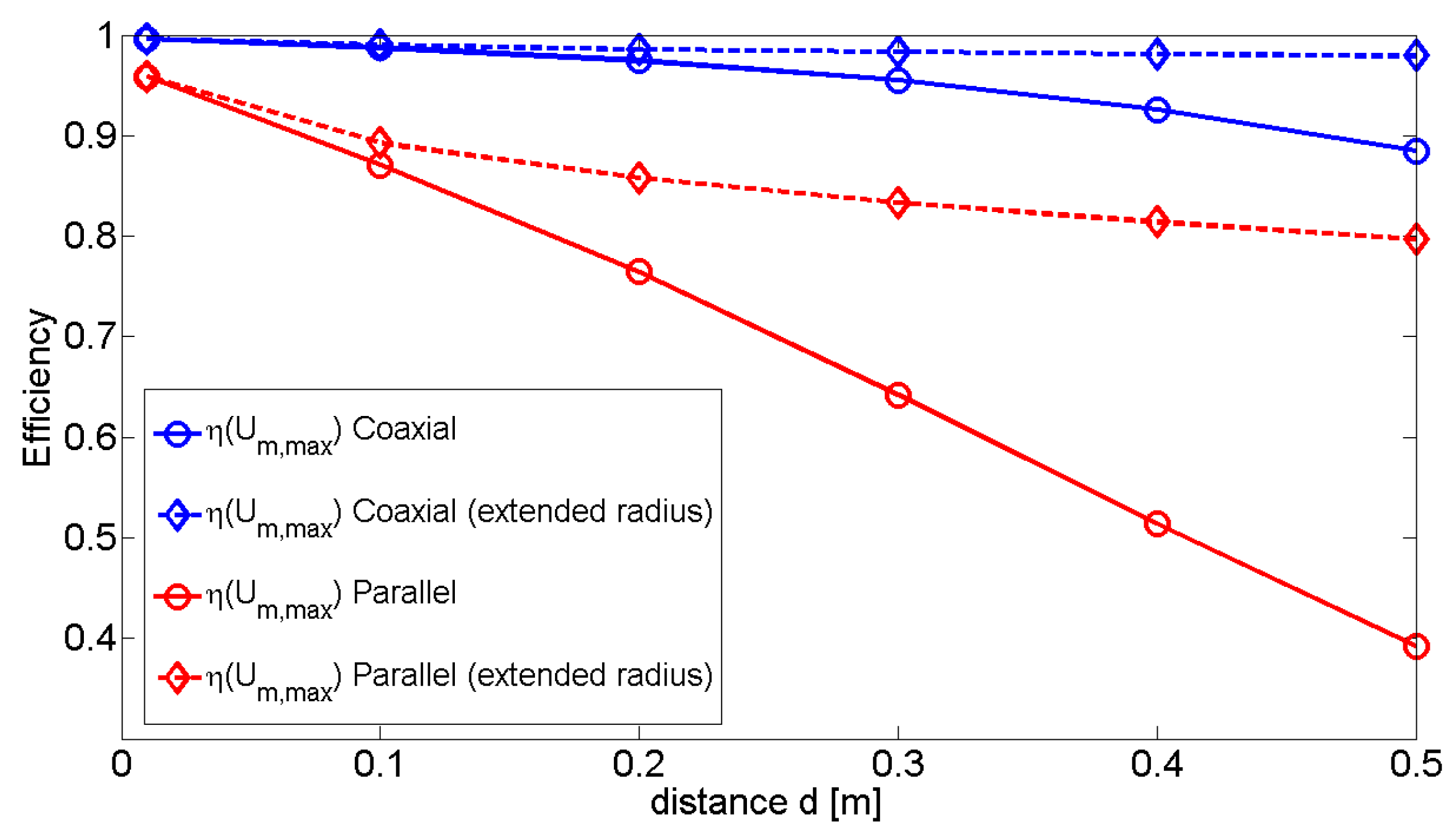
Using the data presented in Table 1, Figure 10 plots the efficiencies for each configuration of the loop system when operating at $U_{m,max}$ with respect to the separation distance. The increases achieved by operating at the correct resonant frequency and loop radius combination are visible, particularly for the parallel configuration, where a 30% increase in efficiency at d = 0.5 m can be seen. No plot of the dipole is presented as $U_{m,max}\ge {10}^4$ throughout Table 2, therefore resulting in a constant near 100% for each configuration and distance examined.

Figure 10. Efficiencies for each configuration of the loop system when operating at $U_{m,max}$. The efficiencies were computed using the data in Table 1.

Figure 10. Efficiencies for each configuration of the loop system when operating at $U_{m,max}$. The efficiencies were computed using the data in Table 1.

By using the relationships identified in Section 3.1 and Section 3.2, it is however possible to demonstrate how the higher figures of merit associated with the dipole system directly translate into higher WPT efficiencies than those produced by loop systems of a similar size. The result that it was not possible for a loop system of fixed radius to achieve the maximum figure of merit for all separation distances provided a degree of freedom in the choice of loop radius. Therefore, a loop radius of $a=0.15$ m was selected, which was deemed to be both of sufficient size to be useful for mid-range applications and large enough to produce high efficiencies over a reasonable distance range. Maintaining the same wire radius $R_a=1$ mm and conductivity $\sigma =6\times {10}^7$ S/m as were employed in the parameter sweeps, Equation (19) gives $f_{0,max}=46.1$ MHz. In order to compare the performance of the loops against a similarly-sized dipole system, the dipole length was set as $l=2a=0.3$ m. It is noted that whilst this condition realises a comparative analysis of the efficiencies in terms of geometry, different comparisons may be of more importance to other applications, e.g., form-factor, delivered power, etc.

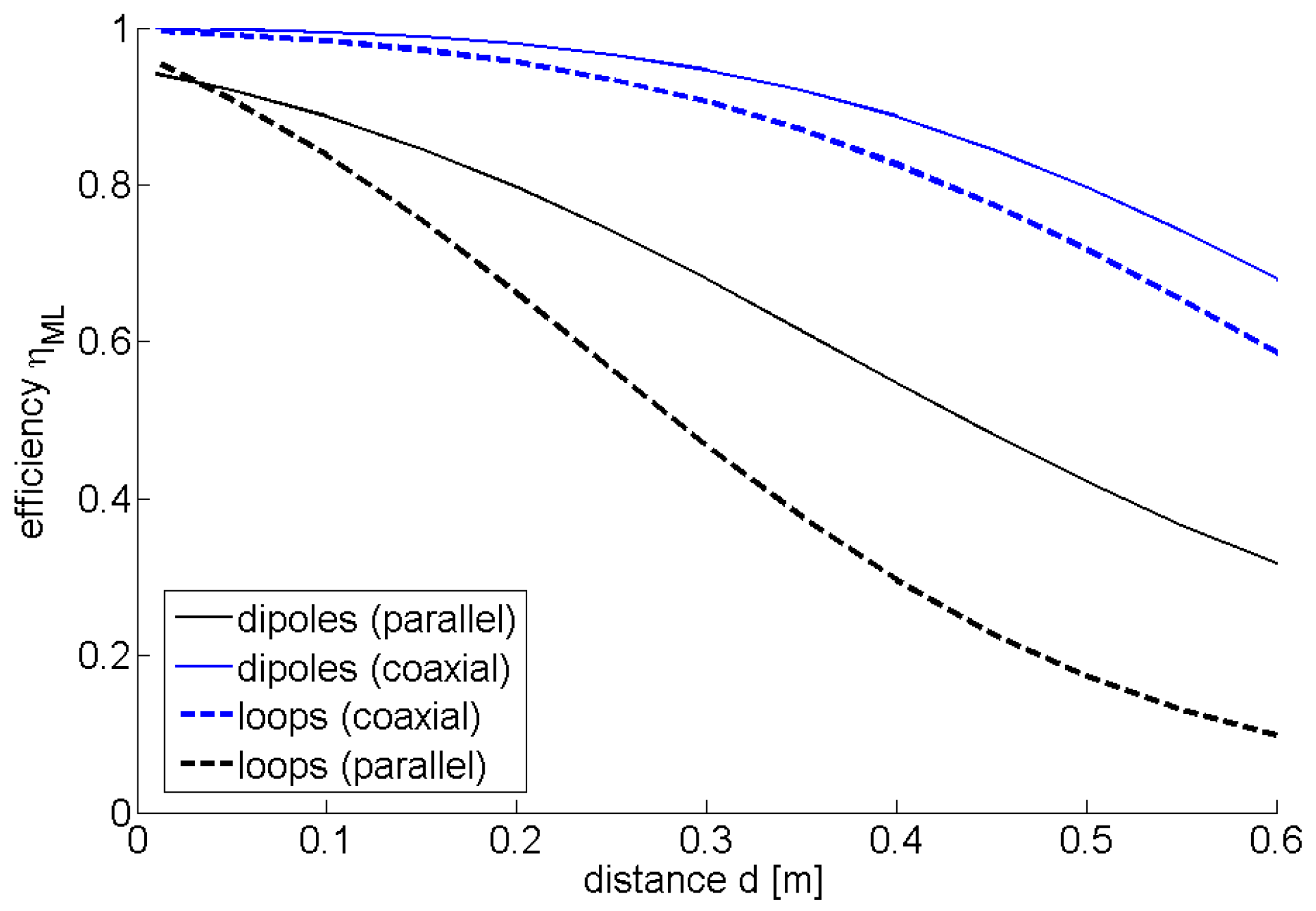
The calculated efficiencies for each configuration of the loop and dipole systems are shown in Figure 11. The efficiency was computed up to a separation distance of $d=0.6$ m, slightly beyond the distance of $d=0.5$ m explored in the parameter sweeps. The distance was extended to this value for two reasons. Firstly, it represented twice the characteristic size of the loop and dipole systems, i.e., $d=2l=4a=0.6$ m. Secondly, it was reported in [18] that the quasi-static approximation for magnetically-coupled resonance was valid for ${\omega }_{0}d/c\approx 0.5$, and since the study presented here utilises the same approximation for the loop system, the distance was restricted accordingly (${\omega }_{0}d/c=0.5781\approx 0.5$). Beyond $d=0.6$ m, further analysis would be required to determine the validity of the magneto-static approximation.

Despite operating at a resonant frequency of $f_0=46.1$ MHz, which lies significantly above $f_{0,max}$ identified in the figure of merit analysis, the dipole system exhibits higher efficiencies than the loop system. In particular, the dipole system exhibits less degradation in efficiency between the two configurations than the loop system. This is important for dynamic systems where loss in efficiency due to misalignment is to be a low as possible. Despite exhibiting the lower efficiencies of the two geometries, the results of Figure 11 show the proposed loop system to nevertheless be suitable for mid-range WPT, with efficiencies of 42% possible at $d=0.5$ m. In particular, the feasibility of reasonably-efficient WPT from loops arranged in parallel is apparent from Figure 11, which shows an efficiency of 47% possible with this configuration at $d=0.3$ m.

Figure 11. Matched-load efficiencies of the coaxial and parallel configurations of the loop and dipole systems operating at $f_0=46.1$ MHz and $l=2a=0.3$ m.

Figure 11. Matched-load efficiencies of the coaxial and parallel configurations of the loop and dipole systems operating at $f_0=46.1$ MHz and $l=2a=0.3$ m.

4. Discussion

Detailed analysis of the figure of merit has facilitated the identification of the key relationships that exist between geometry, resonant frequency and high-efficiency WPT involving pairs of resonantly-coupled, identical loops and dipoles. The analysis has been performed via a series of parameter sweeps at various mid-range distances and assuming the loop and dipoles involved were of fixed thin wire radius, $R_a$, and material conductivity, σ. Under the correct choice of resonant frequency, dipole length and loop radius, the feasibility of WPT between the two less-studied configurations of the loops (parallel) and dipoles (coaxial) has been demonstrated.

For the dipole, it has been revealed that the dominant factor in achieving large figures of merit was low frequency operation, which, if kept in the range of a few MHz, could reach figures of merit of the order ${10}^7$ and ${10}^6$. This frequency regime offered relative freedom in the choice of dipole length, as only minor reductions to the large figures of merit were experienced, maintaining the efficiency close to 100%. This result shows promise for delivering solutions in the numerous applications of mid-range WPT that constrain the size of the transmitter and receivers, such as in mobile phones and laptops, for example. However, the large figures of merit enjoyed at low frequencies decayed exponentially as the frequency increased, with drops in efficiency of up 80% experienced for the coaxially-arranged dipoles operating at $f_0=150$ MHz, dipole length $l=0.5$ m and separation distance $d=0.01$ m. For such high frequency operation, the correct choice of dipole length becomes an important factor, and significant savings in efficiency (approximately 50% in the example given in Section 3.2) are seen. Further consideration also needs to be given to the effect of the losses of the inductors used to achieve resonance in the dipoles. This was investigated by Chen et al. [9] and, so, was not repeated in this study; however, it is noted that low frequency operation of the dipoles will require larger inductances in order to achieve resonance (e.g., 244 mH for a dipole of length $l=0.3$ m operating at 1 MHz). Typically, larger inductances are associated with higher resistances due to the higher permeability cores and greater sizes required than smaller inductors, introducing additional loss and, therefore, reducing the figure of merit. Increasing the resonant frequency of the dipoles will reduce the inductance; however, higher frequency operation introduces further losses in the inductor due to the proximity and skin effects. Increasing the resonant frequency also reduces the figure of merit of the dipoles, as reported in Section 3.2. Which one of these effects dominates over the other is unclear, since other factors affecting the choice of inductor, such as power levels, have not been considered in the analysis. For the purposes of efficiency, however, it suffices to note that the choice of resonant frequency for the dipoles will be dependent on the inductors used to achieve resonance, with larger inductors with as little loss as possible being the optimal choice.

It has been confirmed that the equivalently-sized dipole system is able to achieve higher efficiencies than the loop system when operating at the same resonant frequency of $f_0=46$ MHz for distances up to $0.6$ m. Considering that the majority of the focus in the design of mid-range WPT systems is targeted towards magnetic resonance, it has been shown that high-efficiency WPT is also possible using resonantly-coupled electric fields. Additionally, the new insights presented in this study regarding magnetic resonance involving coupled loops can be used to provide improvements to WPT systems employing these objects. The key relationships identified in this study further contribute to the goal of developing high-efficiency WPT systems using electromagnetic resonance.

5. Conclusions

This paper, by calculating the figure of merit for resonantly-coupled loop and dipole systems, has explored and identified their high-efficiency WPT criteria in terms of their key geometric parameters and resonant frequency. In contrast to previous studies, which typically used antenna theory to consider WPT between loops and dipoles with respect to either geometry or resonant frequency, the formulation of the CMT figure of merit in this study has allowed concurrent analysis of both of these parameters, revealing novel relationships that can be exploited in the future design of WPT systems involving resonantly-coupled loops and dipoles.