Real-Time Estimation of Power System Frequency Using a Three-Level Discrete Fourier Transform Method

Abstract

This paper proposes a three-level discrete Fourier transform (DFT) method to provide an accurate estimate of power system frequency in real time. The first level decomposes a power system signal into two orthogonal cosine- and sine-filtered signals. The second and third levels are used to determine the amplitude ratio of the cosine- and sine-filtered signals without encountering the zero-crossing problem and with an increase in ability to suppress harmonics and inter-harmonics. The performance of the three-level DFT method is evaluated using computer-simulated signals with harmonics and inter-harmonics. The three-level DFT method is also implemented on a digital signal processor (DSP)-based hardware prototype, and its performance in the hardware implementation is evaluated using a real-time digital simulator (RTDS). The evaluation results show that the three-level DFT method can achieve real-time estimation of power system frequency with satisfactory performance.

1. Introduction

The frequency is one of the most important quantities in the operation of power systems, and its deviation is a good indicator of abnormal operating conditions. Therefore, estimation of the power system frequency is an important task in the monitoring, protection and control of power systems. In particular, accurate estimation of the power system frequency in real time is a prerequisite for rapid-response applications, including load shedding, generator protection, and renewable energy control [1,2,3]. Although the power system frequency may deviate from the nominal value due to unexpected system disturbances, the transient response of rapid-response applications should be no longer than four to five power system frequency cycles [1].

The zero-crossing method is one of the simplest ways to estimate the power system frequency, and involves measuring the time interval between consecutive zero crossings of a power system signal [4]. However, measured signals in real power systems typically contain harmonic distortions, which may introduce significant errors when using the zero-crossing method. To address with this problem, a variety of approaches have been proposed over the past couple of decades, including orthogonal [1,5,6,7,8,9,10,11,12,13], modified zero-crossing [6,14], phase-locked loop [15,16,17], Kalman filtering [18,19,20,21], adaptive filtering [22,23,24,25,26], least error square [21,27,28,29,30,31,32], neural network [33,34], Newton-algorithm [35,36,37,38], Prony [1,10], and wavelet approaches [39,40,41]. Orthogonal approaches have attracted widespread attention for real-time use, due to their estimation accuracy and ease of implementation. Demodulation methods [5,6,7], finite impulse response (FIR) filter-based methods [1,8,9,10], and discrete Fourier transform (DFT)-based methods [11,12,13] are orthogonal approaches. Although these methods suppress harmonics and inter-harmonics effectively, most of them have certain limitations. In exceptional cases, some methods, such as those described in [12,13], can increase their ability to suppress harmonics at the cost of ease of implementation. When greater ability to suppress harmonics is required, the implementations increase in complexity and it becomes more difficult to complete real-time estimation of the power system frequency within the required DSP timer-interrupt interval. Consequently, depending on the required ability level, these methods can become impractical for real-time applications.

In this paper we propose a three-level DFT method for real-time and accurate estimation of the power system frequency. Triple use of DFTs allows accurate frequency estimation with a particular increase in ability to suppress harmonics and inter-harmonics. Although the three-level DFT method leads to an additional two-cycle delay compared with other DFT-based orthogonal approaches, it is fast enough for rapid-response applications where the delay should be no more than five cycles in total. Evaluation results confirm the efficiency and validity of the three-level DFT method to achieve real-time estimation of the power system frequency.

The remainder of this paper is organized as follows: frequency estimation using the three-level DFT method is formulated in Section 2, and the performance is evaluated in Section 3 using both computer simulations and a digital signal processor (DSP)-based hardware implementation. Conclusions are drawn in Section 4.

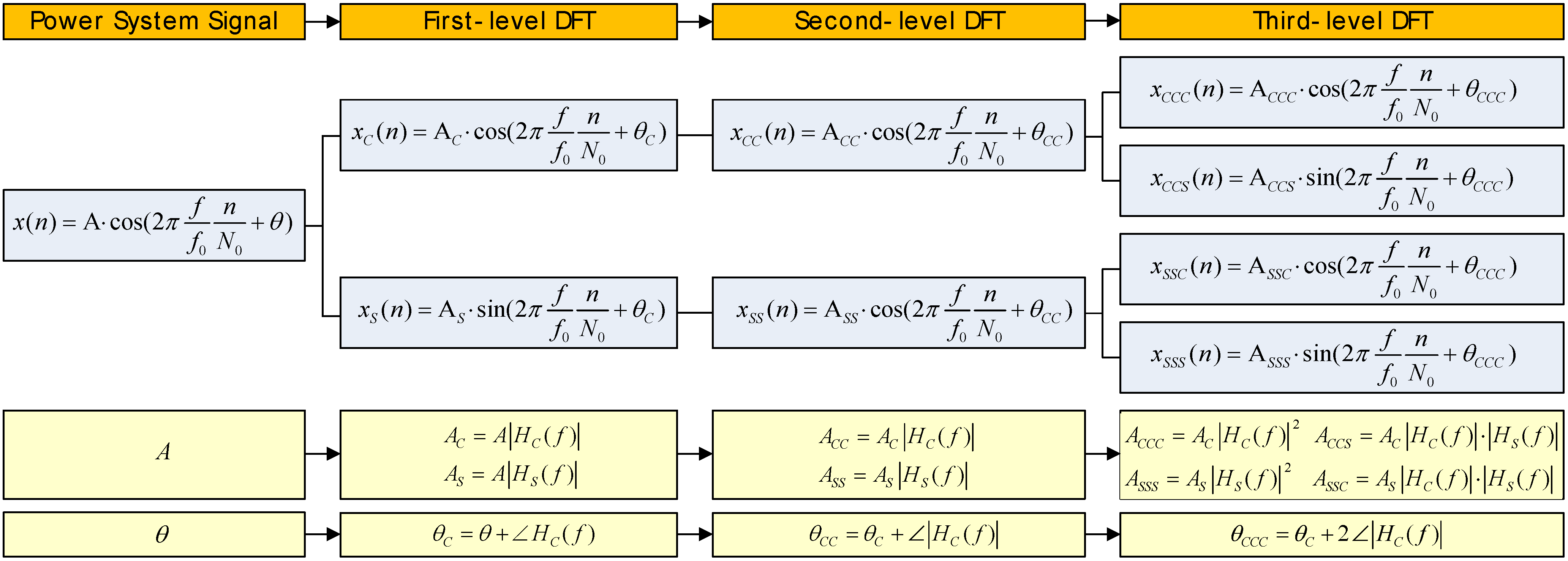
2. Frequency Estimation

Assuming that a power system signal has a purely sinusoidal waveform with an amplitude $A$ , power system frequency f, and phase θ, it can be described in discrete time steps as:

$$x(n)=A\cdot \text{cos}(2\text{π}\frac{f}{f_0}\frac{n}{N_0}+\text{θ})$$

(1)

where f₀ is the nominal frequency and N₀ is the number of samples per cycle at f₀. The power system signal can be decomposed into two orthogonal signals via DFT, using cosine and sine filters. The coefficients of the cosine filter in the DFT are:

$$H_C(n)=\frac{2}{N_0}\text{cos}(2\text{π}\frac{n}{N_0}+\frac{\text{π}}{N_0})\hspace{1em}\hspace{1em}n=0,\hspace{0.17em}\dots ,\hspace{0.17em}{N}_0-1$$

(2)

The amplitude and phase response of the cosine filter can be found from the unilateral Z-transform of Equation (2):

$$|H_C(f)|=\frac{4}{N_0}\cdot \frac{\text{cos}(\frac{\text{π}}{N_0})\text{sin}(\frac{\text{π}}{N_0}\frac{f}{f_0})\text{sin}(\text{π}\frac{f}{f_0})}{\text{cos}(\frac{2\text{π}}{N_0}\frac{f}{f_0})-\text{cos}(\frac{2\text{π}}{N_0})}$$

(3)

$$\angle H_C(f)=\text{π}-\text{π}\frac{N_0-1}{N_0}\frac{f}{f_0}$$

(4)

Applying Equations (3) and (4) to $x(n)$ in Equation (1) yields a cosine-filtered signal of the first-level DFT:

$$x_C(n)=A_C\cdot \text{cos}(2\text{π}\frac{f}{f_0}\frac{n}{N_0}+{\text{θ}}_C)$$

(5)

where AC = A|H_C(f)| and ${\text{θ}}_C=\text{θ}+\angle H_C(f)$. Note that A_C and θ_C depend on the power system frequency. Similarly, the coefficients of the sine filter in the DFT are:

$$H_S(n)=-\frac{2}{N_0}\text{sin}(\frac{2\text{π}}{N_0}n+\frac{\text{π}}{N_0})\hspace{1em}\hspace{1em}n=0,\hspace{0.17em}\dots ,\hspace{0.17em}{N}_0-1$$

(6)

The amplitude and phase response of the sine filter can be also found from the unilateral Z-transform of Equation (6):

$$|H_S(f)|=\frac{4}{N_0}\cdot \frac{\text{sin}(\frac{\text{π}}{N_0})\text{cos}(\frac{\text{π}}{N_0}\frac{f}{f_0})\text{sin}(\text{π}\frac{f}{f_0})}{\text{cos}(\frac{2\text{π}}{N_0}\frac{f}{f_0})-\text{cos}(\frac{2\text{π}}{N_0})}$$

(7)

$$\angle H_S(f)=\frac{1}{2}\text{π}-\text{π}\frac{N_0-1}{N_0}\frac{f}{f_0}$$

(8)

Applying Equations (7) and (8) to $x(n)$ in Equation (1) yields a sine-filtered signal of the first-level DFT:

$$x_S(n)=A_S\cdot \text{cos}(2\text{π}\frac{f}{f_0}\frac{n}{N_0}+{\text{θ}}_S)$$

(9)

where $A_S=A\cdot |H_S(f)|$ and ${\text{θ}}_S=\text{θ}+\angle H_S(f)$. The relation between ${\text{θ}}_C$ and ${\text{θ}}_S$ can be found from Equations (4) and (8) as:

$${\text{θ}}_S={\text{θ}}_C-\frac{\text{π}}{2}$$

(10)

and applying this relation to Equation (9) yields the following expression:

$$x_S(n)=A_S\cdot \text{sin}(2\text{π}\frac{f}{f_0}\frac{n}{N_0}+{\text{θ}}_C)$$

(11)

The amplitude ratio of $A_C$ to $A_S$ can be determined from Equations (3) and (7) as follows:

$$\frac{A_C}{A_S}=\frac{|H_C(f)|}{|H_S(f)|}=\frac{\text{tan}(\frac{\text{π}}{N_0}\frac{f}{f_0})}{\text{tan}(\frac{\text{π}}{N_0})}$$

(12)

From this, the power system frequency can be determined using:

$$f=f_0\frac{N_0}{\text{π}}{\text{tan}}^{-1}\left(\text{tan}(\frac{\text{π}}{N_0})\frac{A_C}{A_S}\right)$$

(13)

As can be seen from Equation (13), the amplitude ratio should be known prior to determining the power system frequency. To determine this amplitude ratio, a second-level DFT is applied to the output signals of the first-level DFT, as shown in Figure 1.

Figure 1. Amplitude and phase relations of the output signals in the three-level DFT method.

Figure 1. Amplitude and phase relations of the output signals in the three-level DFT method.

The second-level DFT provides four output signals, including $x_{CC}(n)$ , which is obtained from applying a second cosine filter to Equation (5):

$$x_{CC}(n)=A_{CC}\cdot \text{cos}(2\text{π}\frac{f}{f_0}\frac{n}{N_0}+{\text{θ}}_{CC})$$

(14)

where $A_{CC}=A_C\cdot |H_C(f)|$ and ${\text{θ}}_{CC}={\text{θ}}_C+\angle H_C(f)$ . Similarly, $x_{SS}(n)$ can be obtained from applying a second sine filter to Equation (11):

$$x_{SS}(n)=A_{SS}\cdot \text{cos}(2\text{π}\frac{f}{f_0}\frac{n}{N_0}+{\text{θ}}_{CC})$$

(15)

where $A_{SS}=A_S\cdot |H_S(f)|$. The amplitude ratio can be determined using Equations (14) and (15):

$$\sqrt{\frac{x_{CC}(n)}{x_{SS}(n)}}=\sqrt{\frac{A_C\cdot |H_C(f)|}{A_S\cdot |H_S(f)|}}=\sqrt{\frac{A_C^2}{A_S^2}}=\frac{A_C}{A_S}$$

(16)

Since $x_{SS}(n)$ has an instantaneous value, the zero-crossing problem introduces considerable errors into the calculation of the amplitude ratio. These errors may be magnified when $x_{SS}(n)$ has an instantaneous value near to a zero crossing, due to the resolution of the hardware implementation.

To overcome this problem, a third-level DFT is applied to the output signals of the second-level DFT. The output signals of the third-level DFT, $x_{CCC}(n)$ and $x_{CCS}(n)$, are obtained from applying cosine and sine filters to $x_{CC}(n)$, respectively:

$$x_{CCC}(n)=A_{CCC}\cdot \text{cos}(2\text{π}\frac{f}{f_0}\frac{n}{N_0}+{\text{θ}}_{CCC})$$

(17)

where $A_{CCC}=A_C\cdot {|H_C(f)|}^2$ and ${\theta }_{CCC}={\theta }_C+2\angle H_C(f)$, and:

$$x_{CCS}(n)=A_{CCS}\cdot \text{sin}(2\text{π}\frac{f}{f_0}\frac{n}{N_0}+{\text{θ}}_{CCC})$$

(18)

where $A_{CCS}=A_C\cdot |H_C(f)|\cdot |H_S(f)|$. Similarly, $x_{SSC}(n)$ and $x_{SSS}(n)$ are obtained from applying cosine and sine filters to $x_{SS}(n)$ , respectively:

$$x_{SSC}(n)=A_{SSC}\cdot \text{cos}(2\text{π}\frac{f}{f_0}\frac{n}{N_0}+{\text{θ}}_{CCC})$$

(19)

where $A_{SSC}=A_S\cdot |H_C(f)|\cdot |H_S(f)|$, and:

$$x_{SSS}(n)=A_{SSS}\cdot \text{sin}(2\text{π}\frac{f}{f_0}\frac{n}{N_0}+{\text{θ}}_{CCC})$$

(20)

where $A_{SSS}=A_S\cdot {|H_S(f)|}^2$ . Since $x_{CCS}(n)$ and $x_{SSC}(n)$ are equal to $x_{CSC}(n)$ and $x_{CSS}(n)$, respectively, $x_{CS}(n)$ does not need to be obtained from the second-level DFT. For a similar reason, $x_{SC}(n)$ does not need to be obtained from the second-level DFT. To overcome the zero-crossing problem that occurred in Equation (16), the pseudo amplitude of $x_{CC}(n)$ is estimated using $x_{CCC}(n)$ and $x_{CCS}(n)$ :

$$\sqrt{x_{CCC}^2(n)+x_{CCS}^2(n)}=A_C|H_C(f)|\times M(n)$$

(21)

where $M(n)=\sqrt{{|H_C(f)|}^2{\text{cos}}^2(2\text{π}n\frac{f}{f_0}\frac{n}{N_0}+{\text{θ}}_{CCC})+{|H_S(f)|}^2{\text{sin}}^2(2\text{π}n\frac{f}{f_0}\frac{n}{N_0}+{\text{θ}}_{CCC})}$

Similarly, the pseudo amplitude of $x_{SS}(n)$ is estimated using $x_{SSC}(n)$ and $x_{SSS}(n)$ :

$$\sqrt{x_{SSC}^2(n)+x_{SSS}^2(n)}=A_S|H_S(f)|\times M(n)$$

(22)

Finally, the amplitude ratio can be determined using Equations (21) and (22) as:

$$\sqrt[4]{\frac{x_{CCC}^2(n)+x_{CCS}^2(n)}{x_{SSC}^2(n)+x_{SSS}^2(n)}}=\sqrt{\frac{A_C|H_C(f)|\times M(n)}{A_S|H_S(f)|\times M(n)}}=\sqrt{\frac{A_C^2}{A_S^2}}=\frac{A_C}{A_S}$$

(23)

It should be noted that the pseudo amplitude in Equation (22) has a value far from zero, even though it may have an instantaneous value that depends on M(n). It follows that we can avoid the zero-crossing problem by using the expression in Equation (23). Substituting Equation (23) into Equation (13) yields the following estimate of the power system frequency:

$$f=f_0\frac{N_0}{\text{π}}{\text{tan}}^{-1}\left(\text{tan}(\frac{\text{π}}{N_0})\cdot \sqrt[4]{\frac{x_{CCC}^2(n)+x_{CCS}^2(n)}{x_{SSC}^2(n)+x_{SSS}^2(n)}}\right)$$

(24)

3. Performance Evaluation

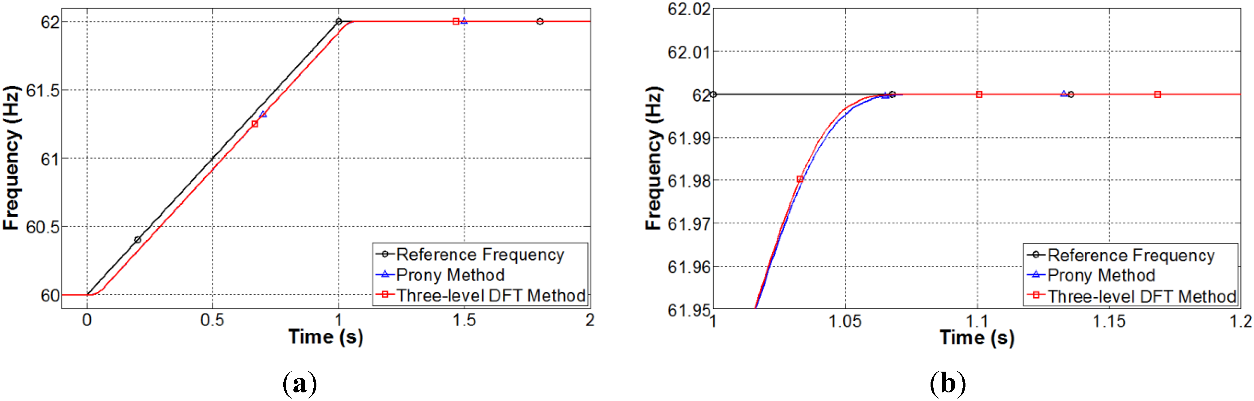
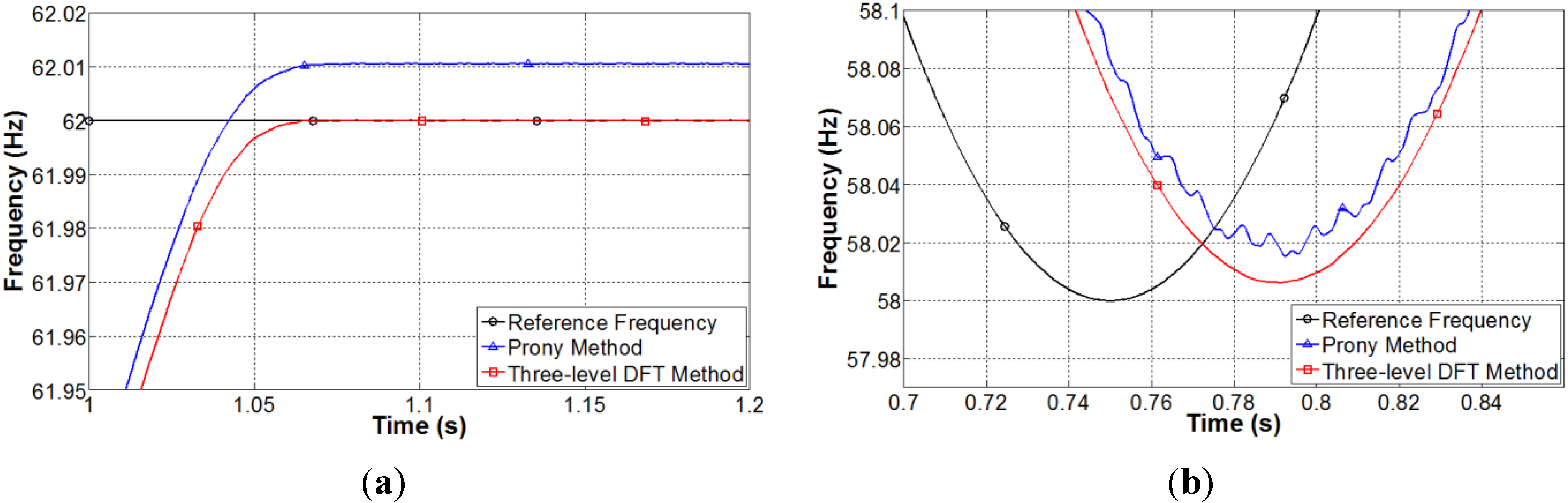
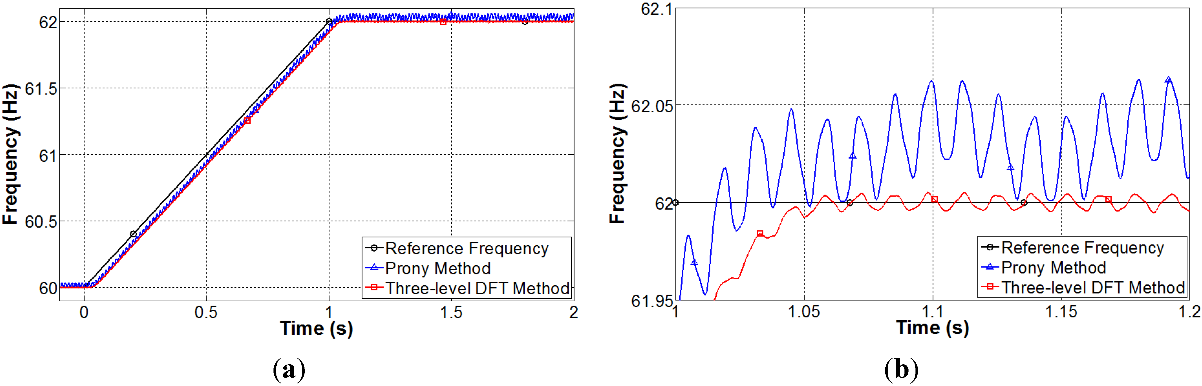
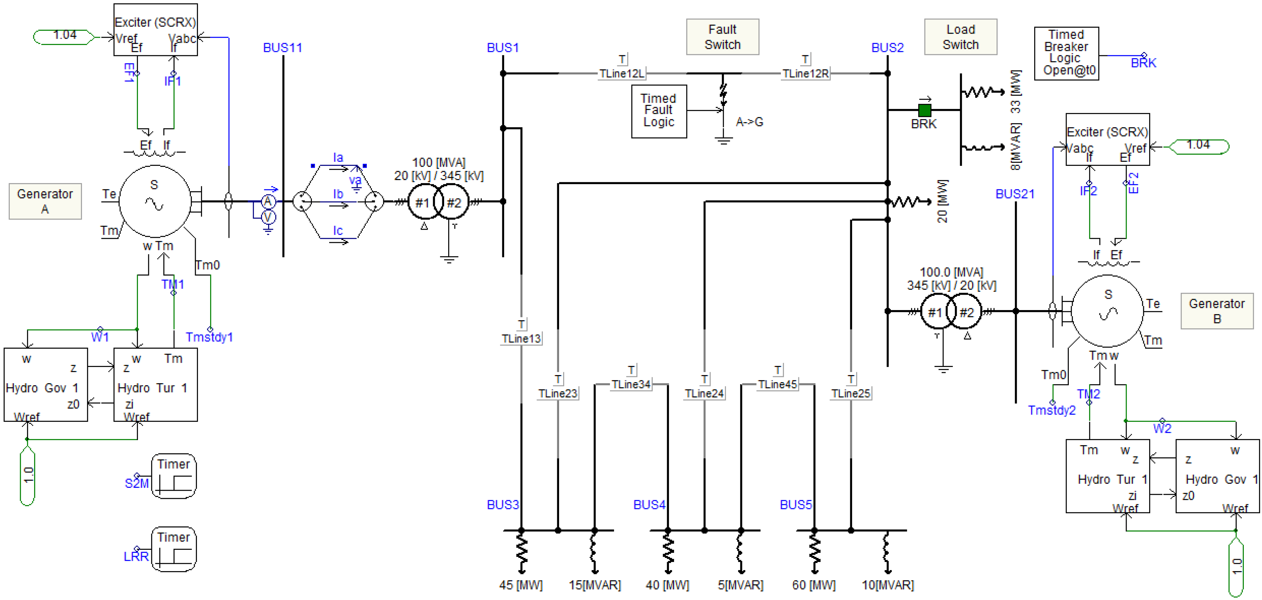
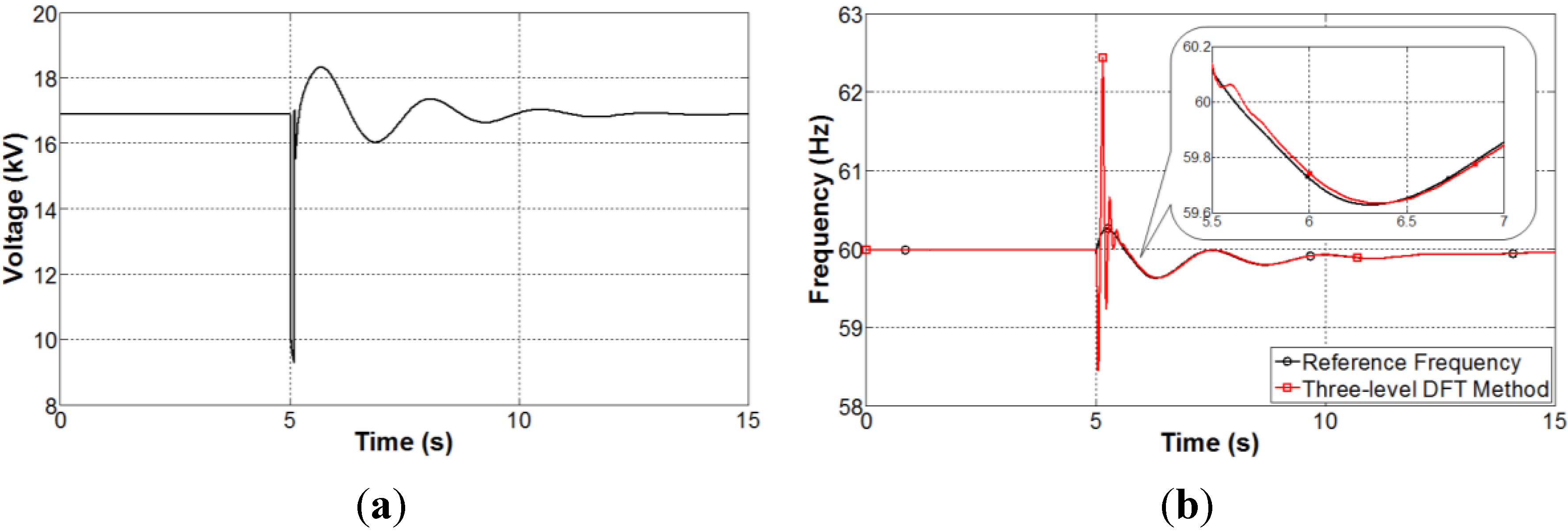
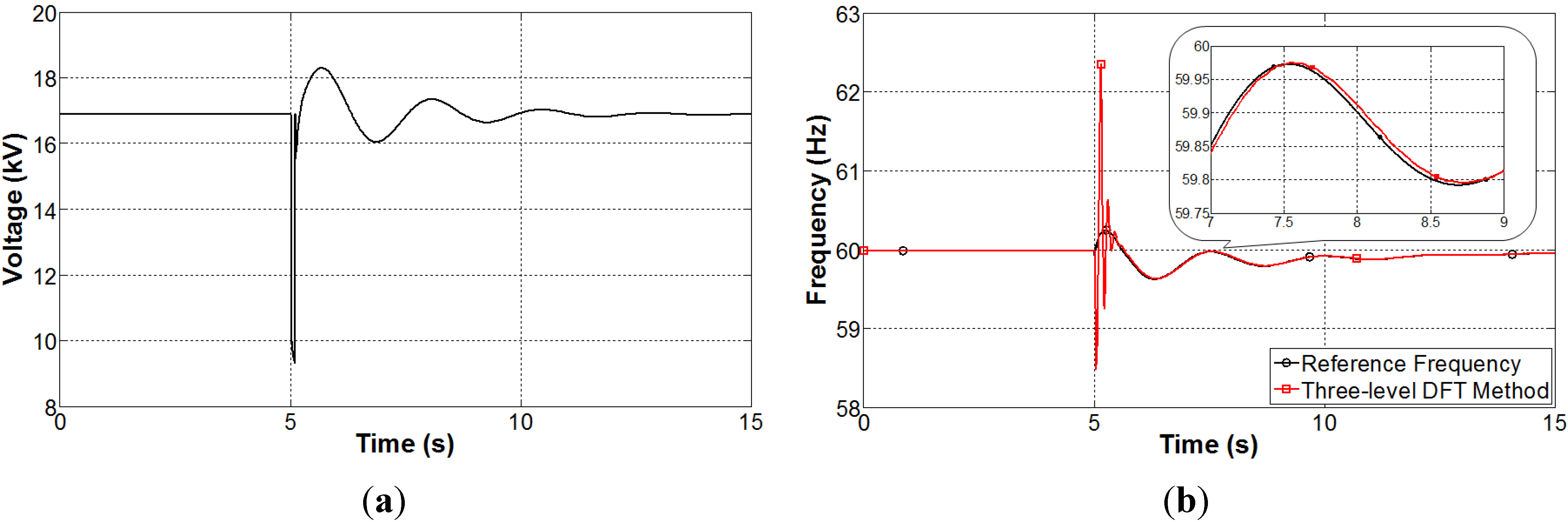
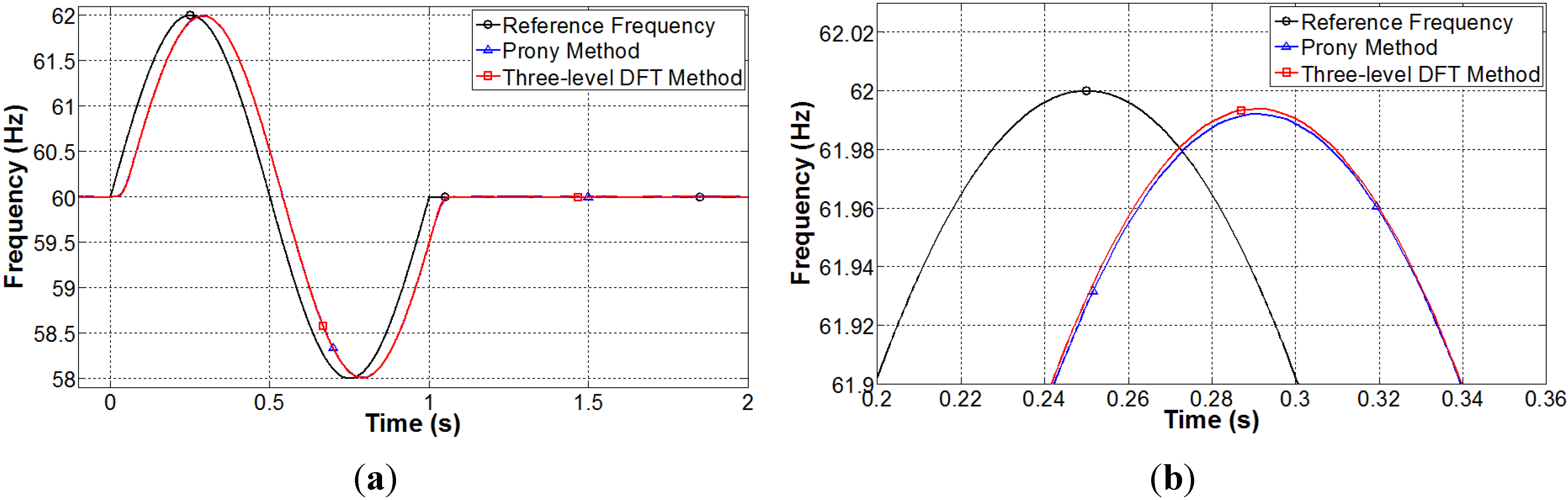
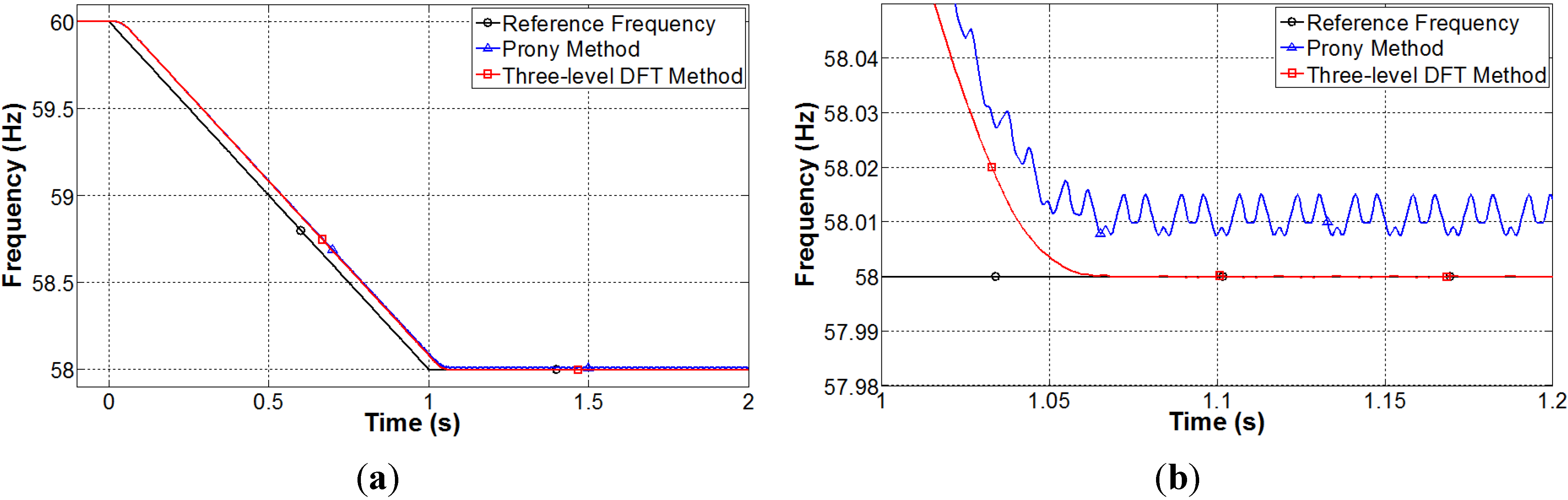
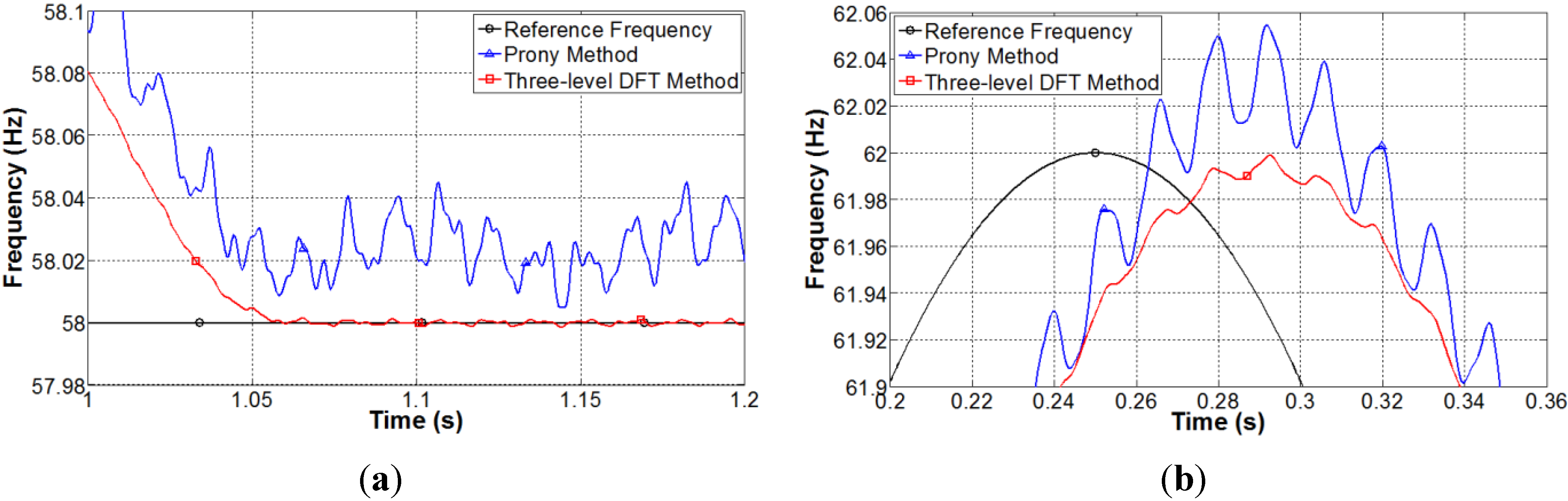
3.1. Computer Simulations

To evaluate the performance of the three-level DFT method, the results were compared with those obtained using the Prony method [1], which is one of the most commonly used orthogonal approaches to estimate the power system frequency. The Prony method estimates the power system frequency by applying Prony analysis to a sine-filtered signal:

$$f=\frac{N_0{f}_0}{2\text{π}}{\text{cos}}^{-1}(\frac{{\displaystyle \sum _{m=2}^{M-1}{\{x_S(m-1)+x_S(m+1)\}}^2}}{2{\displaystyle \sum _{m=2}^{M-1}{x}_S(m)\cdot \{x_S(m-1)+x_S(m+1)\}}})$$

(25)

where M is the total number of sine-filtered samples used to calculate the best estimate of the power system frequency. Considering that the three-level DFT method requires three cycles, here we also used the Prony method with the same amount of samples for the sake of comparison. Since one-cycle samples are required for the sine filter in the Prony method, $M$ was set to the number of samples corresponding to two cycles. In the simulations, a moving average filter with a length of two cycles was applied at the last step to obtain a stable response. Therefore, both the Prony and three-level DFT methods used five cycles as a data window.

The simulation results described in this section were processed using Matlab, and the sampling frequency was set to 1920 Hz (32 samples per cycle in a 60-Hz system). To evaluate the performance of the three-level DFT method, three types of frequency variation were considered: a ramp-up frequency variation:

$$f_1(n)=f_0+\frac{2\cdot n}{f_0{N}_0}\{u(n)-u(n-f_0{N}_0)\}+2\cdot u(n-f_0{N}_0)$$

(26)

where $u(n)$ is the unit-step function, a ramp-down frequency variation:

$$f_2(n)=f_0-\frac{2\cdot n}{f_0{N}_0}\{u(n)-u(n-f_0{N}_0)\}-2\cdot u(n-f_0{N}_0)$$

(27)

and a sinusoidal frequency variation:

$$f_3(n)=f_0+2\cdot \text{sin}(2\text{π}\frac{n}{f_0{N}_0})\{u(n)-u(n-f_0{N}_0)\}$$

(28)

A clean signal described by Equation (29) was provided as an input to both the Prony and three-level DFT methods:

$$x_1(n)=1.00\times \text{sin}(2\text{π}\frac{f_k(n)}{f_0}\frac{n}{N_0})$$

(29)

where $f_k(n)$ denotes the type of frequency variation. As shown in Figure 2, the two methods have an almost identical time response to the ramp-up frequency variation, except that the three-level DFT converges to the final reference frequency slightly faster than the Prony method (by 2.75 ms).

Figure 2. Estimation of a ramp-up frequency variation. (a) Estimated frequency; (b) Close-up of the convergence.

Figure 2. Estimation of a ramp-up frequency variation. (a) Estimated frequency; (b) Close-up of the convergence.

With the sinusoidal frequency variation, the two methods also had an almost identical time response, as shown in Figure 3. The Prony and three-level DFT methods estimated the peak frequency to be smaller than the reference frequency by 0.008 and 0.006 Hz, respectively, due to the smoothing effect of the moving average filter.

Figure 3. Estimation of a sinusoidal frequency variation. (a) Estimated frequency; (b) Close-up of the convergence.

Figure 3. Estimation of a sinusoidal frequency variation. (a) Estimated frequency; (b) Close-up of the convergence.

To investigate the influence of harmonics, the following signal with a total harmonic distortion of 30% was considered:

$$x_2(n)=1.0\times \text{sin}(2\text{π}n\frac{f_k(n)}{f_s})+0.2\times \text{sin}(2\text{π}n\frac{2f_k(n)}{f_s})+0.2\times \text{sin}(2\text{π}n\frac{3f_k(n)}{f_s})+0.1\times \text{sin}(2\text{π}n\frac{5f_k(n)}{f_s})$$

(30)

Figure 4 and Figure 5 demonstrate the ability of the three-level DFT method clearly. When the reference frequency was close to the nominal frequency in the presence of harmonics, the simulation results show a good response of both methods; however, when the reference frequency deviated from the nominal frequency, the Prony method resulted in considerable errors. In contrast, the time responses of the three-level DFT method were almost identical to those for the clean signal. This is because triple use of DFTs allows accurate frequency estimation that is insensitive to harmonics.

Figure 4. Estimation of a ramp-down frequency variation in the presence of harmonics. (a) Estimated frequency; (b) Close-up of the convergence.

Figure 4. Estimation of a ramp-down frequency variation in the presence of harmonics. (a) Estimated frequency; (b) Close-up of the convergence.

Figure 5. Estimation of ramp-up and sinusoidal frequency variations in the presence of harmonics. (a) Ramp-up frequency variation; (b) Sinusoidal frequency variation.

Figure 5. Estimation of ramp-up and sinusoidal frequency variations in the presence of harmonics. (a) Ramp-up frequency variation; (b) Sinusoidal frequency variation.

The effect of inter-harmonics in the signals was evaluated using the following signal:

$$x_3(n)=1.0\times \text{sin}(2\text{π}n\frac{f_k(n)}{f_0{N}_0})+0.2\times \text{sin}(2\text{π}n\frac{2f_k(n)}{f_0{N}_0})+0.2\times \text{sin}(2\text{π}n\frac{3f_k(n)}{f_0{N}_0})+0.1\times \text{sin}(2\text{π}n\frac{5f_k(n)}{f_0{N}_0})+0.1\times \text{sin}(2\text{π}n\frac{2.2f_k(n)}{f_0{N}_0})+0.1\times \text{sin}(2\text{π}n\frac{3.5f_k(n)}{f_0{N}_0})$$

(31)

Figure 6 and Figure 7 demonstrate the ability of the three-level DFT method in the presence of inter-harmonics in addition to harmonics. A comparison of Figure 5a and Figure 6 shows that inter-harmonics have an adverse effect on both methods in the case of the ramp-up frequency variation. Although the effect of inter-harmonics resulted in some errors, the three-level DFT method exhibit improved frequency estimation compared with the Prony method. This is because triple use of DFTs allows accurate frequency estimation that is insensitive to harmonics and inter-harmonics. Similar results can be confirmed by comparing Figure 4 with Figure 7a, which shows the response of the two methods to the ramp-down frequency variation.

Figure 6. Estimation of a ramp-up frequency variation in the presence of harmonics and inter-harmonics. (a) Estimated frequency; (b) Close-up of the convergence.

Figure 6. Estimation of a ramp-up frequency variation in the presence of harmonics and inter-harmonics. (a) Estimated frequency; (b) Close-up of the convergence.

Figure 7. Estimation of ramp-down and sinusoidal frequency variations in the presence of harmonics and inter-harmonics. (a) Ramp-down frequency variation; (b) Sinusoidal frequency variation.

Figure 7. Estimation of ramp-down and sinusoidal frequency variations in the presence of harmonics and inter-harmonics. (a) Ramp-down frequency variation; (b) Sinusoidal frequency variation.

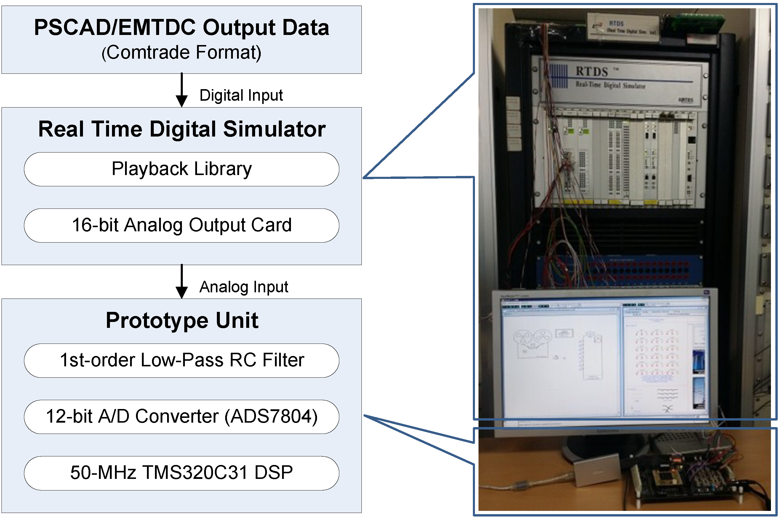
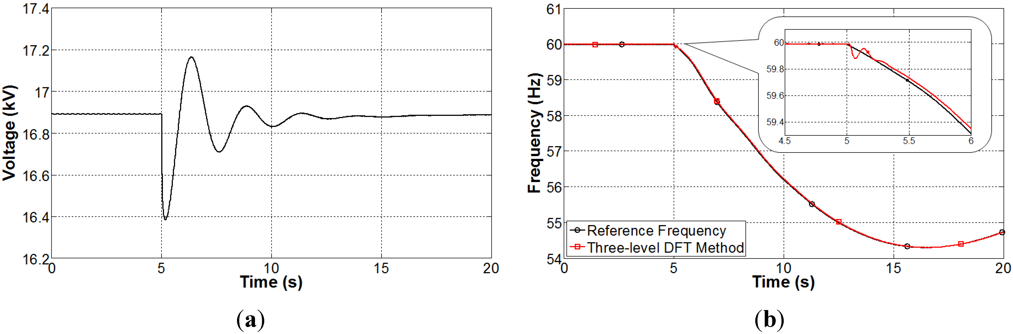
3.2. Hardware Implementation

The three-level DFT method was implemented on a 50-MHz TMS320C31 DSP-based hardware prototype. Its performance in the hardware implementation was evaluated through the testing procedure shown in Figure 8.

Figure 8. Hardware implementation.

Figure 8. Hardware implementation.

PSCAD/EMTDC was used to simulate the voltage and rotor-speed waveforms of the modified IEEE 5-bus system shown in Figure 9. The simulated voltage waveform was imported to the real-time digital simulator (RTDS) and Playback library in the RTDS generated a 16-bit analog voltage waveform in the range ±10 V. This voltage waveform was passed through a first-order low-pass RC filter to a 12-bit analog-to-digital (A/D) converter on the hardware prototype. The −3-dB cutoff frequency of the low-pass RC filter was 132 Hz, and the sampling rate of the A/D converter was 1920 Hz. The three-level DFT method completed real-time estimation of the power system frequency within each timer-interrupt interval of the DSP (520.83 µs), which corresponds to the sampling rate of the A/D converter.

In the modified IEEE 5-bus system, two 200-MVA generators supplied electric power to the load, which was initially set to 170 MVA (0.97 lag). Two types of dynamic conditions were considered: a load increase and single phase-to-ground faults.

The load switch shown in Figure 9 was closed at time t = 5.00 s, thus loading the generators with an additional 34 MVA. This caused the terminal voltage of generator A to decrease instantaneously from 16.89 kV to 16.39 kV, as shown in Figure 10a. The estimated frequency using the three-level DFT method implemented on the DSP-based hardware prototype is shown in Figure 10b together with the reference frequency, which corresponds to the rotor speed obtained from the PSCAD/EMTDC simulation. The instantaneous variation in the terminal voltage was responsible for a −0.11-Hz spike at 5.05 s in the estimated frequency. There is, of course, no corresponding instantaneous variation in the rotor speed, and so the power system frequency did not vary in the same manner. Disregarding this artifact, Figure 10b clearly shows that the estimated frequency of the three-level DFT method closely followed the reference frequency with an estimation delay of approximately 0.04 s.

Figure 9. Modified IEEE 5-bus system.

Figure 9. Modified IEEE 5-bus system.

Figure 10. Estimation of the power system frequency when the total load increased by 20%. (a) Terminal voltage of generator A; (b) Estimated frequency.

Figure 10. Estimation of the power system frequency when the total load increased by 20%. (a) Terminal voltage of generator A; (b) Estimated frequency.

The fault switch shown in Figure 9 was closed at t = 5.00 s and then opened at t = 5.10 s, creating an “a” phase-to-ground (a-g) 90° fault with a duration of 0.10 s. As shown in Figure 11a, the a-g 90° fault caused the amplitude of the generator terminal voltage to decrease instantaneously from 16.89 kV to 9.31 kV. This instantaneous decrease in the terminal voltage caused a −1.54-Hz spike at 5.06 s in the estimated frequency of the three-level DFT method. After removing the fault at 5.10 s, the generator terminal voltage increased to 18.33 kV and then settled to the initial value. Due to the instantaneous increase in the terminal voltage, the estimated frequency had a 2.45-Hz spike at 5.16 s.

Figure 11. Estimation of the power system frequency when a single line-to-ground 90° fault occurred. (a) Terminal voltage of generator A; (b) Estimated frequency.

Figure 11. Estimation of the power system frequency when a single line-to-ground 90° fault occurred. (a) Terminal voltage of generator A; (b) Estimated frequency.

Similar to the a-g 90° fault, the fault switch was closed at t = 5.00 s and then opened at t = 5.10 s, creating an a-g 0° fault. As shown in Figure 12b, the instantaneous decrease in the terminal voltage caused a −1.51-Hz spike at 5.05 s in the estimated frequency of the three-level DFT method. After removing the fault at 5.10 s, the estimated frequency had a 2.37-Hz spike at 5.15 s.

With the exception of the spikes during the a-g faults, the estimated frequency using the three-level DFT method followed the reference frequency closely. These results show that the hardware prototype can accurately estimate the power system frequency in real time.

Figure 12. Estimation of the power system frequency when a single line-to-ground 0° fault occurred. (a) Terminal voltage of generator A; (b) Estimated frequency.

Figure 12. Estimation of the power system frequency when a single line-to-ground 0° fault occurred. (a) Terminal voltage of generator A; (b) Estimated frequency.

4. Conclusions

We have proposed a three-level DFT method for real-time estimation of power system frequency. The method is based on the fact that the amplitude gains of cosine and sine filters differ when the power system frequency deviates from the nominal frequency. Since the amplitude ratio of the cosine- and sine-filtered signals should be known prior to estimating the power system frequency, a second-level DFT was applied to these cosine- and sine-filtered signals. Although the amplitude ratio can be determined using the output signals of the second-level DFT, the errors in the amplitude ratio may be large when the output signals of the second-level DFT are near to a zero crossing. To overcome this problem, a third-level DFT was applied to the output signals of the second-level DFT. After the amplitude ratio was accurately determined using the output signals of the third-level DFT, the power system frequency was estimated. This triple use of DFTs allows accurate frequency estimation that is insensitive to harmonics and inter-harmonics. Although the three-level DFT method may lead to an additional two-cycle delay compared with other DFT-based orthogonal approaches, it is fast enough to be used in rapid-response applications where the transient response should be no longer than five cycles.

The performance of the three-level DFT method was evaluated using computer-simulated signals with harmonics and inter-harmonics. The simulation results confirmed that the method was able to estimate the power system frequency accurately, even in the presence of harmonics and inter-harmonics. The method was then implemented on a TMS320C31 DSP-based hardware prototype. The RTDS was used to evaluate its performance under dynamic conditions, including a load increase and single phase-to-ground faults on the modified IEEE 5-bus system. The results of this implementation showed that the hardware prototype was able to accurately estimate the power system frequency in real time.

References

1. Lobos, T.; Rezmer, J. Real-time determination of power system frequency. IEEE Trans. Instrum. Meas. 1997, 46, 877–881. [Google Scholar] [CrossRef]
2. Rahmann, C.; Castillo, A. Fast frequency response capability of photovoltaic power plants: The necessity of new grid requirements and definitions. Energies 2014, 7, 6306–6322. [Google Scholar] [CrossRef]
3. Margaris, I.D.; Hansen, A.D.; Sørensen, P.; Hatziargyriou, N.D. Illustration of modern wind turbine ancillary services. Energies 2010, 3, 1290–1302. [Google Scholar] [CrossRef]
4. Thomas, D.W.P.; Woolfson, M.S. Evaluation of frequency tracking methods. IEEE Trans. Power Deliv. 2001, 16, 367–371. [Google Scholar] [CrossRef]
5. Denis, P.; Counan, C.; Hossenlopp, L.; Holweck, C. Measurement of voltage phase for the French future defence plan against losses of synchronism. IEEE Trans. Power Deliv. 1992, 7, 62–69. [Google Scholar] [CrossRef]
6. Begovic, M.M.; Djuric, P.M.; Dunlap, S.; Phadke, A.G. Frequency tracking in power network in the presence of harmonics. IEEE Trans. Power Deliv. 1993, 8, 480–486. [Google Scholar] [CrossRef]
7. Akke, M. Frequency estimation by demodulation of two complex signals. IEEE Trans. Power Deliv. 1997, 12, 157–163. [Google Scholar] [CrossRef]
8. Moore, P.J.; Carranza, R.D.; Johns, A.T. A new numeric technique for high-speed evaluation of power system frequency. IEE Proc.-Gener. Transm. Distrib. 1994, 141, 529–536. [Google Scholar] [CrossRef]
9. Sidhu, T.S. Accurate measurement of power system frequency using a digital signal processing technique. IEEE Trans. Instrum. Meas. 1999, 48, 75–81. [Google Scholar] [CrossRef]
10. Nam, S.R.; Lee, D.G.; Kang, S.H.; Ahn, S.J.; Choi, J.H. Power system frequency estimation in power systems using complex prony analysis. Int. J. Electr. Eng. Technol. 2011, 6, 154–160. [Google Scholar] [CrossRef]
11. Phadke, A.G.; Thorp, J.S.; Adamiak, M.G. A new measurement technique for tracking voltage phasors, local system frequency and rate of change of frequency. IEEE Trans. Power Appl. Syst. 1983, PAS-102, 1025–1038. [Google Scholar] [CrossRef]
12. Yang, J.Z.; Liu, C.W. A precise calculation of power system frequency. IEEE Trans. Power Deliv. 2001, 16, 361–366. [Google Scholar] [CrossRef]
13. Jinfeng, R.; Kezunovic, M. A hybrid method for power system frequency estimation. IEEE Trans. Power Deliv. 2012, 27, 1252–1259. [Google Scholar] [CrossRef]
14. Djuric, M.B.; Djurisic, Z.R. Frequency measurement of distorted signals using Fourier and zero crossing techniques. Electr. Power Syst. Res. 2008, 78, 1407–1415. [Google Scholar] [CrossRef]
15. Eckhardt, V.; Hippe, P.; Hosemann, G. Dynamic measuring of frequency and frequency oscillations in multiphase power systems. IEEE Trans. Power Deliv. 1989, 4, 95–102. [Google Scholar] [CrossRef]
16. Kaura, V.; Blasko, V. Operation of a phase locked loop system under distorted utility conditions. IEEE Trans. Ind. Appl. 1997, 33, 58–63. [Google Scholar] [CrossRef]
17. Karimi, H.; Karimi-Ghartemani, M.; Iravani, M.R. Estimation of frequency and its rate of change for application in power systems. IEEE Trans. Power Deliv. 2004, 19, 472–480. [Google Scholar] [CrossRef]
18. Girgis, A.A.; Hwang, T.L. Optimal estimation of voltage and frequency deviation using linear and non-linear Kalman filtering: Theory and limitations. IEEE Trans. Power Appar. Syst. 1984, 103, 2943–2949. [Google Scholar] [CrossRef]
19. Dash, P.K.; Pradhan, A.K.; Panda, G. Frequency estimation of distorted power system signals using extended complex Kalman filter. IEEE Trans. Power Deliv. 1999, 14, 761–766. [Google Scholar] [CrossRef]
20. Routray, A.; Pradhan, A.K.; Rao, K.P. A novel Kalman filter for frequency estimation of distorted signals in power system. IEEE Trans. Instrum. Meas. 2002, 51, 469–479. [Google Scholar] [CrossRef]
21. Zadeh, R.A.; Ghosh, A.; Ledwich, G. Combination of Kalman filter and least-error square techniques in power system. IEEE Trans. Power Deliv. 2010, 25, 2868–2880. [Google Scholar] [CrossRef] [Green Version]
22. Kamwa, I.; Grondin, R. Fast adaptive schemes for tracking voltage phasor and local frequency in power transmission and distribution systems. IEEE Trans. Power Deliv. 1992, 7, 789–795. [Google Scholar] [CrossRef]
23. Zivanovic, R. An adaptive differentiation filter for tracking instantaneous frequency in power system. IEEE Trans. Power Deliv. 2007, 22, 765–771. [Google Scholar] [CrossRef]
24. Mojiri, M.; Karimi-Ghartemani, M.; Bakhshai, A. Estimation of power system frequency using an adaptive notch filter. IEEE Trans. Instrum. Meas. 2007, 56, 2470–2477. [Google Scholar] [CrossRef]
25. Rawat, T.K.; Parthasarathy, H. A continuous-time least mean-phase adaptive filter for power system frequency estimation. Int. J. Electr. Power Energy Syst. 2009, 31, 111–115. [Google Scholar] [CrossRef]
26. Xia, Y.; Mandic, D.P. A widely linear least mean phase algorithm for adaptive frequency estimation of unbalanced power systems. Int. J. Electr. Power Energy Syst. 2014, 54, 367–375. [Google Scholar] [CrossRef]
27. Sachdev, M.S.; Giray, M.M. A least square technique for determining power system frequency. IEEE Trans. Power Appl. Syst. 1985, 437, 437–443. [Google Scholar] [CrossRef]
28. Giray, M.M.; Sachdev, M.S. Off-nominal frequency measurements in electric power systems. IEEE Trans. Power Deliv. 1989, 4, 1573–1578. [Google Scholar] [CrossRef]
29. Pradhan, A.K.; Routray, A.; Basak, A. Power system frequency estimation using least mean square technique. IEEE Trans. Power Deliv. 2005, 20, 1812–1816. [Google Scholar] [CrossRef]
30. Chundamani, R.; Vasudevan, K.; Ramalingam, C.S. Real-time estimation of power system frequency using nonlinear least squares. IEEE Trans. Power Deliv. 2009, 24, 1021–1028. [Google Scholar] [CrossRef]
31. Alkandari, A.M.; Soliman, S.A. Measurement of a power system nominal voltage, frequency and voltage flicker parameters. Int. J. Electr. Power Energy Syst. 2009, 31, 295–301. [Google Scholar] [CrossRef]
32. Abdollahi, A.; Matinfar, F. Frequency estimation: A least-squares new approach. IEEE Trans. Power Deliv. 2011, 26, 790–798. [Google Scholar] [CrossRef]
33. Dash, P.K.; Swain, D.P.; Routray, A.; Liew, A.C. An adaptive neural network approach for the estimation of power system frequency. Electr. Power Syst. Res. 1997, 41, 203–210. [Google Scholar] [CrossRef]
34. Lai, L.L.; Chan, W.L.; Tse, C.T.; So, A.T.P. Real-time frequency and harmonic evaluation using artificial neural networks. IEEE Trans. Power Deliv. 1999, 14, 52–59. [Google Scholar] [CrossRef]
35. Terzija, V.V.; Djuric, M.B.; Kovacevic, B.D. Voltage phasor and local system frequency estimation using Newton type algorithm. IEEE Trans. Power Deliv. 1994, 9, 1368–1374. [Google Scholar] [CrossRef]
36. Zheng, J.; Lui, K.W.K.; Ma, W.K.; So, H.C. Two simplified recursive gauss–newton algorithms for direct amplitude and phase tracking of a real sinusoid. IEEE Signal Process. Lett. 2007, 14, 972–975. [Google Scholar] [CrossRef]
37. Xue, S.Y.; Yang, S.X. Power system frequency estimation using Supervised Gauss-Newton algorithm. Measurement 2009, 42, 28–37. [Google Scholar] [CrossRef]
38. Dash, P.K.; Krishnanand, K.R.; Patnaik, R.K. Dynamic phasor and frequency estimation of time-varing power system signals. Int. J. Electr. Power Energy Syst. 2013, 44, 971–980. [Google Scholar] [CrossRef]
39. Lin, T.; Tsuji, M.; Yamada, E. A wavelet approach to real time estimation of power system frequency. In Proceedings of the 40th SICE Annual Conference, Nagoya, Japan, 25–27 July 2001; pp. 58–65.
40. Ren, J.; Kezunovic, M. Use of recursive wavelet transform for estimating power system frequency and phasors. In Proceedings of the Transmission and Distribution Conference and Exposition, New Orleans, LA, USA, 19–22 April 2010; pp. 1–6.
41. Jinfeng, R.; Kezunovic, M. Real-Time power system frequency and phasors estimation using recursive wavelet transform. IEEE Trans. Power Deliv. 2011, 26, 1392–1402. [Google Scholar] [CrossRef]