A Dynamic Economic Dispatch Model Incorporating Wind Power Based on Chance Constrained Programming

Abstract

In order to maintain the stability and security of the power system, the uncertainty and intermittency of wind power must be taken into account in economic dispatch (ED) problems. In this paper, a dynamic economic dispatch (DED) model based on chance constrained programming is presented and an improved particle swarm optimization (PSO) approach is proposed to solve the problem. Wind power is regarded as a random variable and is included in the chance constraint. New formulation of up and down spinning reserve constraints are presented under expectation meaning. The improved PSO algorithm combines a feasible region adjustment strategy with a hill climbing search operation based on the basic PSO. Simulations are performed under three distinct test systems with different generators. Results show that both the proposed DED model and the improved PSO approach are effective.

1. Introduction

Dynamic economic dispatch (DED), which determines the optimal generation scheme to meet the predicted load demand over a time horizon satisfying the constraint such as ramp-rate limits of generators between time intervals, is crucial for power system operation [1,2,3]. Prior to the widespread use of alternate sources (solar, wind) of energy, the DED problem involved only conventional generators. In recent years, wind power has experienced an explosive growth, and has shown great potential in fuel savings and environmental protection. However, its uncertainty and intermittency also makes it challenging to find a proper dispatch scheme for a wind penetrated power system.

The key issue associated with the incorporation of wind power is how to deal with its fluctuation and intermittence considering the required reliability and security of power systems [2]. Up to now, different authors have proposed models to solve economic dispatch (or unit commitment) problems for wind-penetrated power systems [4,5,6,7,8,9,10,11,12,13,14,15,16]. Chen [4] proposed a method to incorporate wind generators into the generation scheduling problem. Special reserve constraints are established to operate the power system within the required stability margin, which is also adopted by Zhou et al. [5] and Jiang et al. in [6]. These models are deterministic and cannot accurately describe the effect of wind fluctuations on system operation.

To effectively and safely use wind power, researchers usually forecast the wind speed or wind generation over a time horizon in advance, and then obtain the statistic distribution of wind speed or wind generation. Based on the distribution function and estimated loads, researchers can determine the dispatch scheme. Hetzer et al. presented an ED model incorporating wind power with the stochastic wind speed characterization based on the Weibull probability density function [7]. Penalty costs for overestimation and underestimation of available wind energy are also considered. In [8], a modified ED optimization model with wind power penetration is presented, and risk-based up and down spinning reserve constraints are presented considering the uncertainties of available wind power, load forecast error and also generator outage rates. It has been discussed in [9,10,11] that forecasted wind generation usually follows a beta distribution function, and following this, the authors of [12] and [13] proposed ED models incorporating the impact of wind variability. Miranda and Hang developed in [14] an ED model including wind generators using concepts from the fuzzy set theory, and they added a penalty cost factor for not using the available wind power capacity. It is noted clearly in references [7,8,12,13,14] that the constraints of ramp rates are not taken into account. In [15] and [16], a scenario-based approach is utilized to model the uncertainty of wind power and stochastic models are proposed to solve the optimal scheduling of the generators in wind penetrated power system. This scenario approach requires a large number of scenarios to ensure the quality of solution, and usually suffers huge computation cost.

Chance constrained programming (CCP) is a kind of stochastic optimization approach [17]. It is suitable for solving optimization problems with random variables either included in constraints or in the objective function. CCP has been studied to solve the transmission planning problem in [17,18] and the stochastic unit commitment problem with uncertain wind power output in [19]. In [17] and [18], the same formulation of chance constraint is applied to transmission planning, and it is in the form that the not-overload probability for transmission line is required to be more than a specified confidence level. In [19], the chance constraint is applied to describe policies to ensure the utilization of wind power, and a two stage stochastic optimization is presented to solve the unit commitment problem. In this paper, the chance constraint is used to describe that the probability that actual wind generation is greater than or equal to the scheduled wind power is more than a given confidence level.

In a manner somewhat similar to the wind model in [12] and [13], this paper uses a beta distribution to characterize the actual wind generation for each individual period. Up spinning reserve (USR) and down spinning reserve (DSR) are required to deal with the forecasting errors in load and the sudden fluctuations in wind generation [15]. In general, the reserve requirement with respect to forecast errors in load is defined to be a fixed percentage [5] (e.g., 5%) of the load demand. As to the reserve requirements caused by variation of wind generation, up reserve requirement (URR) induced by the sudden fall in wind generation and down reserve requirement (DRR) induced by the sudden raise in wind generation are both taken into account in our work. The conditional expectation when actual wind generation is smaller than the scheduled wind is calculated, and URR is defined as the difference between the scheduled wind power and the conditional expectation of wind power. Similarly, DRR is defined as the difference between the conditional expectation when actual wind generation is greater than or equal to the scheduled wind power and the scheduled wind power.

This paper proposes a stochastic DED model based on chance constraints in wind power penetrated systems. New formulations of the spinning reserve constraints are considered under the expected meaning. An improved particle swarm optimization (PSO) approach is proposed to optimize the model. In order to demonstrate the efficacy of the proposed model and the PSO approach, various comparisons are performed under two different test systems. Results show that the above-mentioned model is effective and the proposed PSO approach is able to solve such model.

The rest of this paper is organized as follows: in Section 2, the stochastic DED model is formulated. Section 3 introduces the beta distribution as the basis of the equivalent transformation of the proposed DED model, and a deterministic DED model is obtained. In Section 4, an improved PSO approach including feasible region adjustment (FRA) strategy and hill climbing search operation (HCSO) is applied to solve the deterministic model. Section 5 presents a discussion of the numerical results. Finally, conclusions are drawn in Section 6.

2. DED Problem Formulation

In this section, the objective function of DED problem is described and the DED model based on CCP is formulated.

2.1. Objective Function

In wind penetrated power systems, wind production is usually regarded as zero cost, the DED model with the valve point effect usually takes the following form [20,21,22,23,24]:

$$\text{min} f_{\text{cos}t}={\displaystyle \sum _{t=1}^T{\displaystyle \sum _{i=1}^I[C_i(p_{i,t})+E_i(p_{i,t})]}}$$

(1)

where:

• $f_{\text{cos}t}$ is the total generation cost over the whole time horizon;
• $T$ is the number of periods;
• $I$ is the number of thermal units;
• $p_{i,t}$ is the power output (MW) of the $i$th unit corresponding to time period $t$;
• $C_i(p_{i,t})$ is the generation cost of the $i$th unit corresponding to time period $t$;
• $E_i(p_{i,t})$ is the valve point loading effect of the $i$th unit corresponding to time period $t$;

For the thermal units, the generation cost can be approximated by a quadratic function of the power output, which is practical for most of the cases, and is given by:

$$C_i(p_{i,t})=a_i{p}_{i,t}^2+b_i{p}_{i,t}+c_i$$

(2)

where $a_i$, $b_i$ and $c_i$ are cost coefficients for the $i$th unit. $E_i(p_{i,t})$ is expressed as follows:

$$E_i(p_{i,t})=\left|e_i\text{sin}[f_i(p_{i\text{min}}-p_{i,t})]\right|$$

(3)

where $e_i$ and $f_i$ are coefficients related to valve point effect of the ith unit. $p_{i\text{min}}$ is the minimum generation limit of unit i.

2.2. System and Unit Constraints

This DED problem is subjected to a variety of system and unit constraints, which include power balance constraints, generation limits of units, ramp rate limits and spinning reserve constraints. These constraints are discussed below.

2.2.1. Power Balance Constraints

Total power generation must equal the load demand p_d,t in all time period:

$${\displaystyle \sum _{i=1}^I{p}_{i,t}}+p_{w,t}=p_{d,t}$$

(4)

where p_w,t is the scheduled wind power of wind farm at time t.

2.2.2. Generation Limits of Thermal Units and Wind Farm

The output of each thermal unit and wind farm must lie in between a lower and an upper bound. These constraints are represented as follows:

$$p_{i\text{min}}\le p_{i,t}\le p_{i\text{max}}$$

(5)

$$0\le p_{w,t}\le w_{\text{max}}$$

(6)

where $p_{i\text{max}}$ is the maximum generation limit of thermal unit i, and w_max is the installed capacity of wind farm.

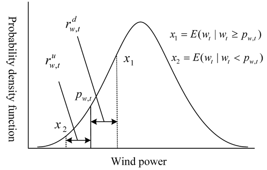
2.2.3. Chance Constraint on Wind Power

Due to the stochastic nature of wind power, the schedule for wind may not be realized on a scheduled day. So we introduce the following chance constraint:

$$P\left\{w_t\ge p_{w,t}\right\}\ge \text{ρ}$$

(7)

where w_t is a random variable representing the wind power generation at time t. ρ is the confidence level. Equation (7) defines the probability that the scheduled wind power can be realized is greater than or equal to ρ. Furthermore, Equation (7) sets a reasonable upper bound for wind power generation, and the probability that this upper bound can be realized is no less than ρ. The larger the confidence level is, the less stochastic the wind power is, and hence the more reliable the power system is. Especially, when ρ = 1, there is no wind power in system, and the DED problem is changed into a deterministic one.

2.2.4. Ramp Rate Limits of Thermal Units

The ramp rate limits restrict the operating range of all the units for adjusting the generation between two periods. The generation may adjust the dispatch level as:

$$-{\Delta }_{i,d}\times T_{60}\le p_{i,t}-p_{i,t-1}\le {\Delta }_{i,u}\times T_{60}$$

(8)

where $p_{i,t-1}$ is the output of unit i at time $t-1$, and ${\Delta }_{i,u}$ and ${\Delta }_{i,d}$ are the upper and lower ramp rate limits, respectively. T₆₀ is the operating period, i.e., 1 h.

2.2.5. Spinning Reserve Constraints

Due to the penetration of wind power and its intermittent nature, additional reserve needs to be provided to support the wind generation variation [15]. The USR supports the forecast errors in load and a sudden decrease in wind power, and the DSR contributes to the sudden raise in wind power. Both the USR and DSR are supplied by the ramping capacity of thermal units, and are formulated by Equations (9) and (10) respectively:

$${\displaystyle \sum _i^n\text{min}(p_{i,t}^{\text{max}}-p_{i,t},{\Delta }_{i,u}\times T_{10})}\ge p_{r,t}+r_{w,t}^u$$

(9)

$${\displaystyle \sum _i^n\text{min}(p_{i,t}-p_{i,t}^{\text{min}},{\Delta }_{i,d}\times T_{10})}\ge r_{w,t}^d$$

(10)

where $p_{r,t}$ is the reserve level to support forecast error in demand. T₁₀ is 10 min. $p_{i,t}^{\text{max}}$ and $p_{i,t}^{\text{min}}$ are upper and lower generation limits of unit i including ramp rate limits at time t, and $p_{i,t}^{\text{max}}=\text{min}(p_{i\text{max}},p_{i,t-1}+{\Delta }_{i,u})$, $p_{i,t}^{\text{min}}=\text{max}(p_{i\text{min}},p_{i,t-1}-{\Delta }_{i,d})$. $r_{w,t}^u$ and $r_{w,t}^d$ are the URFW and the DRRW to follow the sudden decrease and increase in wind power at time t.

Figure 1 shows the conceptual illustration of $r_{w,t}^u$ and $r_{w,t}^d$. $r_{w,t}^u$ is calculated by the difference between the scheduled wind power and conditional expectation of wind power when the actual wind generation is less than scheduled, and is shown in Equation (11):

$$r_{w,t}^u=p_{w,t}-E(w_t|w_t<p_{w,t})$$

(11)

The conditional expectation is obtained by the following equation:

$$E(w_t|w_t<p_w)=\frac{{\displaystyle {\int }_0^{p_{w,t}}{w}_t{f}_{W_t}(w_t)\text{d}{w}_t}}{{\displaystyle {\int }_0^{p_{w,t}}{f}_{W_t}(w_t)\text{d}{w}_t}}$$

(12)

where $f_{W_t}(w_t)$ is the probability density function of wind power at time t.

Similarly, $r_{w,t}^d$ is calculated using the two equations as mentioned in Equations (13) and (14):

$$r_{w,t}^d=E(w_t|w_t\ge p_{w,t})-p_{w,t}$$

(13)

$$E(w_t|w_t\ge p_w)=\frac{{\displaystyle {\int }_{p_{w,t}}^{w_{\text{max}}}{w}_t{f}_{W_t}(w_t)\text{d}{w}_t}}{{\displaystyle {\int }_{p_{w,t}}^{w_{\text{max}}}{f}_{W_t}(w_t)\text{d}{w}_t}}$$

(14)

Figure 1. Concept illustration of $r_{w,t}^u$ and $r_{w,t}^d$ .

Figure 1. Concept illustration of $r_{w,t}^u$ and $r_{w,t}^d$ .

Taking a closer look at the optimization model (1)–(14), it contains chance constraint and thus is a stochastic DED model. In the next section we will discuss the equivalent transformation of the stochastic model to a deterministic one.

3. Equivalent Transformation of the DED Model

3.1. Beta Distribution of Wind Power

In the real word, the actual wind generation is a function of wind speed that randomly changes all the time [13]. In our study, normalized wind power in each period is regarded as a random variable which follows beta distribution [9,10,11,12,13]. We denote the probability density function (PDF) by $f_{X_t}(x_t)$ as follows:

$$f_{X_t}(x_t)=\{\begin{array}{l}\frac{1}{B(\text{α},\text{β})}{x_t}^{\text{α}-1}{(1-x_t)}^{\text{β}-1},0<x_t<1\\ 0, otherwise\end{array}$$

(15)

where $x_t=w_t/w_{\text{max}}$, and $x_t\in [0,1]$. $\text{α}>0$, $\text{β}>0$, and $B(\text{α},\text{β})$ is the well-known beta function defined as:

$$B(\text{α},\text{β})={\displaystyle {\int }_0^1{u}^{\text{α}-1}{(1-u)}^{\text{β}-1}}\text{d}u$$

(16)

Parameters α and β can be determined by following equations:

$$\{\begin{array}{l}\frac{{\text{μ}}_t}{w_{\text{max}}}=\frac{\text{α}}{\text{α}+\text{β}}\\ {(\frac{{\text{σ}}_t}{w_{\text{max}}})}^2=\frac{\text{αβ}}{{(\text{α}+\text{β})}^2(\text{α}+\text{β}+1)}\end{array}$$

(17)

where ${\text{μ}}_t$ and ${\text{σ}}_t$ are the mean value and standard deviation of the predicted wind generation at time t on the scheduling day, respectively. The cumulative density function (CDF) of X can be easily obtained as shown below:

$$F_{X_t}(x)=\{\begin{array}{l}0, -\infty <x\le 0\\ \frac{1}{B(\text{α},\text{β})}{\displaystyle {\int }_0^x{u}^{\text{α}-1}{(1-u)}^{\text{β}-1}\text{d}u}, 0<x<1\\ 1, x\ge 1\end{array}$$

(18)

3.2. Equivalent Transformation

Putting the aforementioned discussion of the beta distribution, we can get the following CDF ($F_W(w_t)$) of $w_t$:

$$F_{W_t}(w_t)=\text{P}\left\{W_t\le w_t\right\}=\text{P}\left\{w_{\text{max}}{X}_t\le w_t\right\}=F_{X_t}(w_t/w_{\text{max}})$$

(19)

Then, Equations (12) and (14) are transformed into the following equations as expressed in Equations (20) and (21) respectively:

$$E(w_t|w_t<p_{w,t})=E(w_{\text{max}}{x}_t|x_t<p_{w,t}/w_{\text{max}})=w_{\text{max}}\cdot \frac{{\displaystyle {\int }_0^{p_{w,t}/w_{\text{max}}}{x}_t{f}_{X_t}(x_t)\text{d}{x}_t}}{{\displaystyle {\int }_0^{p_{w,t}/w_{\text{max}}}{f}_{X_t}(x_t)d{x}_t}}$$

(20)

$$E(w_t|w_t\ge p_{w,t})=w_{\text{max}}\cdot \frac{{\displaystyle {\int }_{p_{w,t}/w_{\text{max}}}^{w_{\text{max}}}{x}_t{f}_{X_t}(x_t)\text{d}{x}_t}}{{\displaystyle {\int }_{p_{w,t}/w_{\text{max}}}^{w_{\text{max}}}{f}_{X_t}(x_t)\text{d}{x}_t}}$$

(21)

Both Equations (20) and (21) will be solved using numerical integration methods because of the complexity. In addition, we rewrite the Equation (7) as follows:

$$P\left\{w_t\ge p_{w,t}\right\}= F_{X_t}(z)\ge \text{ρ}$$

(22)

where $p_{w,t}/w_{\text{max}}=z$, form $F_{X_t}(z)=\text{ρ}$, we learn that z is the upper quantile of $F_{X_t}(x_t)$, then we get $p_{w,t}\le w_{\text{max}}\cdot F_{X_t}^{-1}(1-\text{ρ})$, and thus obtain the following constraint of scheduled wind power:

$$0\le p_{w,t}\le w_{\text{max}}\cdot F_{X_t}^{-1}(1-\text{ρ})$$

(23)

Given all that, the equivalent transformation of the stochastic DED model is mathematically represented as:

$$\{\begin{array}{l}\text{min}{\displaystyle \sum _{t=1}^T{\displaystyle \sum _{i=1}^I\left\{a_i{p}_{i,t}^2+b_i{p}_{i,t}+c_i+\left|e_i\text{sin}[f_i(p_{i\text{min}}-p_{i,t})]\right|\right\}}}\hfill \\ s.t.\begin{array}{l}{\displaystyle \sum _{i=1}^I{p}_{i,t}}+p_{w,t}=p_{d,t}\hfill \\ p_{i\text{min}}\le p_{i,t}\le p_{i\text{max}}\hfill \\ 0\le p_{w,t}\le w_{\text{max}}\cdot F_{X_t}^{-1}(1-\text{ρ})\hfill \\ -{\Delta }_{i,d}\times T_{60}\le p_{i,t}-p_{i,t-1}\le {\Delta }_{i,u}\times T_{60}\hfill \\ {\displaystyle \sum _i^I\text{min}(p_{i,t}^{\text{max}}-p_{i,t},{\Delta }_{i,u}\times T_{10})}\ge p_{r,t}+p_{w,t}-w_{\text{max}}\cdot \frac{{\displaystyle {\int }_0^{p_{w,t}/w_{\text{max}}}{x}_t{f}_{X_t}(x_t)\text{d}{x}_t}}{{\displaystyle {\int }_0^{p_{w,t}/w_{\text{max}}}{f}_{X_t}(x_t)\text{d}{x}_t}}\hfill \\ {\displaystyle \sum _i^I\text{min}(p_{i,t}-p_{i,t}^{\text{min}},{\Delta }_{i,d}\times T_{10})}\ge w_{\text{max}}\cdot \frac{{\displaystyle {\int }_{p_{w,t}/w_{\text{max}}}^1{x}_t{f}_{X_t}(x_t)\text{d}{x}_t}}{{\displaystyle {\int }_{p_{w,t}/w_{\text{max}}}^1{f}_{X_t}(x_t)\text{d}{x}_t}}-p_{w,t}\hfill \end{array}\hfill \end{array}$$

(24)

4. Improved PSO Approach

The problem in Equation (24) is a high-dimension and non-convex optimization problem, so it is very difficult to find analytical solutions. In recent decades, many salient approaches have been developed to solve such problems, such as genetic algorithm [20,21], differential evolution [22], evolutionary programming [25,26], and PSO [6,27,28,29,30,31,32]. PSO, first introduced by Kennedy and Eberhart, is a population-based optimization technique, and conducts its search using a population of particles [27,28]. Each particle is a candidate solution to the problem and is moved toward the optimal point by adding a velocity with its position. The position and the velocity of the jth particle in the D dimensional search space can be expressed as $Y_j={[y_{j1},y_{j2},\cdots ,y_{jD}]}^{\text{T}}$ and $V_j={[v_{j1},v_{j2},\cdots ,v_{jD}]}^{\text{T}}$, respectively. Each particle has its own best position (${pbest}_j^k,j=1,2,\dots J$) corresponding to the personal best objective value obtained at generation k. The global best particle is denoted by $gbes{t}^k$, which represents the best particle found so far at generation k among the whole population. The new velocity and position of each particle at generation k + 1 are calculated as shown below [6,29]:

$$V_j^{k+1}=\text{ω}(k)\cdot V_j^k+{\text{φ}}_1(k)\cdot ran{d}_1^k\cdot (pbes{t}_j^k-Y_j^k)+{\text{φ}}_2(k)\cdot ran{d}_2^k\cdot (gbes{t}^k-Y_j^k)$$

(25)

$$Y_j^{k+1}=Y_j^k+V_j^{k+1} ,1\le j\le J$$

(26)

where:

• J is the population size;
• $\text{ω}(k)$ is the dynamic inertia weight factor, and can be dynamically set with the following equation [6]:

$$\text{ω}(k)={\text{ω}}_{\text{max}}-({\text{ω}}_{\text{max}}-{\text{ω}}_{\text{min}})\cdot k/K$$

(27)

where ${\text{ω}}_{\text{max}}$ and ${\text{ω}}_{\text{min}}$ are initial and final inertia weight factors and set to 0.9 and 0.4 respectively. K is the maximum iteration number. ${\text{φ}}_1(k)$ and ${\text{φ}}_2(k)$ are time-varying acceleration coefficients corresponding to cognitive and social behavior [6], and are set with the following equations shown in Equations (28) and (29):

$${\text{φ}}_1(k)={\text{φ}}_{1i}+({\text{φ}}_{1f}-{\text{φ}}_{1i})\cdot k/K$$

(28)

$${\text{φ}}_2(k)={\text{φ}}_{2i}+({\text{φ}}_{2f}-{\text{φ}}_{2i})\cdot k/K$$

(29)

where ${\text{φ}}_{1i}$, ${\text{φ}}_{2i}$ are the initial values of ${\text{φ}}_1(k)$ and ${\text{φ}}_2(k)$, and are set to 2.5 and 0.5 respectively; ${\text{φ}}_{1f}$, ${\text{φ}}_{2f}$ are the final values of ${\text{φ}}_1(k)$ and ${\text{φ}}_2(k)$, and are set to 0.5 and 2.5 respectively.

It is not always effective to solve the problem with equality and inequality constraints using basic PSO, and the particles (solutions) which satisfy the inequality constraints usually violate the equality constraints. In this section, we propose a FRA strategy over these particles which violate equality constraints. In addition, in order to improve the quality of the best solution, HCSO is applied to update the global best particle along with the iteration. In subsections 4.1 and 4.2, we will separately discuss the FRA strategy and the HCSO in detail.

4.1. Feasible Region Adjustment Strategy

Let us rewrite the position of the jth particle as the following matrix:

$$Y_j=\left[\begin{array}{llllll}{y}_{1,1}\hfill & y_{1,2}\hfill & \cdots \hfill & y_{1,t}\hfill & \cdots \hfill & y_{1,T}\hfill \\ y_{2,1}\hfill & y_{2,2}\hfill & \cdots \hfill & y_{2,t}\hfill & \cdots \hfill & y_{2,T}\hfill \\ ⋮\hfill & ⋮\hfill & \cdots \hfill & ⋮\hfill & \cdots \hfill & ⋮\hfill \\ y_{m,1}\hfill & y_{m,2}\hfill & \cdots \hfill & y_{m,t}\hfill & \cdots \hfill & y_{m,T}\hfill \\ \begin{array}{l} ⋮\\ y_{I,1}\end{array}\hfill & \begin{array}{l} ⋮\\ y_{I,2}\end{array}\hfill & \begin{array}{l}\cdots \\ \cdots \end{array}\hfill & \begin{array}{l} ⋮\\ y_{I,t}\end{array}\hfill & \begin{array}{l}\cdots \\ \cdots \end{array}\hfill & \begin{array}{l} ⋮\\ y_{I,T}\end{array}\hfill \\ y_{M,1}\hfill & y_{M,2}\hfill & \cdots \hfill & y_{M,t}\hfill & \cdots \hfill & y_{M,T}\hfill \end{array}\right]=\left[\begin{array}{cccccc}{p}_{1,1}& p_{1,2}& \cdots & p_{1,t}& \cdots & p_{1,T}\\ p_{2,1}& p_{2,2}& \cdots & p_{2,t}& \cdots & p_{2,T}\\ ⋮& ⋮& \cdots & ⋮& \cdots & ⋮\\ p_{i,1}& p_{i,2}& \cdots & p_{i,t}& \cdots & p_{i,T}\\ ⋮& ⋮& \cdots & ⋮& \cdots & ⋮\\ p_{I,1}& p_{I,2}& \cdots & p_{I,t}& \cdots & p_{I,T}\\ p_{w,1}& p_{w,2}& \cdots & p_{w,t}& \cdots & p_{w,T}\end{array}\right]$$

(30)

where M is the number of generators including thermal units and one wind farm, i.e., M = I + 1, and M·T = D. The element of matrix y_mt is the output of the mth generator at time t. The row vectors represent the output of the individual generator each hour one day.

The sum of the output of individual generator (i.e., power supply) each hour must be equal to the demand, i.e.,${\displaystyle \sum _{i=1}^I{p}_{i,t}}+p_{w,t}=p_{d,t}$, $t=1,2,\cdots ,T$. If the power supplied in each hour is greater or smaller than the demand, the FRA strategy will be applied to the jth particle. The FRA strategy is described as follows:

(1) if ${\displaystyle \sum _{i=1}^I{p}_{i,t}}+p_{w,t}<p_{d,t}$

We use the following equation to adjust the output of the thermal units and the wind farm as shown in Equation (31):

$$p_{i,t}^{*}=p_{i,t}+\frac{p_{i,t}^{\text{max}}-p_{i,t}}{{\displaystyle \sum _i{p}_{i,t}^{\text{max}}}+w_{\text{max}}\cdot F_{X_t}^{-1}(1-\text{ρ})-{\displaystyle \sum _i{p}_{i,t}}-p_{w,t}}\cdot (p_{d,t}-{\displaystyle \sum _i{p}_{i,t}}-p_{w,t})$$

(31)

In Equation (31), $p_{i,t}^{\text{max}}-p_{i,t}$ is the range that the output of thermal unit i can be increased at time t. $\frac{p_{i,t}^{\text{max}}-p_{i,t}}{{\displaystyle \sum _i{p}_{i,t}^{\text{max}}}+w_{\text{max}}\cdot F_{X_t}^{-1}(1-\rho )-{\displaystyle \sum _i{p}_{i,t}}-p_{w,t}}$ refers to the fraction of the adjustable range of unit i compared with the total adjustable range of all generators. $\frac{p_{i,t}^{\text{max}}-p_{i,t}}{{\displaystyle \sum _i{p}_{i,t}^{\text{max}}}+w_{\text{max}}\cdot F_{X_t}^{-1}(1-\text{ρ})-{\displaystyle \sum _i{p}_{i,t}}-p_{w,t}}\cdot ({\displaystyle \sum _i{p}_{i,t}}+p_{w,t}-p_{d,t})$ is the adjustable value of unit i. It can be easily seen that the value of $\frac{p_{d,t}-{\displaystyle \sum _i{p}_{i,t}}-p_{w,t}}{{\displaystyle \sum _i{p}_{i,t}^{\text{max}}}+w_{\text{max}}\cdot F_{X_t}^{-1}(1-\text{ρ})-{\displaystyle \sum _i{p}_{i,t}}-p_{w,t}}$ is less than 1, so the value of $p_{i,t}^{*}$ after adjusted still satisfies $p_{i,t}^{*}\le p_{i,t}^{\text{max}}$.

Similar to Equation (31), we use the Equation (32) to adjust the output of the wind farm, as shown below:

$$p_{w,t}^{*}=p_{w,t}+\frac{w_{\text{max}}\cdot F_{X_t}^{-1}(1-\text{ρ})-p_{w,t}}{{\displaystyle \sum _i{p}_{i,t}^{\text{max}}}+w_{\text{max}}\cdot F_{X_t}^{-1}(1-\text{ρ})-{\displaystyle \sum _i{p}_{i,t}}-p_{w,t}}\cdot (p_{d,t}-{\displaystyle \sum _i{p}_{i,t}}-p_{w,t})$$

(32)

and the output of wind farm $p_{w,t}^{*}$ after adjusted is still smaller than $w_{\text{max}}\cdot F_{X_t}^{-1}(1-\text{ρ})$.

(2) if ${\displaystyle \sum _{i=1}^I{p}_{i,t}}+p_{w,t}>p_{d,t}$

Similar analysis can be applied to the condition ${\displaystyle \sum _{i=1}^I{p}_{i,t}}+p_{w,t}>p_{d,t}$. We use the following Equations (33) and (34) to adjust the output of the thermal units and the wind farm respectively:

$$p_{i,t}^{*}=p_{i,t}-\frac{p_{i,t}-p_{i,t}^{\text{min}}}{{\displaystyle \sum _i{p}_{i,t}}+p_{w,t}-{\displaystyle \sum _i{p}_{i,t}^{\text{min}}}}\cdot ({\displaystyle \sum _i{p}_{i,t}}+p_{w,t}-p_{d,t})$$

(33)

$$p_{w,t}^{*}=p_{w,t}-\frac{p_{w,t}}{{\displaystyle \sum _i{p}_{i,t}}+p_{w,t}-{\displaystyle \sum _i{p}_{i,t}^{\text{min}}}}\cdot ({\displaystyle \sum _i{p}_{i,t}}+p_{w,t}-p_{d,t})$$

(34)

and we can obtain that $p_{i,t}^{\text{min}}\le p_{i,t}^{*}$ and $p_{w,t}^{*}\ge 0$.

From above discussion, we can learn that the FRA strategy ensures that the particles after adjusted still satisfy the generation limit constraints.

4.2. Hill Climbing Search Operation

Hill climbing is an optimization technique which belongs to the local search family. It is an iterative algorithm that starts with an arbitrary solution, and then attempts to find a better solution by incrementally changing a single element of the solution. In our work, in order to obtain a better solution, we adopt HCSO to update the global best particle along with the iteration. When the fitness of the global best particle does not change continuously for a fixed number of times, HCSO can be used as explained in Equations (35) and (36):

$$p_{m,t}^{´}=p_{m,t}+\text{min}({\Delta }_m,{\Delta }_n)\cdot \text{ε}$$

(35)

$$p_{n,t}^{´}=p_{n,t}-\text{min}({\Delta }_m,{\Delta }_n)\cdot \text{ε}$$

(36)

where $p_{m,t}$ and $p_{n,t}$ are generations of thermal unit m and n, which belong to the same period and are randomly selected from all the thermal units. $p_{m,t}^{´}$ and $p_{n,t}^{´}$ are generations of thermal units after hill climbing operation. ${\Delta }_m$ and ${\Delta }_n$ are the upper ramp rates of unit m and n. In this paper, we adopt the upper ramp rates in simulation. However, the lower ramp rates can be used either. $\text{min}({\Delta }_m,{\Delta }_n)\cdot \text{ε}$ is the linear decrease step size of hill climbing operation and ε is listed in Table 2 in Section 5. Both Equations (35) and (36) have the same step size and the opposite direction, which ensures that the global best particle will not violate equality constraints after hill climbing operation.

4.3. DED Constraints Handling Using PSO-HCSO

The fitness function of particle is the generation cost bounded with the penalty functions as shown in Equation (37):

$$fitness=f_{\text{cos}t}+{\displaystyle \sum _{g=1}^6\text{λ}{\displaystyle \sum _{t=1}^{T}P{F}_{g,t}}}$$

(37)

and:

$$P{F}_{1,t}=\text{max}(0,|{\displaystyle \sum _{i=1}^I{p}_{i,t}}+p_{w,t}-p_{d,t}|)$$

(38)

$$P{F}_{2,t}=\text{max}(0,p_{i\text{min}}-p_{i,t})+\text{max}(0,p_{i,t}-p_{i\text{max}})$$

(39)

$$P{F}_{3,t}=\text{max}(0,-p_{w,t})+\text{max}(0,p_{w,t}-w_{\text{max}}\cdot F_{X_t}^{-1}(1-\text{ρ}))$$

(40)

$$P{F}_{4,t}=\text{max}(0,-{\Delta }_{i,d}\times T_{60}-p_{i,t}+p_{i,t-1})+\text{max}(0,p_{i,t}-p_{i,t-1}-{\Delta }_{i,u}\times T_{60})$$

(41)

$$P{F}_{5,t}=\text{max}(0,p_{r,t}+p_{w,t}-w_{\text{max}}\cdot \frac{{\displaystyle {\int }_0^{p_{w,t}/w_{\text{max}}}{x}_t{f}_{X_t}(x_t)d{x}_t}}{{\displaystyle {\int }_0^{p_{w,t}/w_{\text{max}}}{f}_{X_t}(x_t)d{x}_t}}-{\displaystyle \sum _i^I\text{min}(p_{i,t}^{\text{max}}-p_{i,t},{\Delta }_{i,u}\times T_{10})})$$

(42)

$$P{F}_{6,t}=\text{max}(0,w_{\text{max}}\cdot \frac{{\displaystyle {\int }_{p_{w,t}/w_{\text{max}}}^1{x}_t{f}_{X_t}(x_t)d{x}_t}}{{\displaystyle {\int }_{p_{w,t}/w_{\text{max}}}^1{f}_{X_t}(x_t)d{x}_t}}-p_{w,t}-{\displaystyle \sum _i^I\text{min}(p_{i,t}-p_{i,t}^{\text{min}},{\Delta }_{i,d}\times T_{10})})$$

(43)

where λ is the penalty factor corresponding to the constraints. Here, we use uniform penalty factor for $P{F}_{g,t}$, i.e., $\text{λ}=1e+8$; $P{F}_{g,t}$ is the penalty function. It is noted that the solution should not contain any penalty for the constraint violation.

4.4. The Procedure of Improved PSO Approach

The procedures for implementing the PSO approach are given as the following steps:

Step 1: Initialize the parameters, such as population size J, the maximum iteration number K, and the maximum number of hill climbing search operation H. Set the sequence number of iteration K = 1 and the number of times that the global best particle does not change continuously $hcount=1$.

Step 2: Create a swarm of particles as the initial population, including random position and velocity. For any particle which violates the equality constraints, FAR strategy is utilized. Evaluate the fitness of particles and obtain the initial $gbes{t}^0$ and $pbes{t}_j^0$, $j=1,2,\cdots ,J$.

Step 3: Calculate $\text{ω}(k)$, ${\text{φ}}_1(k)$ and ${\text{φ}}_2(k)$, and then update the position and velocity of each particle among the population according to Equations (25) and (26). FAR strategy is applied to any particle which violates the equality constraints.

Step 4: Evaluate the fitness of particles and update $pbes{t}_j^k,j=1,2,\dots J$ and $gbes{t}^k$ of the population. Check $gbes{t}^k$. If hcount reaches the fixed number of times, hill climbing search operation is applied until the maximum number H is reached; otherwise, set $hcount=1$.

Step 5: k = k + 1, if k > K, stop the algorithm and output the global best solution ($gbes{t}^k$) with the best fitness value; otherwise, go back to step 3.

5. Simulation Results and Discussions

In order to verify the effectiveness of the proposed DED model with wind power, three distinct test systems (i.e., system 1, system 2 and system 3) are employed in this paper. System 1 contains six thermal units and one wind farm (WF) which is also used in system 2 and 3. System 2 contains 15 thermal units. The characteristics of the 6 and 15 thermal units can be obtained from [27]. System 3 has 26 thermal units derived for a IEEE 24-bus system. The wind farm is located in the Inner Mongolia Autonomous Region in China, and contains 132 wind turbines. The total installed capacity is 198 MW. Table 1 gives the hourly expected value and standard deviation of wind power forecast on the scheduled day, and also the corresponding beta parameters which are calculated by Equation (17).

The parameters of improved PSO are shown in Table 2. In the table, h is the sequence number of Hill climbing search operation. The improved PSO approach has been implemented on a personal computer with four processors running at 3.2 GHz and equipped with 4 GB of RAM memory using Matlab 7.9.0.

Table 1. Hourly expected value and standard deviation of wind power forecast and beta parameters.

Period	Expected Value (MW)	Standard Deviation (MW)	α	β	Period	Expected Value (MW)	Standard Deviation (MW)	α	β
1	70.4	17.25	10.38	18.81	13	133.24	33.25	4.58	2.23
2	55.50	13.87	11.24	28.87	14	129.50	32.37	4.88	2.58
3	34.50	9.63	10.43	49.45	15	147.15	36.75	3.37	1.17
4	28.3	10.23	6.42	38.47	16	140.7	35.40	3.86	1.57
5	42.1	10.54	12.35	45.73	17	133.4	33.25	4.58	2.22
6	59.50	14.87	10.90	25.37	18	108.5	27.13	6.68	5.51
7	70.56	17.17	10.51	18.99	19	84.7	21.06	8.83	11.81
8	80.50	20.12	9.09	13.27	20	77.3	19.25	9.44	14.74
9	94.50	23.62	7.89	8.64	21	66.5	16.62	10.30	20.36
10	112.4	28.84	5.99	4.57	22	42.2	10.5	12.50	46.14
11	126.7	31.53	5.17	2.91	23	35.3	8.75	13.20	60.82
12	130.5	32.62	4.80	2.48	24	63.8	15.75	10.80	22.72

Table 1. Hourly expected value and standard deviation of wind power forecast and beta parameters.

Period	Expected Value (MW)	Standard Deviation (MW)	α	β	Period	Expected Value (MW)	Standard Deviation (MW)	α	β
1	70.4	17.25	10.38	18.81	13	133.24	33.25	4.58	2.23
2	55.50	13.87	11.24	28.87	14	129.50	32.37	4.88	2.58
3	34.50	9.63	10.43	49.45	15	147.15	36.75	3.37	1.17
4	28.3	10.23	6.42	38.47	16	140.7	35.40	3.86	1.57
5	42.1	10.54	12.35	45.73	17	133.4	33.25	4.58	2.22
6	59.50	14.87	10.90	25.37	18	108.5	27.13	6.68	5.51
7	70.56	17.17	10.51	18.99	19	84.7	21.06	8.83	11.81
8	80.50	20.12	9.09	13.27	20	77.3	19.25	9.44	14.74
9	94.50	23.62	7.89	8.64	21	66.5	16.62	10.30	20.36
10	112.4	28.84	5.99	4.57	22	42.2	10.5	12.50	46.14
11	126.7	31.53	5.17	2.91	23	35.3	8.75	13.20	60.82
12	130.5	32.62	4.80	2.48	24	63.8	15.75	10.80	22.72

Table 2. Parameters for improved PSO algorithm.

J	K	H	hcount	ε
40	200	200	4	h/(H+0.00001)

Table 2. Parameters for improved PSO algorithm.

J	K	H	hcount	ε
40	200	200	4	h/(H+0.00001)

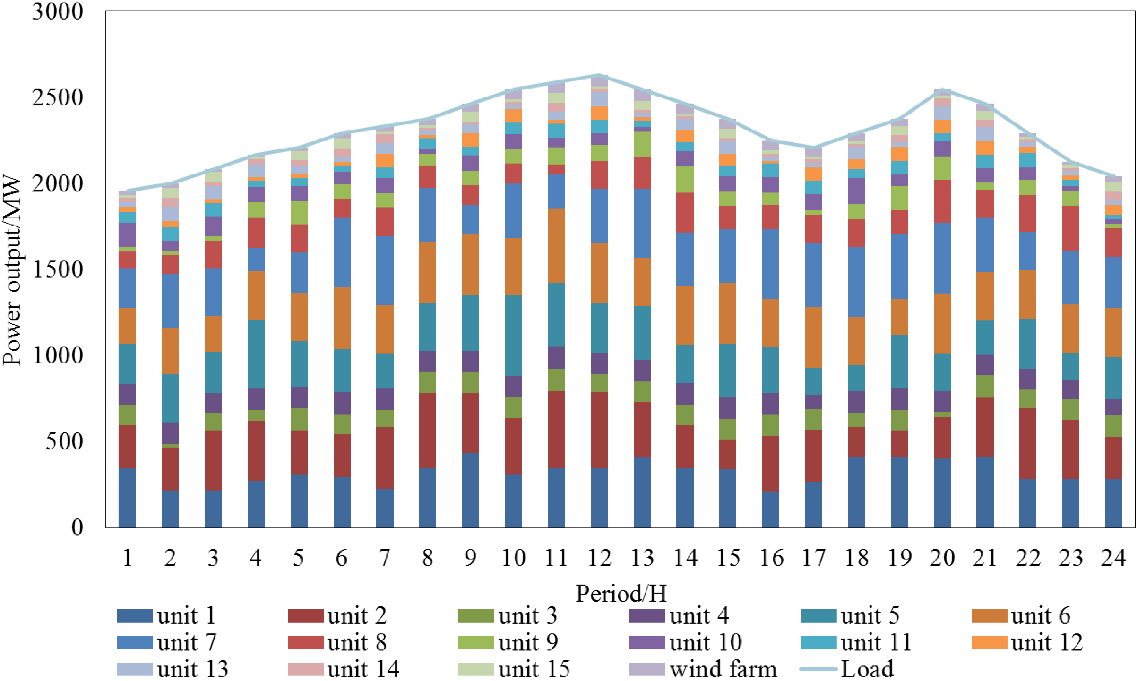
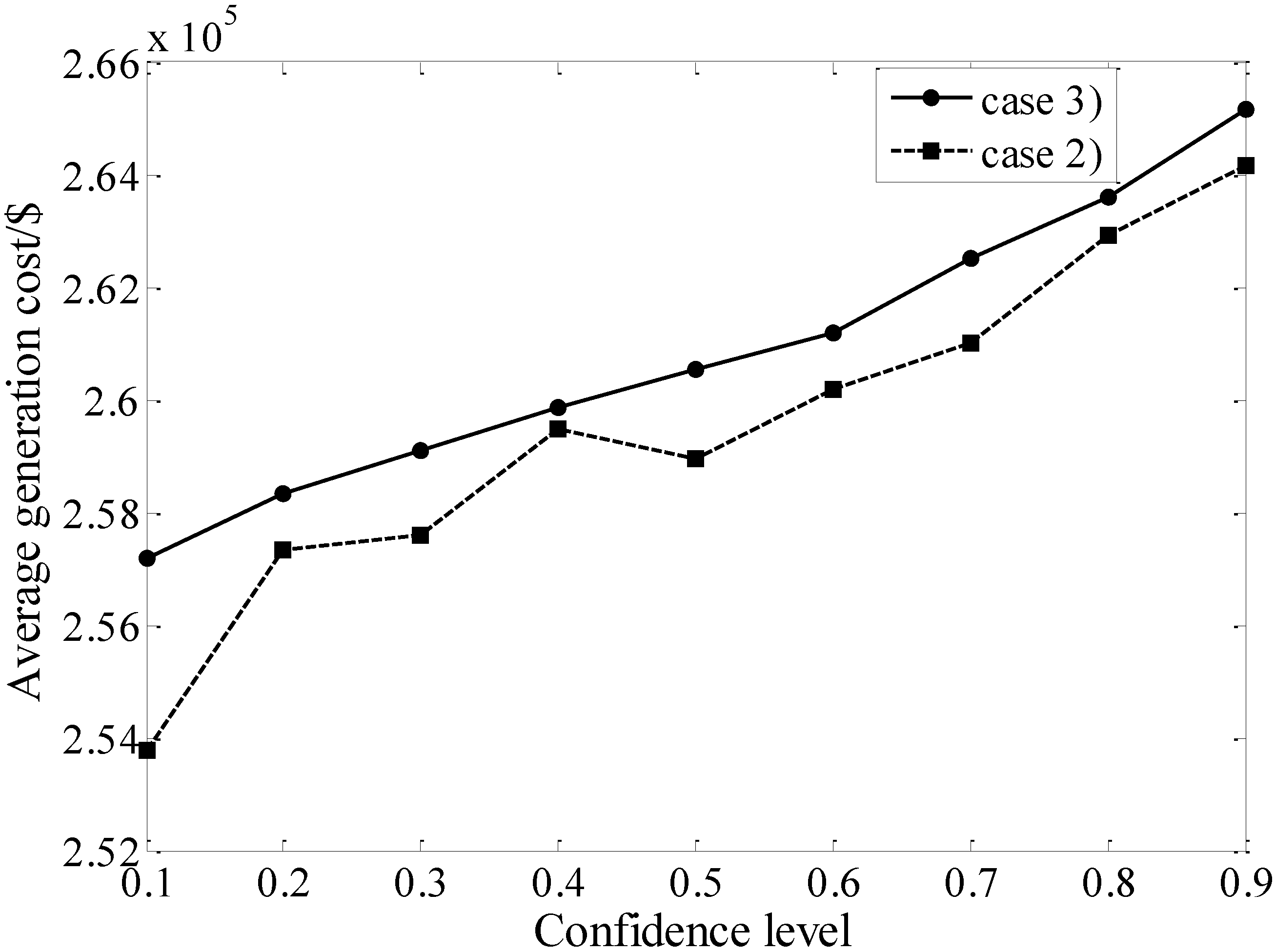
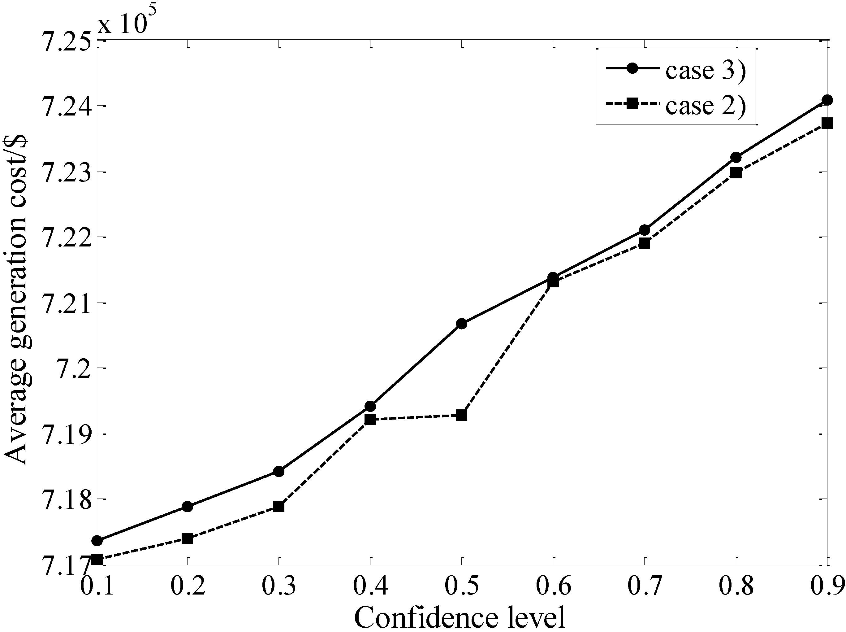
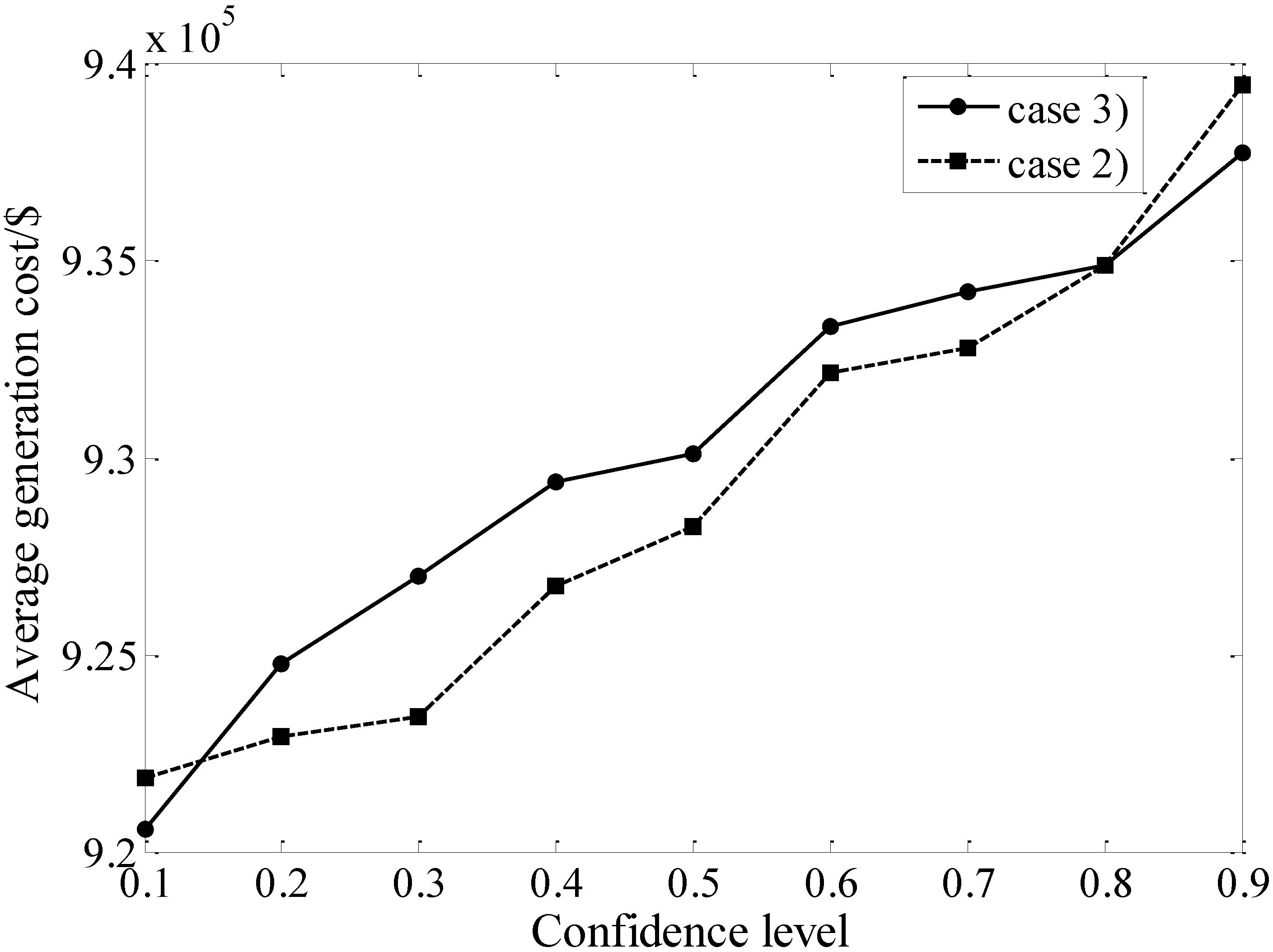
5.1. Comparisons Among the Three Cases of the DED Model

In each test system, we perform 50 trials using the improved PSO approach considering three cases as follows:

• Case (1): the DED model without considering wind power;
• Case (2): the DED model without considering wind effect in the reserve constraint;
• Case (3): the proposed DED model in this paper.

Both casea (1) and (2) can be derived from case (3). The first case can be obtained by setting the confidence level (ρ) of case (3) to 1, and the latter is obtained by removing the URFW and DRRW in the reserve constraint. Comparison results among three cases mentioned above are shown in Table 3.

Table 3. Comparisons among the three cases in the three systems.

Cases	Confidence Level	Average Generation Cost ($)
		System 1	System 2	System 3
Case (1)	1	278,903.3311	736,673.0726	952,079.3252
Case (2)	0.9	264,895.0451	723,729.9923	939,455.4055
	0.5	258,950.8628	719,280.7467	928,252.2498
	0.1	253,792.2061	717,075.4436	921,874.4037
Case (3)	0.9	265,158.6006	724,077.6842	937,747.6542
	0.5	260,537.2281	720,665.7621	930,092.0212
	0.1	257,194.5871	717,358.1034	920,580.2708

Table 3. Comparisons among the three cases in the three systems.

Cases	Confidence Level	Average Generation Cost ($)
		System 1	System 2	System 3
Case (1)	1	278,903.3311	736,673.0726	952,079.3252
Case (2)	0.9	264,895.0451	723,729.9923	939,455.4055
	0.5	258,950.8628	719,280.7467	928,252.2498
	0.1	253,792.2061	717,075.4436	921,874.4037
Case (3)	0.9	265,158.6006	724,077.6842	937,747.6542
	0.5	260,537.2281	720,665.7621	930,092.0212
	0.1	257,194.5871	717,358.1034	920,580.2708

It is evident that the average generation cost in case (1) is the highest among the three systems; this is because that no wind power is utilized in case (1). Wind power in cases (2) and (3) affords a certain proportion of the load and thus reduces the fuel consumption. Average generation cost decreases gradually as the confidence level decreases for cases (2) and (3) among the three systems. The smaller the confidence is, the lower the average generation cost is. Taking system 1 for example, the average cost in cases (2) and (3) decreases by 5.02% and 4.93%, respectively, compared to case (1) when ρ = 0.9. When ρ decreases to 0.1, the average generation cost decreases by 9.00% and 7.78%, respectively, compared to case (1).

Figure 2, Figure 3 and Figure 4 show the average cost change trend for different confidence level scenarios for cases (2) and (3) among the three systems. As seen in the figures, the average cost in the three systems increases gradually while the confidence level increases. There is not much difference in the average cost between case (3) and case (2), however, case (3) considers the URFW and DRRW in the reserve constraints, and this makes the systems more reliable.

Figure 2. Average generation cost under different confidence level in system 1.

Figure 2. Average generation cost under different confidence level in system 1.

Figure 3. Average generation cost under different confidence level in system 2.

Figure 3. Average generation cost under different confidence level in system 2.

Figure 4. Average generation cost under different confidence level in system 3.

Figure 4. Average generation cost under different confidence level in system 3.

We choose the solutions with the minimum generation cost from 50 trials as the optimal solutions by varying ρ from 0.1 to 0.9. The optimal solutions (power output during each period for each unit and wind farm) for system1 and 2 under ρ = 0.9 are shown in Figure 5 and Figure 6. Power outputs for period 1, 5, 9, 13, 17, 21 in system 3 are listed in Table 4.

Figure 5. Optimal generation output of units and wind farm in system 1 with ρ = 0.9.

Figure 5. Optimal generation output of units and wind farm in system 1 with ρ = 0.9.

Figure 6. Generation output of units and wind farm in system 2 with ρ = 0.9.

Figure 6. Generation output of units and wind farm in system 2 with ρ = 0.9.

Table 4. Optimal output of units and wind farm (WF) in system 3 with ρ = 0.9.

Unit Index	Output/MW (t = 1)	Output/MW (t = 5)	Output/MW (t = 9)	Output/MW (t = 13)	Output/MW (t = 17)	Output/MW (t = 21)
1	6.3027	2.4145	3.8440	3.1906	7.1055	6.0383
2	2.4001	3.8585	3.0919	3.8967	4.2176	4.7125
3	5.0852	2.4041	2.4051	5.3315	6.9680	5.5158
4	2.4005	2.4001	3.7132	2.4245	9.1081	5.4245
5	2.4008	2.4000	2.4001	7.7075	2.7151	2.4124
6	4.0328	9.1759	4.0017	7.5375	14.5461	7.5095
7	7.0616	4.0334	13.6143	8.2265	16.3442	6.4664
8	11.4758	4.0024	15.0108	13.5385	4.1028	8.2579
9	4.0005	4.0094	4.0025	13.9355	14.7954	4.0497
10	19.2252	47.0962	75.9820	75.9848	75.9389	52.5536
11	18.3423	55.2031	61.0610	53.5547	75.6070	31.5227
12	75.8896	15.4675	73.2103	75.9948	75.6298	53.2694
13	44.3981	62.5945	21.5289	40.1115	62.9386	75.9777
14	29.0682	78.5853	67.5916	75.0436	93.0661	91.2458
15	25.1687	25.0787	99.7008	58.6896	80.7636	69.7929
16	66.9136	25.1137	90.0044	60.3383	78.6772	97.6501
17	111.8911	54.4301	150.9160	129.1319	151.3966	102.5665
18	127.2128	91.5275	119.8840	105.7696	155.0000	148.3436
19	82.4911	81.7769	142.5084	101.8499	149.4214	104.2932
20	103.2164	84.7880	154.9953	152.8019	136.8211	102.9801
21	149.4256	79.7549	94.8661	176.8049	163.8401	167.1249
22	131.0308	142.1999	108.1115	171.1631	182.4127	84.5785
23	127.8570	125.8213	135.2337	154.7178	163.3203	153.6023
24	276.5693	158.4972	306.4523	290.2500	284.4019	287.2902
25	239.6986	270.5251	379.2529	328.7933	398.3654	331.9537
26	359.0842	372.9581	320.0320	329.1593	378.8603	275.4983
WF	19.3572	19.3837	54.5853	62.0524	63.6360	27.8695

Table 4. Optimal output of units and wind farm (WF) in system 3 with ρ = 0.9.

Unit Index	Output/MW (t = 1)	Output/MW (t = 5)	Output/MW (t = 9)	Output/MW (t = 13)	Output/MW (t = 17)	Output/MW (t = 21)
1	6.3027	2.4145	3.8440	3.1906	7.1055	6.0383
2	2.4001	3.8585	3.0919	3.8967	4.2176	4.7125
3	5.0852	2.4041	2.4051	5.3315	6.9680	5.5158
4	2.4005	2.4001	3.7132	2.4245	9.1081	5.4245
5	2.4008	2.4000	2.4001	7.7075	2.7151	2.4124
6	4.0328	9.1759	4.0017	7.5375	14.5461	7.5095
7	7.0616	4.0334	13.6143	8.2265	16.3442	6.4664
8	11.4758	4.0024	15.0108	13.5385	4.1028	8.2579
9	4.0005	4.0094	4.0025	13.9355	14.7954	4.0497
10	19.2252	47.0962	75.9820	75.9848	75.9389	52.5536
11	18.3423	55.2031	61.0610	53.5547	75.6070	31.5227
12	75.8896	15.4675	73.2103	75.9948	75.6298	53.2694
13	44.3981	62.5945	21.5289	40.1115	62.9386	75.9777
14	29.0682	78.5853	67.5916	75.0436	93.0661	91.2458
15	25.1687	25.0787	99.7008	58.6896	80.7636	69.7929
16	66.9136	25.1137	90.0044	60.3383	78.6772	97.6501
17	111.8911	54.4301	150.9160	129.1319	151.3966	102.5665
18	127.2128	91.5275	119.8840	105.7696	155.0000	148.3436
19	82.4911	81.7769	142.5084	101.8499	149.4214	104.2932
20	103.2164	84.7880	154.9953	152.8019	136.8211	102.9801
21	149.4256	79.7549	94.8661	176.8049	163.8401	167.1249
22	131.0308	142.1999	108.1115	171.1631	182.4127	84.5785
23	127.8570	125.8213	135.2337	154.7178	163.3203	153.6023
24	276.5693	158.4972	306.4523	290.2500	284.4019	287.2902
25	239.6986	270.5251	379.2529	328.7933	398.3654	331.9537
26	359.0842	372.9581	320.0320	329.1593	378.8603	275.4983
WF	19.3572	19.3837	54.5853	62.0524	63.6360	27.8695

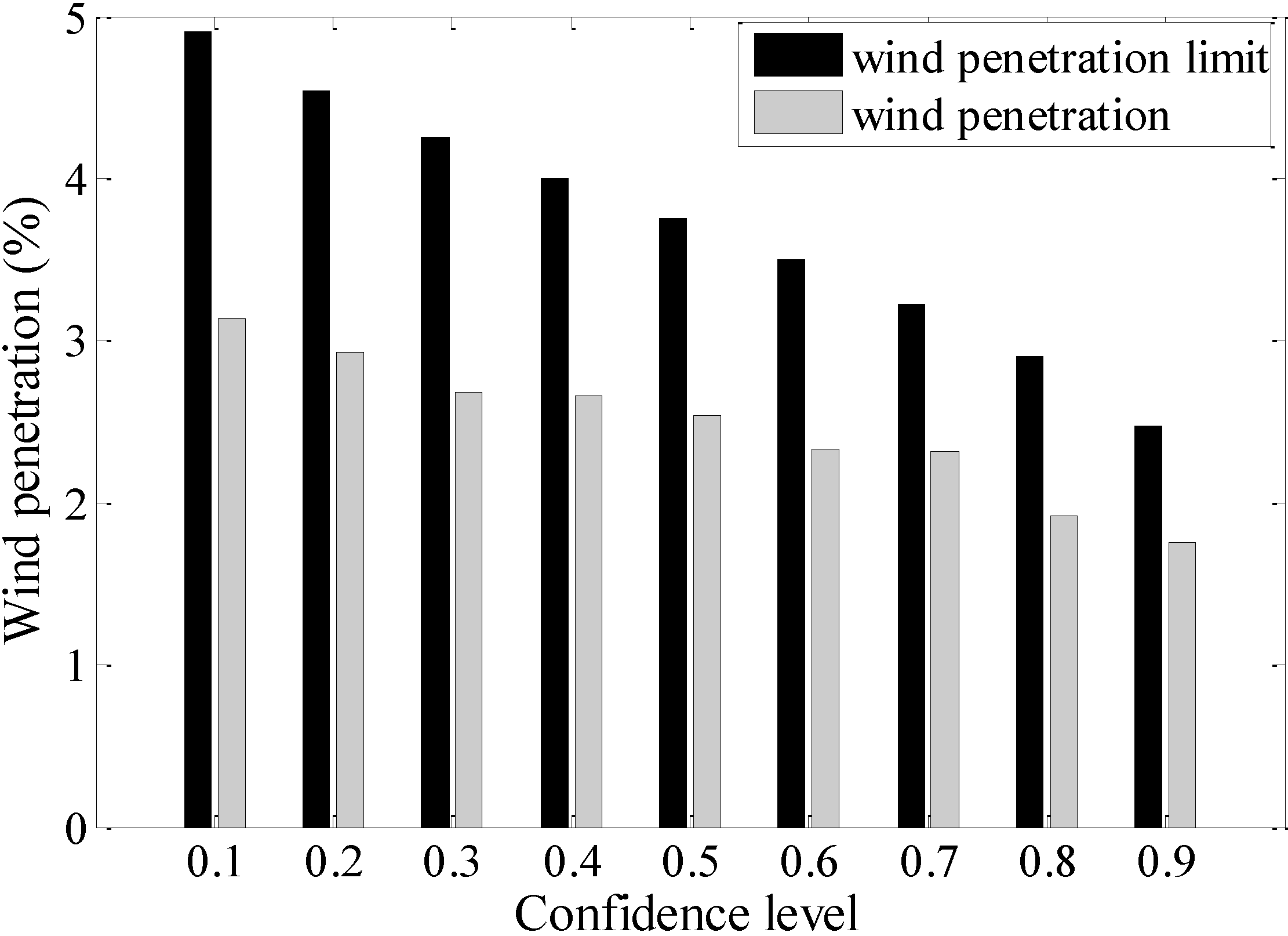
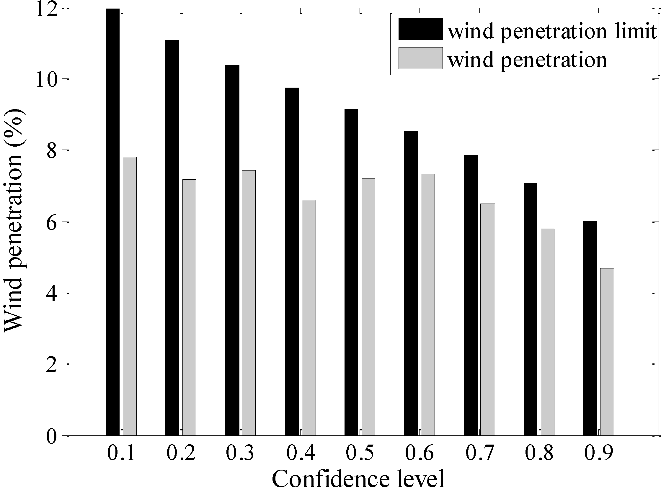
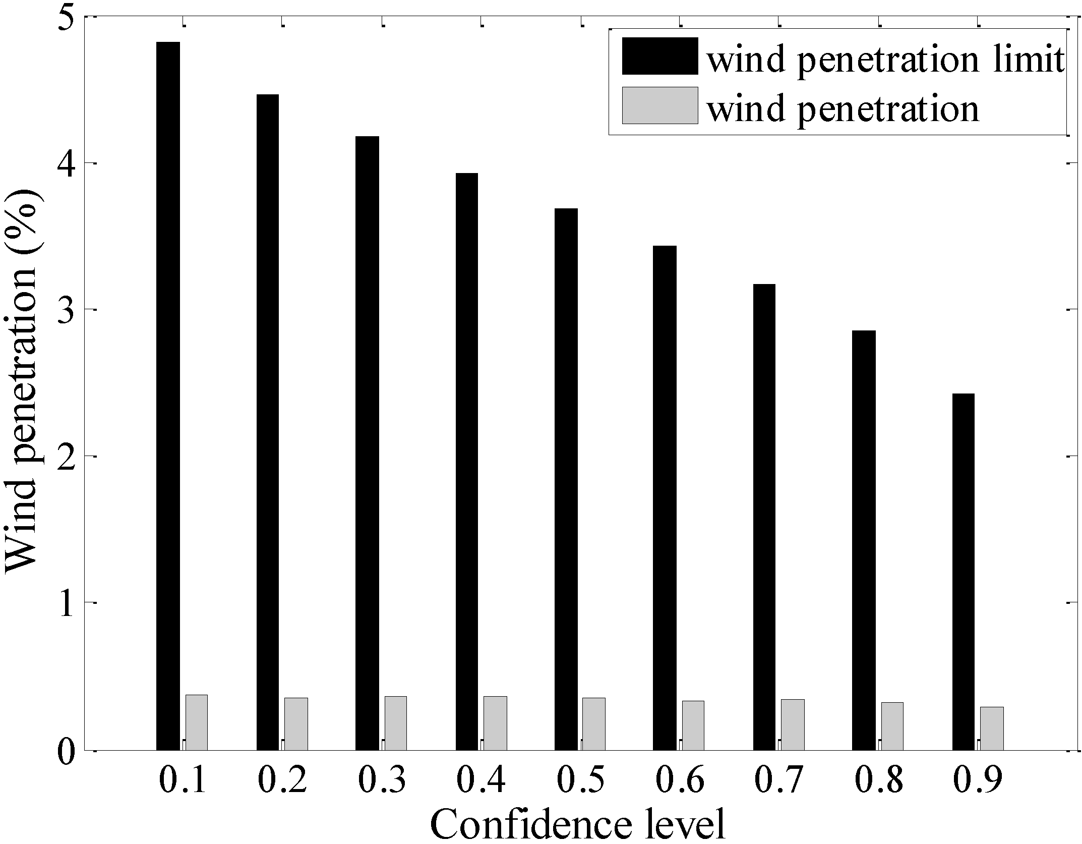
5.2. Wind Penetration as a Function of the Confidence Level Under Two Systems

Comparisons between wind penetration (${\displaystyle \sum p_{w,t}\times 100\%/{\displaystyle \sum p_{d,t}}}$) and wind penetration limits (${\displaystyle \sum w_{\text{max}}\cdot F_{X_t}^{-1}(1-\text{ρ})\times 100\%/{\displaystyle \sum p_{d,t}}}$) under the optimal solutions in each system are shown in Figure 7, Figure 8 and Figure 9. As shown, wind penetration in each system under ρ = 0.9 is the lowest, because under that situation each system requires the highest reliability and security. As the confidence level decreases, wind penetration almost increases and does not exceed the wind penetration limits in the three systems.

Figure 7. Wind penetration and its limit under different confidence levels in System 1.

Figure 7. Wind penetration and its limit under different confidence levels in System 1.

Figure 8. Wind penetration and its limit under different confidence levels in System 2.

Figure 8. Wind penetration and its limit under different confidence levels in System 2.

Figure 9. Wind penetration and its limit under different confidence levels in System 3.

Figure 9. Wind penetration and its limit under different confidence levels in System 3.

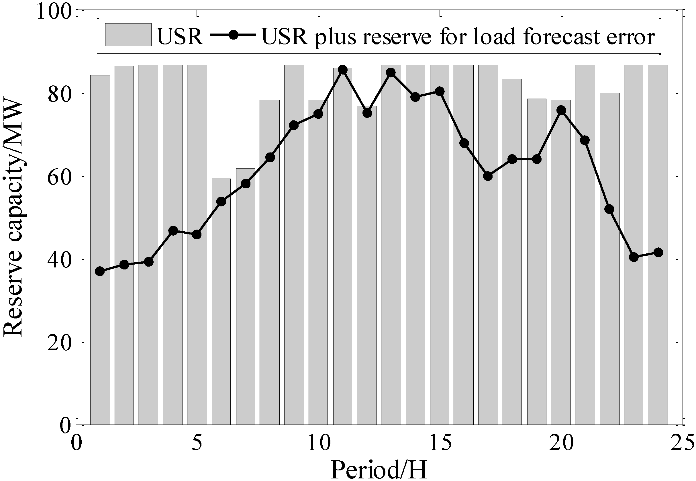
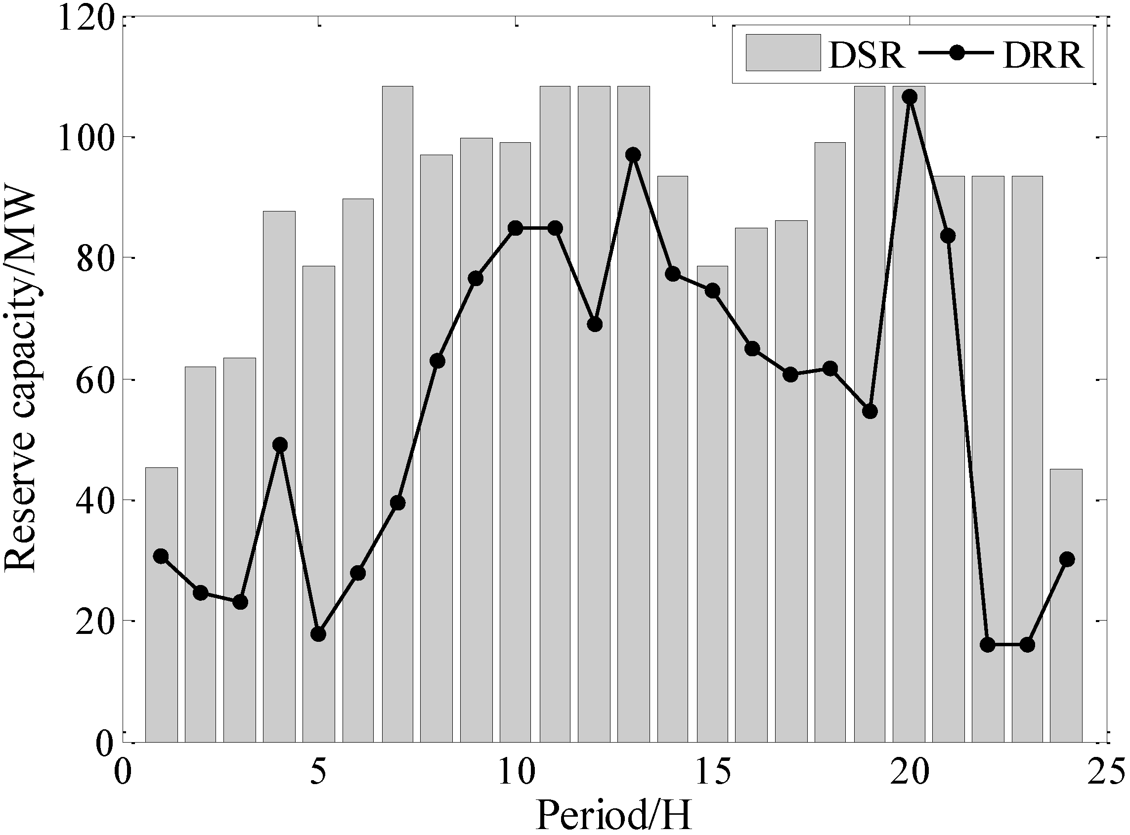
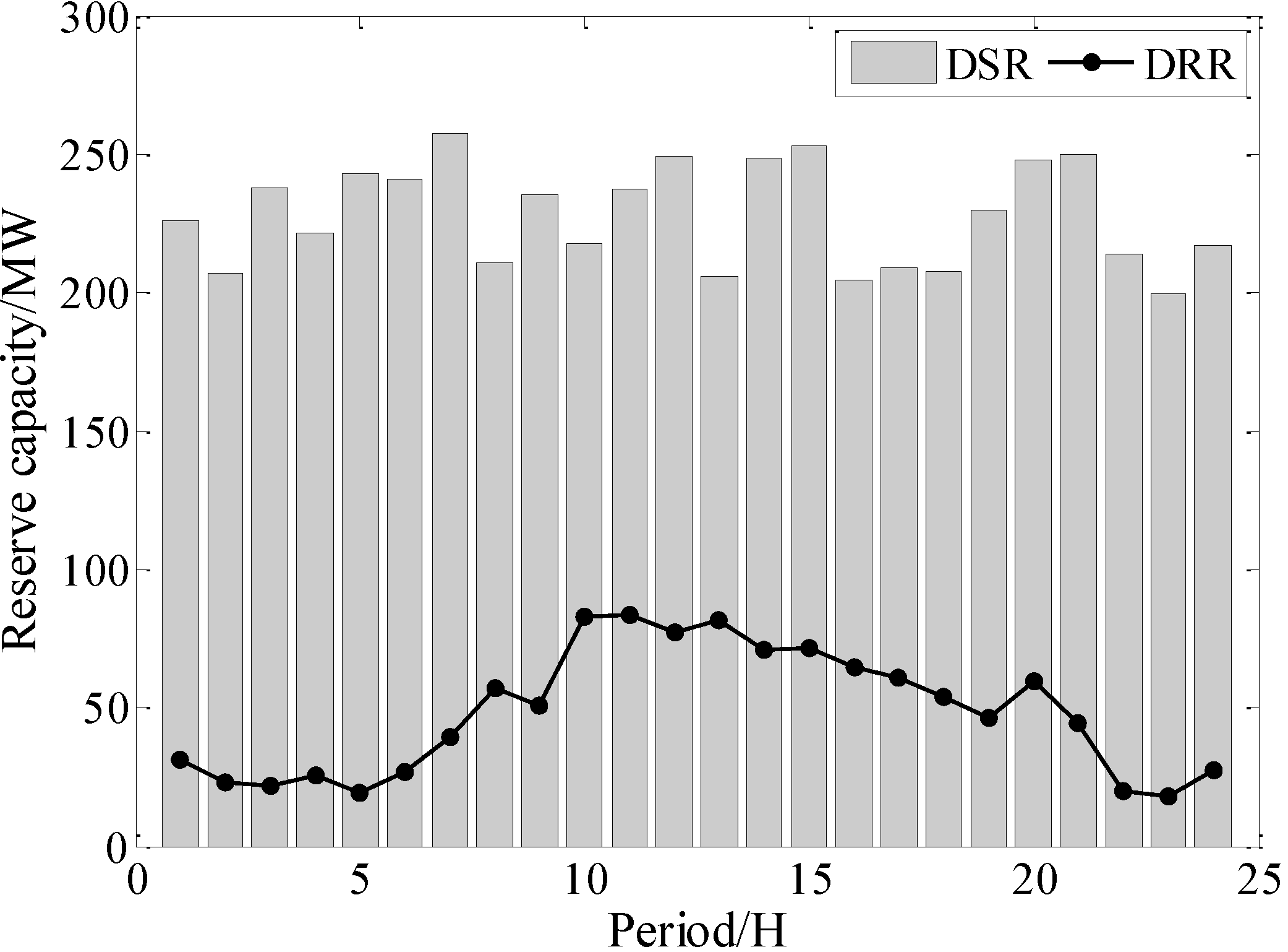
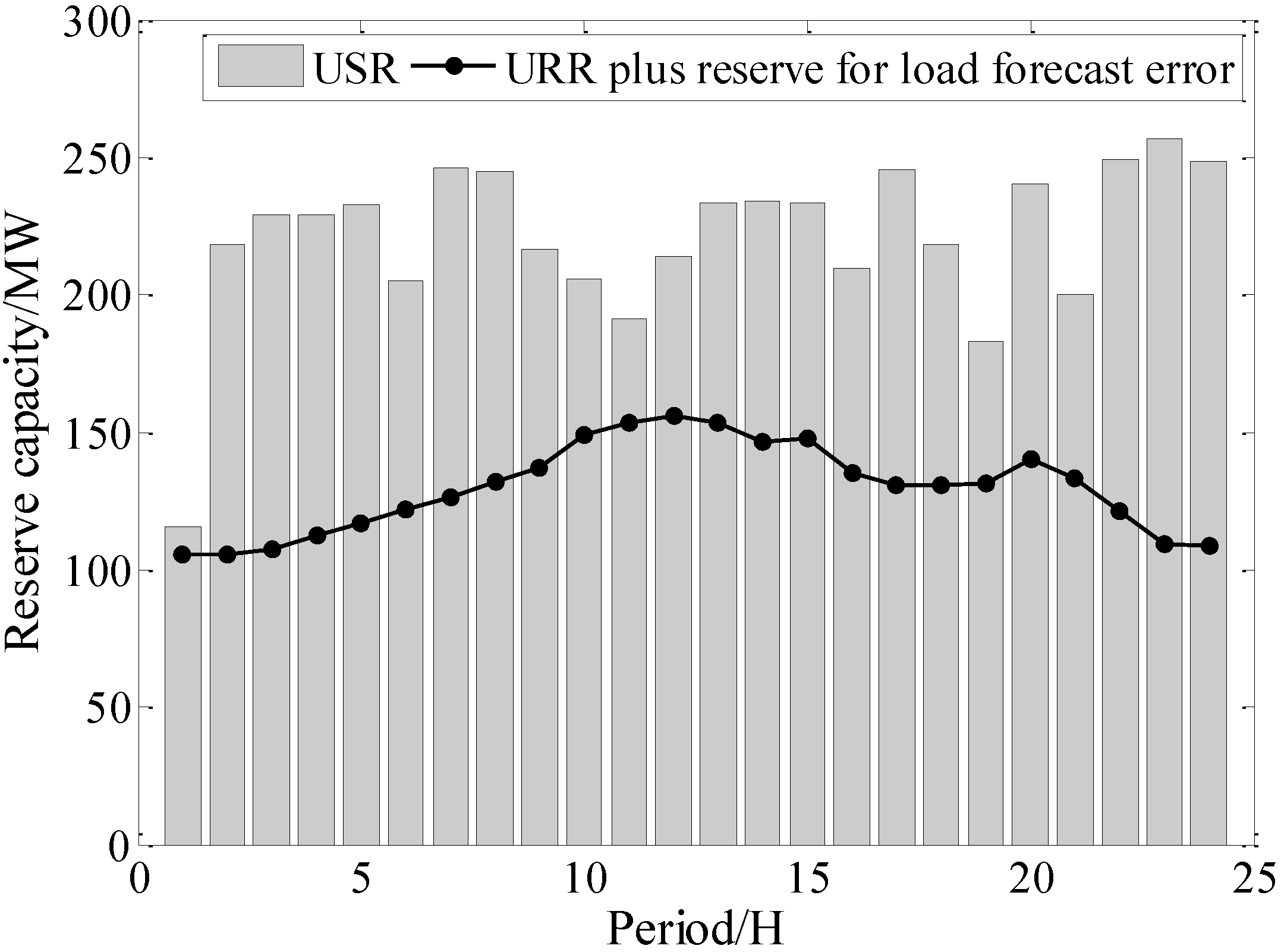
5.3. Discussion about the Optimal Reserve Allocation

Due to the stochastic and intermittent nature of wind power, the USR and DSR are used to ensure the reliability and security of systems with wind farms. According to Inequations (9) and (10), the USR, DSR, URFW and DRRW for each period are calculated based on the optimal solutions when ρ = 0.9 serves as an example. Figure 10 and Figure 11 show the optimal USR and DSR allocation for 24 h in system 1 respectively. Figure 12 and Figure 13 give the optimal USR and DSR allocation for 24 h in system 2. It can be learned that the USR and DSR provided by thermal units in both systems can effectively cover the sudden fall and increase in wind power. The same conclusion can also be drawn for system 3, so the corresponding figures for USR and DSR are not displayed.

Figure 10. The optimal USR allocation and URR plus reserve for load forecast error in system 1 with ρ = 0.9.

Figure 10. The optimal USR allocation and URR plus reserve for load forecast error in system 1 with ρ = 0.9.

Figure 11. The optimal DSR allocation and DRR for 24 h in system 1 with ρ = 0.9.

Figure 11. The optimal DSR allocation and DRR for 24 h in system 1 with ρ = 0.9.

Figure 12. The optimal USR allocation and URR plus reserve for load forecast error for 24 h in system 2 with ρ = 0.9.

Figure 12. The optimal USR allocation and URR plus reserve for load forecast error for 24 h in system 2 with ρ = 0.9.

Figure 13. The optimal DSR allocation and DRR for 24 h in system 2 with ρ = 0.9.

Figure 13. The optimal DSR allocation and DRR for 24 h in system 2 with ρ = 0.9.

5.4. Comparisons between the PSO-HCSO and PSO without HCSO

In order to investigate the effect of the parameter H on the improved PSO algorithm, we set H as 100, 200, 300, 400 and perform the algorithm on system 1 with ρ = 0.9 for 50 trials. The average generation cost and average time are listed in Table 5. The average generation costs decrease gradually and average time increases as H increases.

Table 5. Effect of H on the improved PSO algorithm with ρ = 0.9.

H	Average Generation Cost ($)	Average Time (s)
100	269,280.7296	328.2577
200	265,158.6006	386.8114
300	262,533.7753	436.2356
400	261,153.0924	538.3722

Table 5. Effect of H on the improved PSO algorithm with ρ = 0.9.

H	Average Generation Cost ($)	Average Time (s)
100	269,280.7296	328.2577
200	265,158.6006	386.8114
300	262,533.7753	436.2356
400	261,153.0924	538.3722

Finally, in order to show the effectiveness of HCSO, PSO without HCSO is used for comparison. Parameter K for PSO without HCSO is set as 300. Results of the proposed DED model under three confidence levels are shown in Table 6. Although PSO without HCSO consume less computation time than PSO-HCSO, it leads to much higher generation costs. From this point of view, the improved PSO algorithm is more efficient.

Table 6. Comparisons between PSO-HCSO and PSO without HCSO among three systems.

Approach	Confidence Level	Average Generation Cost ($)		Average Time (s)
		PSO-HCSO	PSO without HCSO	PSO-HCSO	PSO without HCSO
System 1	0.9	265,158.6006	273,039.6325	386.8114	336.6071
	0.5	260,537.2281	263,514.4852	359.3236	308.3647
	0.1	257,194.5871	262,368.0024	373.6618	317.1135
System 2	0.9	724,077.6842	731,239.0336	418.3461	409.6045
	0.5	720,665.7621	727,088.0353	402.1863	386.9233
	0.1	717,358.1034	720,196.5471	447.1164	422.8967
System 3	0.9	937,747.6542	945,013.2889	456.7289	420.0858
	0.5	930,092.0212	938,816.0995	428.3801	416.1260
	0.1	920,580.2708	929,187.2603	470.2236	436.2757

Table 6. Comparisons between PSO-HCSO and PSO without HCSO among three systems.

Approach	Confidence Level	Average Generation Cost ($)		Average Time (s)
		PSO-HCSO	PSO without HCSO	PSO-HCSO	PSO without HCSO
System 1	0.9	265,158.6006	273,039.6325	386.8114	336.6071
	0.5	260,537.2281	263,514.4852	359.3236	308.3647
	0.1	257,194.5871	262,368.0024	373.6618	317.1135
System 2	0.9	724,077.6842	731,239.0336	418.3461	409.6045
	0.5	720,665.7621	727,088.0353	402.1863	386.9233
	0.1	717,358.1034	720,196.5471	447.1164	422.8967
System 3	0.9	937,747.6542	945,013.2889	456.7289	420.0858
	0.5	930,092.0212	938,816.0995	428.3801	416.1260
	0.1	920,580.2708	929,187.2603	470.2236	436.2757

6. Conclusions

Wind power provides energy savings and environmental protection benefits. However, the intermittency and uncertainty of wind power generation require that conventional units provide additional reserve to ensure the stability and reliability of a wind power-penetrated power system. This paper formulates a DED model incorporating wind power based on CCP. The uncertain nature of wind generation is represented by a beta distribution function. In order to ensure the reliability of the power system, a chance constraint is included, and conditional expectation is presented to calculate the up and down spinning reserves. The proposed DED model is then numerically solved using an improved PSO approach in three different test systems. Results show that the proposed model can effectively respond to sudden wind power falls or raises. The improved PSO approach is fit to solve the DED model.

The results also show that the average generation cost and wind penetration are dependent on the confidence level. If the confidence level is increased, the wind penetration will be reduced, which results in higher reliability of the power system, and the average generation cost will be increased. Conversely, if the confidence level is decreased, less reliability allows more wind power to be incorporated in the power system. The average generation cost will be reduced.

References

1. Ren, B.Q.; Jiang, C.W. A review on the economic dispatch and risk management considering wind power in power market. Renew. Sustain. Energy Rev. 2009, 13, 2169–2174. [Google Scholar] [CrossRef]
2. Xia, X.; Elaiw, A. Optimal dynamic economic dispatch of generation: A review. Electr. Power Syst. Res. 2010, 80, 975–986. [Google Scholar] [CrossRef]
3. Guo, C.X.; Zhan, J.P.; Wu, Q.H. Dynamic economic emission dispatch based on group search optimizer with multiple producers. Electr. Power Syst. Res. 2012, 86, 8–16. [Google Scholar] [CrossRef]
4. Chen, C.L. Optimal wind-thermal generating unit commitment. IEEE Trans. Energy Convers. 2008, 23, 273–280. [Google Scholar] [CrossRef]
5. Zhou, W.; Peng, Y.; Sun, H.; Wei, Q.H. Dynamic economic dispatch in wind power integrated system. Proc. CSEE 2009, 29, 3–18. [Google Scholar]
6. Jiang, W.; Yan, Z.; Hu, Z. A novel improved particle swarm optimization approach for dynamic economic dispatch incorporating wind power. Electr. Power Compon. Syst. 2010, 39, 461–477. [Google Scholar] [CrossRef]
7. Hetzer, J.; Yu, C.D.; Bhattarai, K. An economic dispatch model incorporating wind power. IEEE Trans. Energy Convers. 2008, 23, 603–611. [Google Scholar] [CrossRef]
8. Zhou, W.; Sun, H.; Peng, Y. Risk reserve constrained economic dispatch model with wind power penetration. Energies 2010, 3, 1880–1894. [Google Scholar] [CrossRef]
9. Bofinger, S.; Luig, A.; Beyer, H.G. Qualification of wind power forecasts. In Proceedings of the Global Wind Power Conference, Paris, France, 2–5 April 2002; pp. 2–5.
10. Bludszuweit, H.; Dominguez-Navarro, J.A.; Llombart, A. Statistical analysis of wind power forecast error. IEEE Trans. Power Syst. 2008, 23, 983–991. [Google Scholar] [CrossRef]
11. Fabbri, A.; Roman, T.G.S.; Abbad, J.R.; Quezada, V.H.M. Assessment of the cost associated with wind generation prediction errors in a liberalized electricity market. IEEE Trans. Power Syst. 2005, 20, 1440–1446. [Google Scholar] [CrossRef]
12. Wu, D.L.; Wang, Y.; Guo, C.X.; Liu, Y. An economic dispatching model considering wind power forecast errors in electricity market environment. Autom. Electr. Power Syst. 2012, 36, 23–28. [Google Scholar]
13. Liu, X. Impact of beta-distributed wind power on economic load dispatch. Electr. Power Compon. Syst. 2011, 39, 768–779. [Google Scholar] [CrossRef]
14. Miranda, V.; Hang, P.S. Economic dispatch model with fuzzy wind constraints and attitudes of dispatchers. IEEE Trans. Power Syst. 2005, 20, 2143–2145. [Google Scholar] [CrossRef]
15. Pappala, V.S.; Erlich, I.; Rohrig, K.; Dobschinski, J. A stochastic model for the optimal operation of a wind-thermal power system. IEEE Trans. Power Syst. 2009, 24, 940–950. [Google Scholar]
16. Bouffard, F.; Galiana, F.D. Stochastic security for operations planning with significant wind power generation. IEEE Trans. Power Syst. 2008, 23, 306–316. [Google Scholar] [CrossRef]
17. Yang, N.; Wen, F. A chance constrained programming approach to transmission system expansion planning. Electr. Power Syst. Res. 2005, 75, 171–177. [Google Scholar] [CrossRef]
18. Yu, H.; Chung, C.Y.; Wong, K.P.; Zhang, J.H. A chance constrained transmission network expansion planning method with consideration of load and wind farm uncertainties. IEEE Trans. Power Syst. 2009, 24, 1568–1576. [Google Scholar] [CrossRef]
19. Wang, Q.; Guan, Y.; Wang, J. A chance-constrained two-stage stochastic program for unit commitment with uncertain wind power output. IEEE Trans. Power Syst. 2012, 27, 206–215. [Google Scholar] [CrossRef]
20. Walters, D.C.; Sheble, G.B. Genetic algorithm solution of economic dispatch with valve point loading. IEEE Trans. Power Syst. 1993, 8, 1325–1332. [Google Scholar] [CrossRef]
21. Chiang, C.L. Improved genetic algorithm for power economic dispatch of units with valve-point effects and multiple fuels. IEEE Trans. Power Syst. 2005, 20, 1690–1699. [Google Scholar]
22. Coelho, L.S.; Mariani, V.C. Combining of chaotic difference evolution and quadratic programming for economic dispatch optimization with valve-point effect. IEEE Trans. Power Syst. 2006, 22, 1273–1282. [Google Scholar]
23. Victoire, T.A.A.; Jeyakumar, A.E. Reserve constrained dynamic dispatch of units with valve-point effects. IEEE Trans. Power Syst. 2005, 22, 1273–1282. [Google Scholar] [CrossRef]
24. Chakraborty, S.; Senjyu, T.; Yona, A.; Saber, A.Y. Solving economic load dispatch problem with valve-point effects using a hybrid quantum mechanics inspired particle swarm optimization. IET Gener. Trans. Distrib. 2011, 5, 1042–1052. [Google Scholar]
25. Nidul, S.; Chakrabarti, R.; Chattopadhyay, P.K. Evolutionary programming techniques for economic load dispatch. IEEE Trans. Evol. Comput. 2003, 7, 83–94. [Google Scholar] [CrossRef]
26. Attaviriyanupap, P.; Kita, H.; Tanaka, E. A hybrid EP and SQP for dynamic economic dispatch with nonsmoooth fuel cost function. IEEE Trans. Power Syst. 2002, 17, 411–416. [Google Scholar] [CrossRef]
27. Gaing, Z.L. Particle swarm optimization to solving the economic dispatch considering the generator constraints. IEEE Trans. Power Syst. 2003, 18, 1187–1195. [Google Scholar] [CrossRef]
28. Lee, T.Y. Optimal spinning reserve for a wind-thermal power system using PSO. IEEE Trans. Power Syst. 2007, 22, 1612–1621. [Google Scholar] [CrossRef]
29. Park, J.B.; Lee, K.S.; Shin, J.R.; Lee, K.Y. A particle swarm optimization for economic dispatch with non-smooth cost functions. IEEE Trans. Power Syst. 2005, 20, 34–42. [Google Scholar] [CrossRef]
30. Li, X.H.; Jiang, C.W. Short-term operation model and risk management for wind power penetrated system in electricity market. IEEE Trans. Power Syst. 2011, 26, 932–939. [Google Scholar] [CrossRef]
31. Panigrahi, B.K.; Pandi, V.R.; Das, S. Adaptive particle swarm optimization approach for static and dynamic economic load dispatch. Energy Convers. Manag. 2008, 49, 1407–1415. [Google Scholar] [CrossRef]
32. Park, J.B.; Jeong, Y.W.; Shin, J.R.; Lee, K.Y. An improved particle swarm optimization for nonconvex economic dispatch problems. IEEE Trans. Power Syst. 2010, 25, 156–166. [Google Scholar] [CrossRef]