Optimal Scheduling of Domestic Appliances via MILP

Abstract

This paper analyzes a consumption scheduling mechanism for domestic appliances within a home area network. The aim of the proposed scheduling is to minimize the total energy price paid by the consumer and to reduce power peaks in order to achieve a balanced daily load schedule. An exact and computationally efficient mixed-integer linear programming (MILP) formulation of the problem is presented. This model is verified by several problem instances. Realistic scenarios based on the real price tariffs commercially available in the Czech Republic are calculated. The results obtained by solving the optimization problem are compared with a simulation of the ripple control service currently used by many domestic consumers in the Czech Republic.

1. Introduction

From today’s perspective, more than one hundred years have elapsed since the first time people were able to light their rooms using a switch [1]. Although the progress in many fields of science has been comparatively rapid, changes in the distribution grids proceeded only moderately. In recent years, many challenges have appeared within the energy industry. The power demand has reached new peak levels and created special requirements on balancing electricity demand and generation. Moreover, economic and environmental reasons will cause distribution companies to consider more complex power balance scenarios [2], and currently, it is also believed that the next generation power grid will be green in terms of the environmental impact. At present, such systems are generally known as smart grids.

The smart grid system is defined as “the use of sensors, communications, computational ability and control in some form to enhance the overall functionality of the electric power delivery system. A dumb system becomes smart by sensing, communicating, applying intelligence, exercising control and through feedback, continually adjusting. For a power system, this permits several functions which allow optimization in combination with the use of bulk generation and storage, transmission, distribution, distributed resources and consumer end uses toward goals which ensure reliability and optimize or minimize the use of energy, mitigate environmental impact, manage assets, and contain cost” [3].

The development of a smart grid does not involve replacing the existing electricity network, because such a process would be impossible for technical and economical reasons. The entire concept is rather based on an enhancement of the actual network via implementing new services and features, a procedure in which the old physical infrastructure is to be maintained to the highest possible degree [4].

According to a related report of the European Commission [5], households use 26.7% of the total energy generated. The distribution of such a large amount of energy places significant requirements on the distribution grid. Moreover, the consumption has a highly fluctuating character (depending on the time of day, the day of the week or the season) with daily-based, repeating power demand peaks. Such peaks impose additional requirements on the distribution grid. Two general approaches to optimize the use of energy by domestic end users are consumption reduction and consumption shifting [6]. While the former notion can be achieved by increasing consumer awareness or via constructing energy efficient buildings (e.g., houses with better thermal insulation), the latter one means deferring the cycle of the most demanding appliances from peak to off-peak hours. The aim of consumption shift is to reduce the peak-to-average ratio.

The demand-side management (DSM) approach proposed in the 1980s is a modification of user-generated energy demand preferences performed to optimize overall energy consumption [7]. One of the most fundamental requirements for the DSM is consumption shifting (thus, for example, electric water heater warming or electric vehicle charging can be carried out during late night or early morning hours, namely when there is much less demand than in the peak period). Less intensive requirements on the grid facilitate an increase in the energy delivery stability and grid lifetime, and they reduce the need of massive investment in the grid hierarchy.

It is obvious that the initial cost of such systems will not be negligible and that a substantial part of the expenditures will have to be borne by domestic users [8]. A well-designed system of incentives must be introduced to increase user willingness to initial investment; relevant stimuli can be materialized, for example, in the form of dynamic or real-time pricing [9].

Related Work: The entire demand scheduling problem has been examined by many authors; however, we mainly focus on studies utilizing the (mixed) integer linear programming approach. Even though our research is based on the model proposed by paper [2], several changes were carried out, including optimization by removing a set of redundant decision variables. This step then led to the simplification of the problem. Moreover, the possibility of enlarging the model to comprise several dwellings has been introduced, and, as mentioned below, a number of minor changes have also been performed. The work in [7] describes the employment of the MILP to schedule product manufacturing consumption for an industrial consumer. The work in [10] then discusses the given problem with respect to the use of electricity and heat storage; here, however, less emphasis is placed on the appliance running cycle definition. While [11,12] consider predominantly the optimization of finding the trade-off between cost reduction and minimization of the waiting time to start the appliances, the research report [13] discusses the optimization of both various appliance classes (e.g., schedulable and interruptible appliances) and heat comfort with respect to cost reduction. By further extension, [14] presents the consumption scheduling mechanism based on integer linear programming, but it does not consider the time fluctuating price tariff. The work in [15] analyzes the problem of electrical load management in smart homes via the evolutionary algorithms, and [16] solves the energy production and consumption optimization issue by means of heuristics. An appliance scheduling framework for residential consumers that exploits reinforcement learning is introduced in [17].

The following portion of this paper is organized as follows: The mathematical model is defined and described in Section 2. Several models of dwellings and case studies are introduced in Section 3. Section 4 presents the computational results defined in Section 3. The conclusions and discussion are provided in Section 5.

2. Demand-Side Consumption Scheduling

2.1. System Description

The model presented in this section is used to solve the problem of optimal scheduling of domestic appliances. This model was inspired by the approach proposed in [2] and constitutes an enlarged variant enabling us to optimize the consumption of more than one dwelling. Moreover, several model constraints were changed (e.g., the restriction on the assignment of energy phase power), which leads to the elimination of the set of real decision variables and changes the problem to the binary integer linear program. The computational complexity remains, nevertheless, the same as in the original problem: namely, NP hard. After such a modification of the constraints, the model better fits the input data format.

The system describes a set of dwellings containing multiple domestic appliances whose working cycles are divided into sequentially executed energy phases. An energy phase is considered to be an uninterruptible sub-task of appliance operation and also a basic scheduling unit. All of the phases are described by their length, total power consumption and peak power consumption. The phases determined for a single appliance are run sequentially. Several additional constraints can be defined for each phase, including the maximum execution time and the maximum inter-phase delay for every two phases.

Besides the constraints defined by the appliance manufacturer, there are several other limitations. The total power provided by the grid is restricted, and this limit cannot be exceeded during the whole scheduling interval. Moreover, various user-defined time preferences can be specified, allowing certain appliances to run only within particular time intervals (e.g., between 8:00 and 14:00). We also considered unmanageable appliances (i.e., devices that cannot be scheduled by the energy coordinator). These appliances can be either added to the model with fixed processing time or considered a part of the base load, which is defined here as the set of the energy and peak power values for each time slot. Our model allows scheduling a set of dwellings together. Furthermore, each dwelling may include a different subset of appliances.

In Table 1 below, all symbols used within the optimization model are described. Generally, the small letters represent the decision variables, and the capital letters substitute the constants. The decision variables are denoted by the subscripts (e.g., x_h,i,j,k = 1, which indicates that the i − th appliance in the h − th dwelling processes its j − th phase in the time slot k). The model constraints are organized into several groups: power constraints, timing constraints and user constraints.

Table 1. Model symbols.

Symbol	Description
	Indices and model size
h	Dwelling index
i	Appliance index
j	Energy phase index
k	Time slot index
H	Number of dwellings
I	Number of appliances
J	Maximal number of power phases defined for each appliance
K	Number of scheduled time slots
	Decision variables
xh,i,j,k	Binary variable; one if the phase j in the appliance i in the dwelling h is running in the time slot k
yh,i,j,k	Binary variable; one if the phase j in the appliance i in the dwelling h is already finished in the time slot k
zh,i,j,k	Binary variable; one if the phase j in the appliance i in the dwelling h is waiting for run in the time slot k
	Constants (let Ψ = H · I)
PT	Processing time of all appliance classes and power phases (Ψ × J )
PC	Power consumed by all appliance classes during the power phases (Ψ × J )
PP	Peak power of all appliance classes during the power phases (Ψ × J )
PD	Maximum allowed waiting time for the next phase if the previous one is finished for all appliances and their phases (Ψ × J )
AH	Matrix of the presence of appliances in the dwellings ( H × I). Note that this matrix determines the instantiation of the appliance classes to concrete dwellings.
UP	User preference matrix (Ψ × K). A value of one states that the appliance i in the dwelling h can be scheduled in the time slot k
UC	Appliances consequence matrix (Ψ × Ψ). A value of one states that the appliance i1 in the dwelling h1 must finish its cycle before the appliance i2 in the dwelling h2 starts.
Θ	Energy price vector
Pmax	Peak power
Pbase	Vector of the household base load caused by unmanageable devices

Table 1. Model symbols.

Symbol	Description
	Indices and model size
h	Dwelling index
i	Appliance index
j	Energy phase index
k	Time slot index
H	Number of dwellings
I	Number of appliances
J	Maximal number of power phases defined for each appliance
K	Number of scheduled time slots
	Decision variables
xh,i,j,k	Binary variable; one if the phase j in the appliance i in the dwelling h is running in the time slot k
yh,i,j,k	Binary variable; one if the phase j in the appliance i in the dwelling h is already finished in the time slot k
zh,i,j,k	Binary variable; one if the phase j in the appliance i in the dwelling h is waiting for run in the time slot k
	Constants (let Ψ = H · I)
PT	Processing time of all appliance classes and power phases (Ψ × J )
PC	Power consumed by all appliance classes during the power phases (Ψ × J )
PP	Peak power of all appliance classes during the power phases (Ψ × J )
PD	Maximum allowed waiting time for the next phase if the previous one is finished for all appliances and their phases (Ψ × J )
AH	Matrix of the presence of appliances in the dwellings ( H × I). Note that this matrix determines the instantiation of the appliance classes to concrete dwellings.
UP	User preference matrix (Ψ × K). A value of one states that the appliance i in the dwelling h can be scheduled in the time slot k
UC	Appliances consequence matrix (Ψ × Ψ). A value of one states that the appliance i1 in the dwelling h1 must finish its cycle before the appliance i2 in the dwelling h2 starts.
Θ	Energy price vector
Pmax	Peak power
Pbase	Vector of the household base load caused by unmanageable devices

2.2. Consumption Scheduling Optimization

$${\displaystyle \sum _{h=1}^H{\displaystyle \sum _{i=1}^I{\displaystyle \sum _{j=1}^{J}P{P}_{i,j}}}}\cdot x_{h,i.j.k}\le P_{\mathit{\text{max}}}-p_{bas{e}_k}\forall k$$

(1)

$$x_{h,i,j,k}\le A{H}_{h,i}\forall h,i,j,k$$

(2)

Equation (1) defines the peak power boundaries for all appliances and time slots. The total power will not exceed the P_max− P_base value, which represents the non-schedulable consumption. Equation (2) then allows enabling or disabling a certain appliance in a certain dwelling.

$${\displaystyle \sum _{k=1}^K{x}_{h,i,j,k}}=P{T}_{i,j}\forall h,i,j$$

(3)

$$x_{h,i,j,k-1}-x_{h,i,j,k}\le y_{h,i,j,k}\forall h,i,j,k:k>1$$

(4)

$$x_{h,i,j,k}\le y_{h,i,j-1,k}\forall h,i,j,k:j>1$$

(5)

$${\displaystyle \sum _{k=1}^K{z}_{h,i,j,k}}⪯P{D}_{i,j}\forall h,i,j$$

(6)

Equation (3) ensures that the processing time of each power phase will not exceed the amount specified by the parameter PT. According to Equation (4), a power phase is uninterruptible since its beginning. The sequential processing of all phases within one appliance is ensured by Equation (5). Once a particular phase (except for the last one in the appliance cycle) is finished, the following phase is started either immediately or after an interphase delay (Equation (6)). The symbol ⪯ can be substituted by = (the delay assumes exactly the given PD value) or by ≤ (when the delay is shorter or equal to the PD value).

$$x_{h,i,j,k}\le U{P}_{i,k}\forall i,j,k$$

(7)

$$U{C}_{i1,i2}\cdot x_{h,i2,1,k}\le y_{h,i1,J,k}\forall h,i_1,i_2,k:i_1,i_2\in \mathrm{1..}I$$

(8)

Equation (7) states that the appliances can be scheduled only during their allowed time intervals described in the matrix UP . The user may need to schedule a subgroup of appliances as a chain (e.g., the second appliance is scheduled after the first one has been finished). Equation (8) applies the consequence rules defined in the matrix UC. If we have UC_i1,i2 = 1 for any two appliances i₁ and i₂, then (for every time slot k) the appliance i₂ cannot perform its first power phase if the last power phase of the appliance i₁ has not been finished yet. Moreover, for all i₁ and i₂, there must hold UC_i1,i2 + UC_i2,i1 ≤ 1.

$$x_{h,i,j,k}\le 1-y_{h,i,j,k}\forall h,i,j,k$$

(9)

$$y_{h,i,j,k-1}\le y_{h,i,j,k}\forall h,i,j,k:k>1$$

(10)

$$z_{h,i,j,k}=y_{h,i,j-1,k}-x_{h,i,j,k}-y_{h,i,j,k}\forall h,i,j,k:j>1$$

(11)

$$x_{h,i,j,k}\in \left\{0,1\right\};y_{h,i,j,k}\in \left\{0,1\right\};z_{h,i,j,k}\in \left\{0,1\right\}\forall h,i,j,k$$

(12)

The last block of equations describes the implementation rules. These rules ensure the expected behavior of the model. Equation (9) states that once the phase has been finished, it cannot jump into the running state anymore, and it is obvious from Equation (10) that the finished phase cannot be performed again. The interphase delay mechanism is provided by Equation (11). The constraints 12 state that all of the decision variables are binary.

2.3. Objective Function

The optimization of the proposed model is performed to minimize the total price of the electricity consumed by the domestic appliances. The price in the criterial function is represented as the vector Θ. The objective function is then:

$${\displaystyle \sum _{k=1}^K({\mathrm{\Theta }}_k\cdot {\displaystyle \sum _{h=1}^H{\displaystyle \sum _{i=1}^I{\displaystyle \sum _{j=1}^{J}P{C}_{i,j}}}}\cdot x_{h,i,j,k}))}$$

(13)

2.4. Problem Formulation

The MILP problem described in 14 is a classical optimization paradigm and can be solved using algorithms, such as the branch-and-bound method.

$$\begin{array}{c}\underset{x,y,z}{\min }\text{\hspace{1em}objective function (13)}\\ \text{subject to constraints (1-12)}\end{array}$$

(14)

3. Case Study

Several linear programming solvers are currently available. As a rule, non-commercial solvers (e.g., CBC [18], LPSOLVE [19], SCIP [20] or GLPK [21]) do not exhibit such computational efficiency as commercial ones (e.g., GUROBI [22], CPLEX [23] or the MATLAB optimization toolbox [24]). All of the experiments were performed using the CPLEX 12.6 MILP solver, which is freely accessible for academic applications. The computer was equipped with a 2.4 GHz Intel(R) Core(TM) i7-3630 QM processor and 8 GB of RAM, and the computational time required to find the optimal solution fluctuated between 180 and 240 s for 100 variations of the model.

In this section, we report on a set of computational experiments performed under different scenarios with varying tariffs, and we present several examples of energy scheduling optimization within 24 h. The scheduling interval is divided into 96 time slots; each of these slots lasts 15 min. Hence, a quarter-hour is the smallest scheduling time unit.

The study involves six dwellings and six types of domestic appliances, a structure partially inspired by [25]. The appliances used in the model are washing machines (WM), dishwashers (DW), tumble dryers (TD), electronic water heaters (EWH), electric ovens (EO) and home lighting subsystems (HL). We determined the set of appliances present in each dwelling (Table 2) as the mapping of the saturation value obtained from [26,27]. For the EWH, we considered a 50% presence rate, because we intended to compare two groups of customers with significantly different energy consumption values. The resulting binary integer linear program consists of 103,680 binary variables. Note that the same problem adjusted to the model from [2] comprises a further 34,561 real decision variables. Although this was not originally intended, the simplification reduces the solving time by approximately 10%.

Table 2. Presence of the appliances (washing machines (WM), dishwashers (DW), tumble dryers (TD), electronic water heaters (EWH), electric ovens (EO) and home lighting subsystems (HL)) in the dwellings.

Identifier	Saturation	Dwelling						Cycles per year
		1	2	3	4	5	6
WM	0.97	✓	✓	✓	✓	✓	✓	220
DW	0.66	✓	✓	✓	✓			240
TD	0.42	✓	✓					147
EWH	0.50	✓		✓		✓		328
EO	0.85	✓	✓	✓	✓	✓		182
HL	1.00	✓	✓	✓	✓	✓	✓	330

Table 2. Presence of the appliances (washing machines (WM), dishwashers (DW), tumble dryers (TD), electronic water heaters (EWH), electric ovens (EO) and home lighting subsystems (HL)) in the dwellings.

Identifier	Saturation	Dwelling						Cycles per year
		1	2	3	4	5	6
WM	0.97	✓	✓	✓	✓	✓	✓	220
DW	0.66	✓	✓	✓	✓			240
TD	0.42	✓	✓					147
EWH	0.50	✓		✓		✓		328
EO	0.85	✓	✓	✓	✓	✓		182
HL	1.00	✓	✓	✓	✓	✓	✓	330

The calculation for each dwelling and price tariff was performed 100 times with variable input parameters, such as appliance run demands and user preferences. The number of cycles per year for the appliances was obtained from several sources; the WM, DW and TD values were acquired from reference [28]. The EWH and HL cycle count allows for the number of vacation days and public holidays in the Czech Republic. The EO cycle count is experimentally set to 50%, and the probability that the appliance is run during the particular day can be obtained as P = cycles_per_year/365.

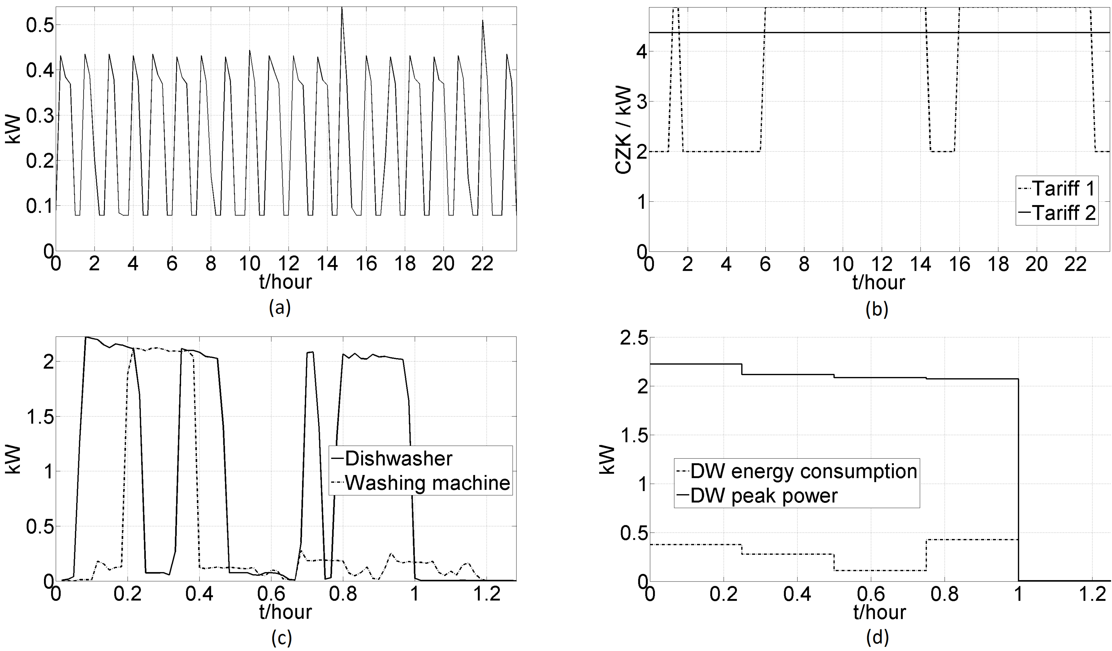
For the WM, DW, TD and EO, the real energy profiles were measured and the discrete substitutions calculated. The EWH characteristic was estimated by the electrical characteristics of a common domestic water heater and hot water consumption in an average household. The HL time behavior was evaluated based on the data shown in [29]. In each appliance, the energy consumed for each time slot was calculated as (1/t) ·${\displaystyle \sum p}$, where t is the time slot length and p is the vector of instantaneous power values measured within the defined interval. The peak power values for each time slot were obtained as max (p). We used an energy consumption logger with the period of one minute, and the calculated values for all the domestic appliances and their phases are presented in Table 3. The real power profiles for the DW and WM appliances are shown in Figure 1c, while the discrete-time values for the DW calculated by the introduced procedure are presented in Figure 1d.

The model facilitates the reduction of the maximum power consumed by all of the domestic appliances. As most customers in the Czech Republic who use electric water heaters have satisfactory technical infrastructure, we do not consider any restriction of the peak power value. However, from the provider’s point of view, domestic users can be encouraged (by either rewards or penalties) to meet criteria even stricter than those given by technical limitations. Such incentives, however, are not analyzed in this study.

For comparison purposes, we consider two price tariffs that are extended to form three different problems in total. Each of these problems is solved for six dwellings, and there are 100 instances calculated for each dwelling. The following paragraphs describe the above-mentioned tariffs and models; relevant solutions to the problems are shown in detail in Section 4.

Table 3. Appliance energy profiles.

ID	Phase length	Energy per phase/kWh	Peak per phase/kW
WM	5 × 1	0.15, 0.29, 0.03, 0.03, 0.02	2.12, 2.12, 0.28, 0.26, 0.18
DW	6 × 1	0.38, 0.28, 0.11, 0.43, 0.01, 0.01	2.23, 2.12, 2.09, 2.07, 0.01, 0.01
TD	6 × 1	0.15, 0.20, 0.20, 0.20, 0.17, 0.01	2.20, 2.20, 2.20, 2.20, 2.20, 0.10
EWH	9 × 2	2 × [0.90, 0.90, 0.85, 0.85] 1, 0.81	2 × [1.80, 1.80, 1.75, 1.75], 1.80
EO	6 × 1	0.44, 0.24, 0.17, 0.15, 0.27, 0.01	1.84, 1.88, 1.88, 1.89, 2.18, 0.01
HL	4 × 8, 4	0.01, 0.02, 0.05, 0.02, 0.01	0.04, 0.08, 0.19, 0.06, 0.04

¹ The section in brackets is repeated twice.

Table 3. Appliance energy profiles.

ID	Phase length	Energy per phase/kWh	Peak per phase/kW
WM	5 × 1	0.15, 0.29, 0.03, 0.03, 0.02	2.12, 2.12, 0.28, 0.26, 0.18
DW	6 × 1	0.38, 0.28, 0.11, 0.43, 0.01, 0.01	2.23, 2.12, 2.09, 2.07, 0.01, 0.01
TD	6 × 1	0.15, 0.20, 0.20, 0.20, 0.17, 0.01	2.20, 2.20, 2.20, 2.20, 2.20, 0.10
EWH	9 × 2	2 × [0.90, 0.90, 0.85, 0.85] 1, 0.81	2 × [1.80, 1.80, 1.75, 1.75], 1.80
EO	6 × 1	0.44, 0.24, 0.17, 0.15, 0.27, 0.01	1.84, 1.88, 1.88, 1.89, 2.18, 0.01
HL	4 × 8, 4	0.01, 0.02, 0.05, 0.02, 0.01	0.04, 0.08, 0.19, 0.06, 0.04

¹ The section in brackets is repeated twice.

Figure 1. (a) Base load; (b) pricing tariffs; (c) real DW and WM profiles; (d) discrete form of DW peak and energy.

Figure 1. (a) Base load; (b) pricing tariffs; (c) real DW and WM profiles; (d) discrete form of DW peak and energy.

Tariff 1: The first selected option was the commercially available flat tariff D02d, one of the most widespread tariffs in the Czech Republic. This tariff is offered by most electricity distributors (e.g., [30,31,32]). For this article, we follow unit electricity prices granted by the E.ON provider [30]. The constant unit price comprises the cost of electricity, transmission charge, capacity charge, taxes and other items (e.g., the distributed energy resource or OTE support [33]); the assumed value is 4.37 CZK per kWh.

Tariff 2: The second selected option was another commercially available tariff, namely the D25d, from the same provider. According to [30], the two price levels offered within this tariff are 4.88 CZK and 1.99 CZK per kWh with ripple control (RC) service [34]. In this paper, we used the service identifier A1B8DP6 valid for the region of southern Moravia. More details on both tariffs are indicated in Figure 1b.

Instance S1: Due to the constant price and no power limit restriction, the scheduling scheme does not have to be applied. The total price per day can be calculated as the sum of the consumed energy and the unit price. For clarity, we use the scheduling algorithm and show that the solution leads to the latest starting time run of all appliances. This case is taken as the reference for all other instances.

Instance S2, Tariff 2 with ripple control: The RC coordinator is used to switch the EWH automatically when the low price level is applied. The remaining white appliances are assumed to be run within short intervals in the evenings. We focused on comparing the total energy price with Instance S1, which indicates the cost reduction that can be reached via ripple control.

Instance S3, Tariff 2 with optimal scheduling: The ripple control coordinator device is replaced with a more sophisticated coordinator, which can control not only the EWH, but also the other domestic appliances according to the user-defined criteria. The aim is to evaluate the cost reduction granted by this instance compared to that offered by S2.

4. Results

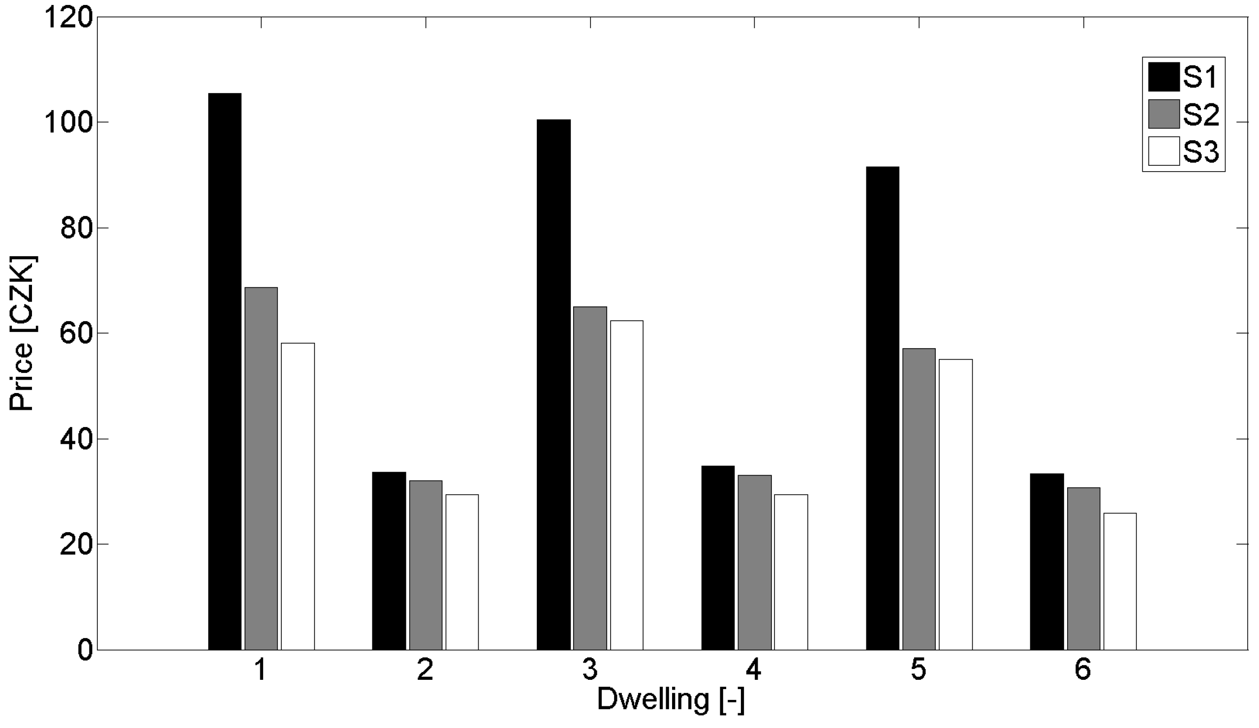
The absolute calculated prices and relative expense cuts for all of the dwellings are shown in Table 4 and Figure 2. The results for each dwelling were obtained as average values taken from all 100 calculated instances.

Instance S1: Table 4 suggests a significantly higher energy consumption rate and total energy price consumed by Dwellings 1, 3 and 5. These dwellings consume electricity to heat water (Table 2), while Dwellings 2, 4 and 6 use electricity only for common appliances. The saturation of these appliances has only a minor impact on the total electricity price.

Table 4. Average energy consumed.

Dwelling	Absolute price (CZK)			Relative cuts (%)
	S1	S2	S3	S1→S2	S2→S3	S1→S3
1	105.4	68.6	58.1	34.9%	15.3%	44.8%
2	33.6	32.1	29.4	4.7%	8.2%	12.5%
3	100.5	65.0	62.4	35.3%	4.0%	37.9%
4	34.8	33.1	29.4	5.1%	11.1%	15.6%
5	91.5	57.1	55.0	37.7%	3.7%	39.9%
6	33.3	30.7	25.9	7.9%	15.6%	22.2%

Table 4. Average energy consumed.

Dwelling	Absolute price (CZK)			Relative cuts (%)
	S1	S2	S3	S1→S2	S2→S3	S1→S3
1	105.4	68.6	58.1	34.9%	15.3%	44.8%
2	33.6	32.1	29.4	4.7%	8.2%	12.5%
3	100.5	65.0	62.4	35.3%	4.0%	37.9%
4	34.8	33.1	29.4	5.1%	11.1%	15.6%
5	91.5	57.1	55.0	37.7%	3.7%	39.9%
6	33.3	30.7	25.9	7.9%	15.6%	22.2%

Instance S2: The dwellings that use electricity to heat water significantly reduce their consumption and cost of energy by using the ripple control system. This saving fluctuates around 35% compared to S1 (Table 4); for the other dwellings, the cost reduction oscillates between 4 and 8%. Such a difference then confirms the fact that RC service is suitable, especially for consumers who use electric water heaters. However, using a tariff with the ripple control system is conditioned by the satisfaction of strict criteria. As one of these criteria consists in the necessity to use an accumulative electric water heater [30], it is obvious that the ripple control system becomes very beneficial in this case.

Figure 2. Average energy consumed.

Figure 2. Average energy consumed.

Instance S3: In general, the optimal scheduling of domestic appliances facilitates additional electricity price cuts compared to the ripple control system; this cost reduction is given mainly by the optimized run of all domestic appliances, not only the EWH. The resulting values are shown in columns S1→S3 and S2→S3 of Table 4. Since the consumption of the other domestic appliances (WM-DW-TD, etc.) is low compared to that shown by the EWH, columns S2→S3 indicate lower reduction values than rank S1→S2.

Recapitulation: The current electricity market and tariffs in the Czech Republic do not offer any major price cuts above the level of those obtainable with the present ripple control system. Considering the sum of money that must be invested to implement the smart appliance optimal scheduling system, it is obvious that the entire implementation process cannot be profitable; however, broader usage of distributed energy resources and plug-in hybrid electric vehicles (PHEV) would probably change this conclusion.

4.1. Scheduling Algorithm Verification

In this section, the functionality of the scheduling algorithm is described. We model a group of six dwellings, each with six appliances mentioned in Table 2. All of these dwellings are controlled together by one scheduling device within one day. Generally, all of the involved appliances are present in all of the dwellings, and their switching preferences are set to the same values, as described in Table 5. We consider two cases for the optimization. In the first case (labeled as Instance C1), we perform the optimization with respect to the total price of consumed electrical energy in the same manner as in the previous chapter. In the second case (labeled as Instance C2), there is also the maximal power restriction applied. The value of this restriction is set to 7,360 watts. This value corresponds to the current of 32 A, which is the double of the nominal value of the main circuit breaker for many customers.

Table 5. Appliance run behavior both for non-scheduled and scheduled cases.

Identifier	Type	W/O scheduling	With scheduling
WM	Shiftable	16:00 to 21:00	8:00 to 16:00
DW	Shiftable	18:00 to 22:00	8:00 to 16:00
TD	Shiftable	18:00 to 22:00	8:00 to 16:00, after WM cycle
EWH	Thermostatic	starts at 20:00	0:00 to 23:59
EO	Non-shiftable	19:00 to 20:30	18:00 to 19:30 1
HL	Non-shiftable	06:00 to 08:30	16:00 to 23:00 2

¹ The preferences of electric oven users allow only a single running time a day; ² To observe the MILP problem formulation, the home lighting system is modeled as an appliance, which starts at 6:00; the two peak periods during the day are modeled as two phases with an exact interphase delay time.

Table 5. Appliance run behavior both for non-scheduled and scheduled cases.

Identifier	Type	W/O scheduling	With scheduling
WM	Shiftable	16:00 to 21:00	8:00 to 16:00
DW	Shiftable	18:00 to 22:00	8:00 to 16:00
TD	Shiftable	18:00 to 22:00	8:00 to 16:00, after WM cycle
EWH	Thermostatic	starts at 20:00	0:00 to 23:59
EO	Non-shiftable	19:00 to 20:30	18:00 to 19:30 1
HL	Non-shiftable	06:00 to 08:30	16:00 to 23:00 2

¹ The preferences of electric oven users allow only a single running time a day; ² To observe the MILP problem formulation, the home lighting system is modeled as an appliance, which starts at 6:00; the two peak periods during the day are modeled as two phases with an exact interphase delay time.

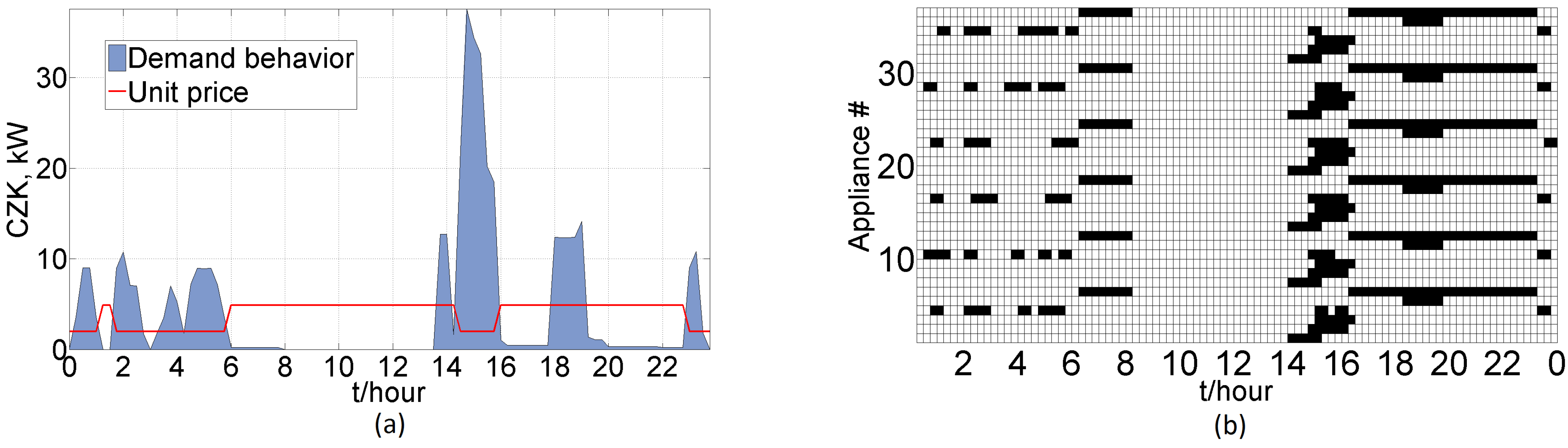
Results of Instance C1: The peak value is not constrained, and therefore, the power demand during the low price cycle reached 35 kW (Figure 3a). The scheduling plan in Figure 3b indicates that all of the manageable appliances, with the sole exception of the washing machines, are scheduled to low price level intervals. (Each row of the scheduling plan describes one appliance. There are six appliances in six dwellings; thus, Rows 1–6 describe the WM-DW-TB-EO-EWH-HL appliances of the first dwelling, Rows 7–12 appliances of the second dwelling, etc. The columns correspond to 15-min intervals (time slots). The black square means that the specific appliance is run in the specific time slot.) In the optimization problem, the WMs must finish their cycles before the TDs can be run. The EOs are run between 18:00 and 20:00, thus causing the second most significant demand peak; this fact, together with the home lighting consumption cycle, obviously cannot be eliminated.

Figure 3. (a) C1 price and energy consumed; (b) scheduling plan.

Figure 3. (a) C1 price and energy consumed; (b) scheduling plan.

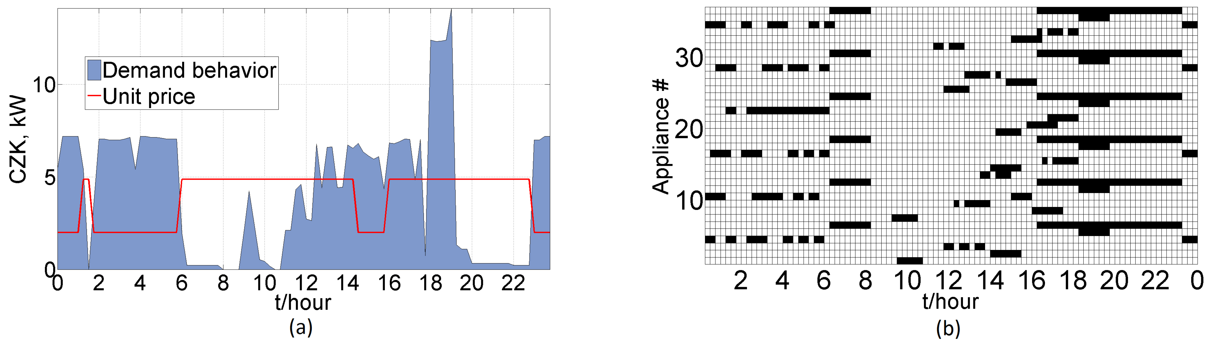
Results of Instance C2: For the bounded variant of the scheduling problem, the peak value of the power demand does not exceed the defined power level for most of the day (Figure 4a). The value of 12 kW was reached only when all of the installed electric ovens (EO) were run together, namely during the interval between 18:00 and 19:30. This situation corresponds to the group of users preparing dinner after coming back home from work; the EOs are therefore classified as unmanageable appliances. Figure 4b presents the scheduling plan for the consecutive pattern of the WM-DW-TD appliance cycles in all of the dwellings.

Figure 4. (a) C2 price and energy consumed; (b) scheduling plan.

Figure 4. (a) C2 price and energy consumed; (b) scheduling plan.

Table 6 summarizes both optimization results. The total price is noticeably lower in Instance C1 than in C2. Here, the optimization problem is solved without the maximal power restriction. All of the unmanageable appliances can thus be scheduled also to the low price level tariff. However, significant demand peaks occur in this case. On the other hand, for the given problem, Instance C2, the demand peaks are reduced to below the boundary value of 7,360 watts. The total electricity price for the discussed problem is 12% higher compared to C1. This is caused by the fact that a portion of the appliances must be run during the high price cycle. The last column of Table 6 shows the time spent by the solver on obtaining the solution, and it is obvious that Instance C2 can be described as significantly more demanding in this respect than C1.

Table 6. Scheduling algorithm verification results.

Instance	Tariff	Constraints	Total price	Max. peak	Solving time
C1	Tariff 2	No	290 CZK	34 kW	18 s
C2	Tariff 2	7360 Watts	325 CZK	14 kW (7 kW)	80 s

Table 6. Scheduling algorithm verification results.

Instance	Tariff	Constraints	Total price	Max. peak	Solving time
C1	Tariff 2	No	290 CZK	34 kW	18 s
C2	Tariff 2	7360 Watts	325 CZK	14 kW (7 kW)	80 s

The longer solution period typical of Instance C2 is due to the fact that the stricter the constraints, the more difficult the processing. For C2, the stricter constraints are caused by the total power limit.

5. Conclusions and Future Work

This paper describes the theory and implementation of a linear model to define and schedule smart appliances within one or more dwellings. The model was designed as a mixed integer linear problem implemented in the ILOG CPLEX development environment and solved by the CPLEX solver. The primary optimization criterion is the total electricity price within specific requirements. These can involve not only the user preferences or technical limits of the appliances, but also the maximal peak power value restriction. We verified the functionality of the model by two application cases, where the energy consumption for six dwellings was optimized.

We employed the discussed model to investigate the possibility of cost reduction for various customers that use different groups of domestic appliances. We created six dwellings, each with a specific group of predefined appliances; for each dwelling, 100 instances were generated according to pre-set criteria. All of the given problems were solved for two tariffs offered in the Czech Republic. The flat price tariff was compared with the ripple control tariff, for which we prepared two scenarios. Generally, the first scenario was based on the RC system, and the second one utilized the model and optimal scheduling. The above-mentioned cases were all compared from the perspective of the total energy price. In this context, we then analyzed the fundamental question of whether the optimal scheduling of home appliances could bring any further cost reduction to surpass the current ripple control system. According to the results shown in Section 4, additional cost cuts of 3%–16% were reached. However, the sum of the calculated price reduction appears to be insufficient when compared with the amount of investment necessary to set up the smart system. Until the offered electricity price tariffs change significantly or fluctuating tariffs with reasonable peak and non-peak price differences are introduced, it will not be beneficial for a typical domestic customer to seek a solution more mature and complex than the ripple control system.

The planned research activities include extending the model with the possibility of distributed generation from renewable power sources and electricity storage (e.g., PHEV batteries). We also intend to optimize the consumption of both electric energy and gas within a single model. There are nevertheless many other interesting problems to be considered with respect to the cogeneration by µCHP, heat storage or heat consumption.

From the formal point of view, proposed extensions comprise the multi-criteria optimization problem and, most importantly, a non-linear stochastic model to be used instead of the linear-deterministic case. Hence, we plan to design and implement the model by means of stochastic programming.