Dynamic Feedforward Control of a Diesel Engine Based on Optimal Transient Compensation Maps

Abstract

To satisfy the increasingly stringent emission regulations and a demand for an ever lower fuel consumption, diesel engines have become complex systems with many interacting actuators. As a consequence, these requirements are pushing control and calibration to their limits. The calibration procedure nowadays is still based mainly on engineering experience, which results in a highly iterative process to derive a complete engine calibration. Moreover, automatic tools are available only for stationary operation, to obtain control maps that are optimal with respect to some predefined objective function. Therefore, the exploitation of any leftover potential during transient operation is crucial. This paper proposes an approach to derive a transient feedforward (FF) control system in an automated way. It relies on optimal control theory to solve a dynamic optimization problem for fast transients. A partially physics-based model is thereby used to replace the engine. From the optimal solutions, the relevant information is extracted and stored in maps spanned by the engine speed and the torque gradient. These maps complement the static control maps by accounting for the dynamic behavior of the engine. The procedure is implemented on a real engine and experimental results are presented along with the development of the methodology.

1. Introduction

In recent years, due to increasingly stringent emission regulations [1,2] and ever more challenging goals in terms of fuel economy improvement, and reduction of noise and vibration, the complexity of engine systems has proportionally increased. New technologies help to fulfill such demanding requests, but they come at a price. The increased complexity and the exploitation of the entire hardware potential introduce two important subjects, which are optimal engine calibration and transient control. The aim of the present work is to merge these two requirements, or rather to apply the optimal control theory to achieve an incisive transient control. Static optimization of the control inputs of an engine is the first step towards the calibration of an engine control unit. This optimization can be carried out directly on the real engine [3] or by utilizing models to represent the engine [4,5]. The number of actuations influencing the engine performance is increasing, and, as a consequence, the effort in the calibration of control parameters can be very costly and demanding. Often, with the aim of speeding up the calibration process several methodologies can be applied, for example, statistical tools [6] or automatic calibration procedures carried out along engine transients [7,8]. The resulting steady-state maps usually constitute the first step to parameterize the engine control unit in form of a feedforward (FF) control structure. Without any further manipulation, this kind of control system cannot capture dynamic phenomena, leading to high emission peaks and fuel inefficiency during transient operation. An alternative approach could take into account engine dynamics through mathematical models, in order to implement a model-based rapid transient calibration optimization process [9].

In this paper, we propose to account for the dynamic behavior of the engine by transient FF control. In order to derive a transient controller, engine modeling for control purposes is the first step. Hence, control oriented models (COM) of engines have been presented in several works [1,10,11,12]. Although many COMs have been developed for the purpose of transient control of different types of engines, deriving accurate physics-based models, which cover the whole engine operating region, is a difficult and not always successfully achievable task [13]. For this reason, our approach relies on a custom-tailored model that is valid in a region around the actual state and input trajectories. With the difficulties in estimating engine responses, transient control of engines can be realized by using FF controls, based on steady-state actuator set-point maps, and transient compensation maps. However, generating suitable compensation maps for transient operation is of crucial importance, and this role often relies more on engineering experience than on engine physics, resulting in a highly iterative calibration process, which is not systematically repeatable and provides only suboptimal results.

This paper focuses on this topic, and presents the numerical methods and the testbench setup to derive optimal transient compensation maps, implementable in a FF control structure. The proposed approach is characterized by a combination of physics-based and set-point relative mathematical models, in synergy with optimal control of diesel engines [14,15].

Firstly, the main concept behind this work is presented in ; the optimization-oriented modeling of diesel engines is summarized in ; subsequently the dynamic optimization methodology and related numerical methods are described in , including a brief description of the experimental setup in ; the presentation of results, in , focuses on the effectiveness of the methodology and shows some side aspects potentially interesting; finally, the experimental validation provided in demonstrates the meaningfulness of the approach.

2. Methods

The experimental activity has been carried out on a light-duty engine that is used mainly in EU4 C-segment passenger car. It is a 3.0 l V6 diesel engine, equipped with a common-rail injection system, a high pressure cooled exhaust gas recirculation (EGR) circuit and a variable geometry turbine (VGT) turbocharger (TC) (Table 1). While the EGR valve positioning has an intuitive convention, as EGR = 0% means fully closed and no gas recirculation, a clarification for the VGT position might be useful for the reader. In the given control system, a VGT position = 100% corresponds to a fully closed condition, and vice versa the distributor is fully open with a VGT position = 0%. In other words, when the VGT is fully closed (100%) it means that the turbine, under steady state flow conditions, generates the highest backpressure correspondent to that mass flow rate, and therefore the pressure drop through the turbine is maximum. In this condition, the turbine produces its maximum power, increasing the TC speed, with the consequent increase of the intake manifold (IM) pressure.

Table 1. Main data of the engine used in this work. EGR: exhaust gas recirculation; VGT: variable geometry turbine; TC: turbocharger; and CDI: common-rail diesel injection.

Engine type	Diesel, V6
Displacement	2987 cm3
EGR	high pressure, cooled
Compression ratio	15.5
TC	VGT, charge-air cooler
Bore/stroke	83/92 mm
Injection	CDI 4, maximum 1600 bar
Valves/cylinder	4
Maximum torque	400 N·m (1400–3800 rpm)
Rated power	165 kW (3800 rpm)

Table 1. Main data of the engine used in this work. EGR: exhaust gas recirculation; VGT: variable geometry turbine; TC: turbocharger; and CDI: common-rail diesel injection.

Engine type	Diesel, V6
Displacement	2987 cm3
EGR	high pressure, cooled
Compression ratio	15.5
TC	VGT, charge-air cooler
Bore/stroke	83/92 mm
Injection	CDI 4, maximum 1600 bar
Valves/cylinder	4
Maximum torque	400 N·m (1400–3800 rpm)
Rated power	165 kW (3800 rpm)

2.1. The Concept

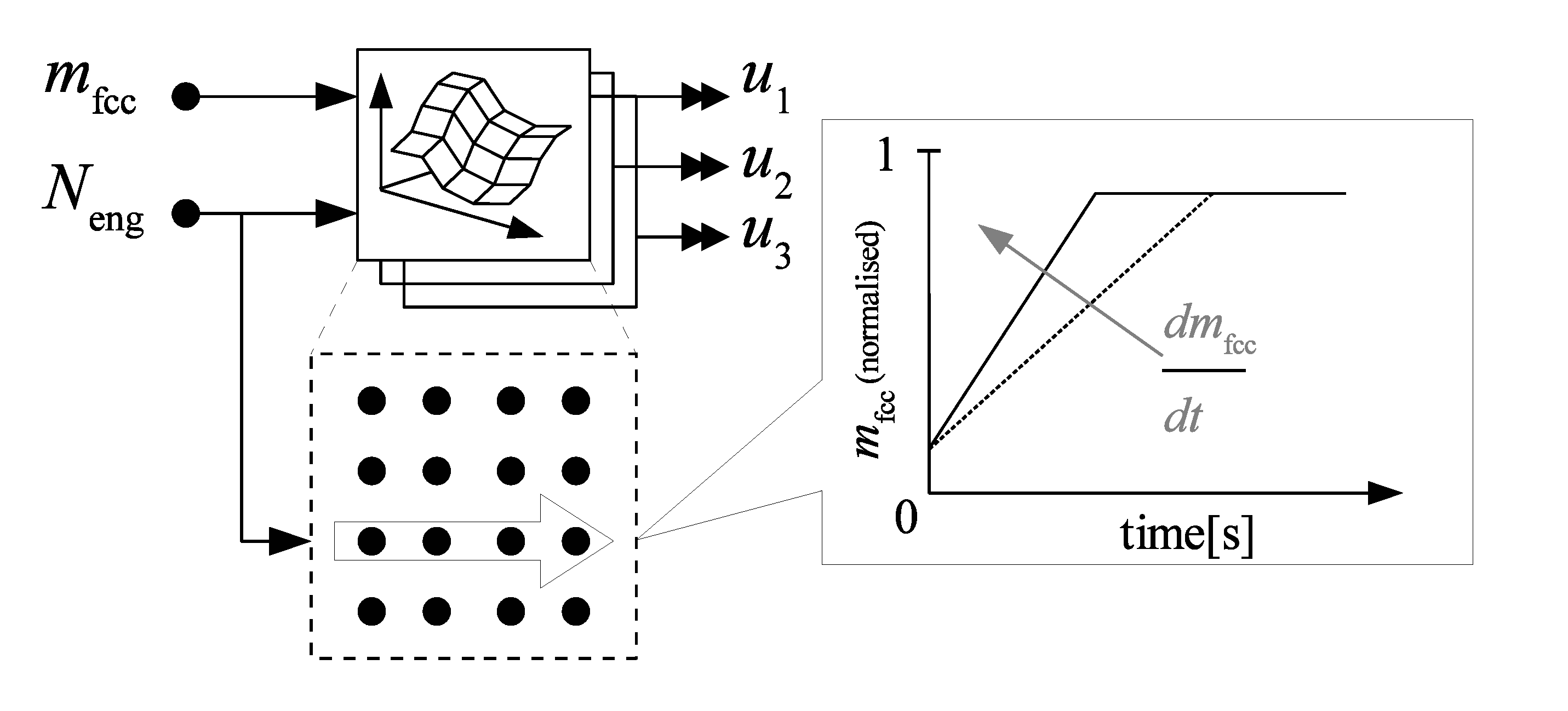
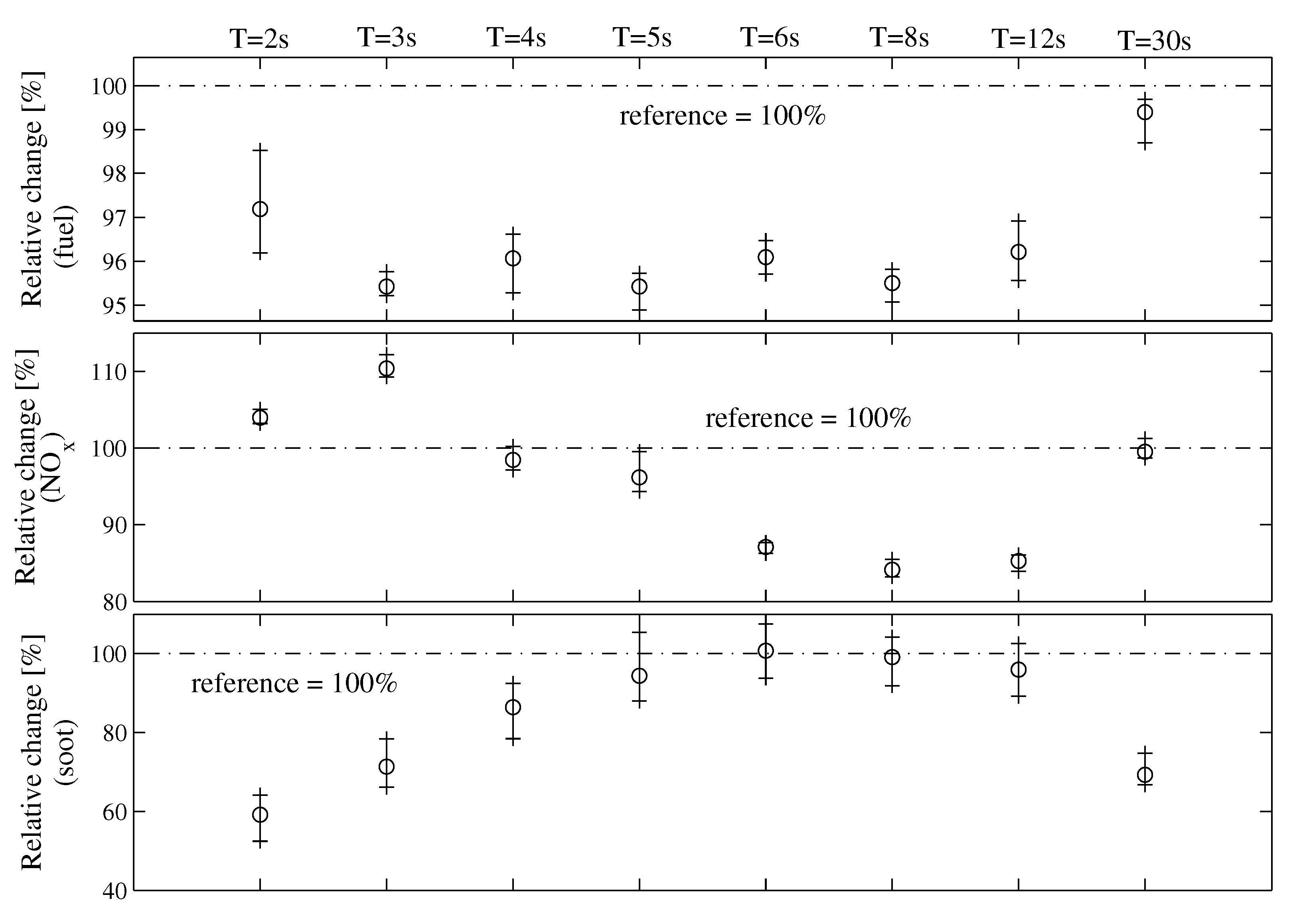
The top left corner of Figure 1 shows a typical FF control structure based on steady-state control maps, spanned by engine speed (N_eng) and load (m_fcc). In a diesel engine, if neither torque limitation nor smoke limitation are active, the load request directly corresponds to a specific fuel quantity injected per cycle in each cylinder (m_fcc). To investigate the typical dynamic behavior of the engine, load transients at constant engine speed are performed by operating the engine over load ramps, and the results are analyzed in terms of fuel consumption and emissions. 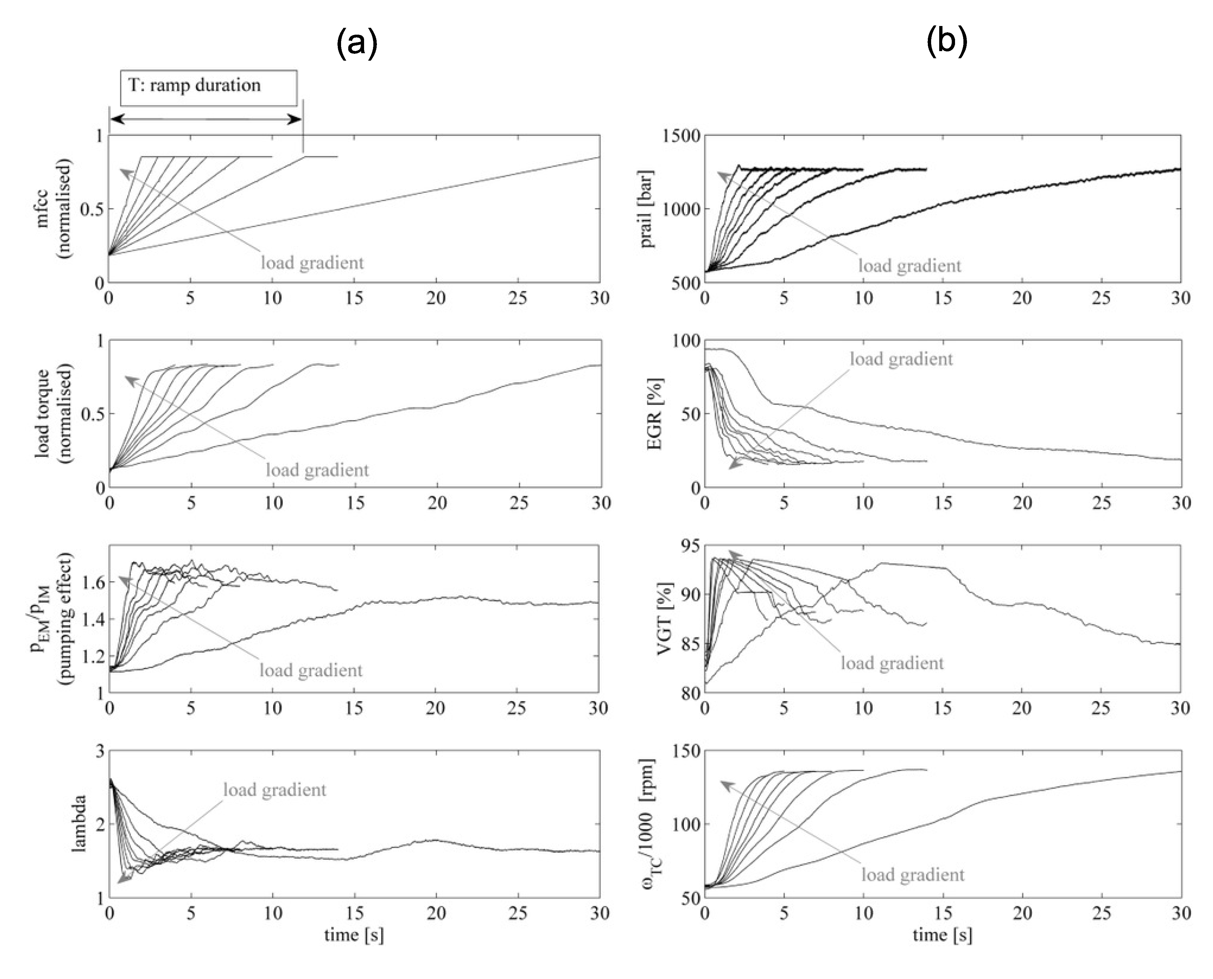With the aim of exploring the entire load range, fuel ramps from 10% to 85% of maximum load and with different durations, have been carried out on the testbench (see Figure 1). 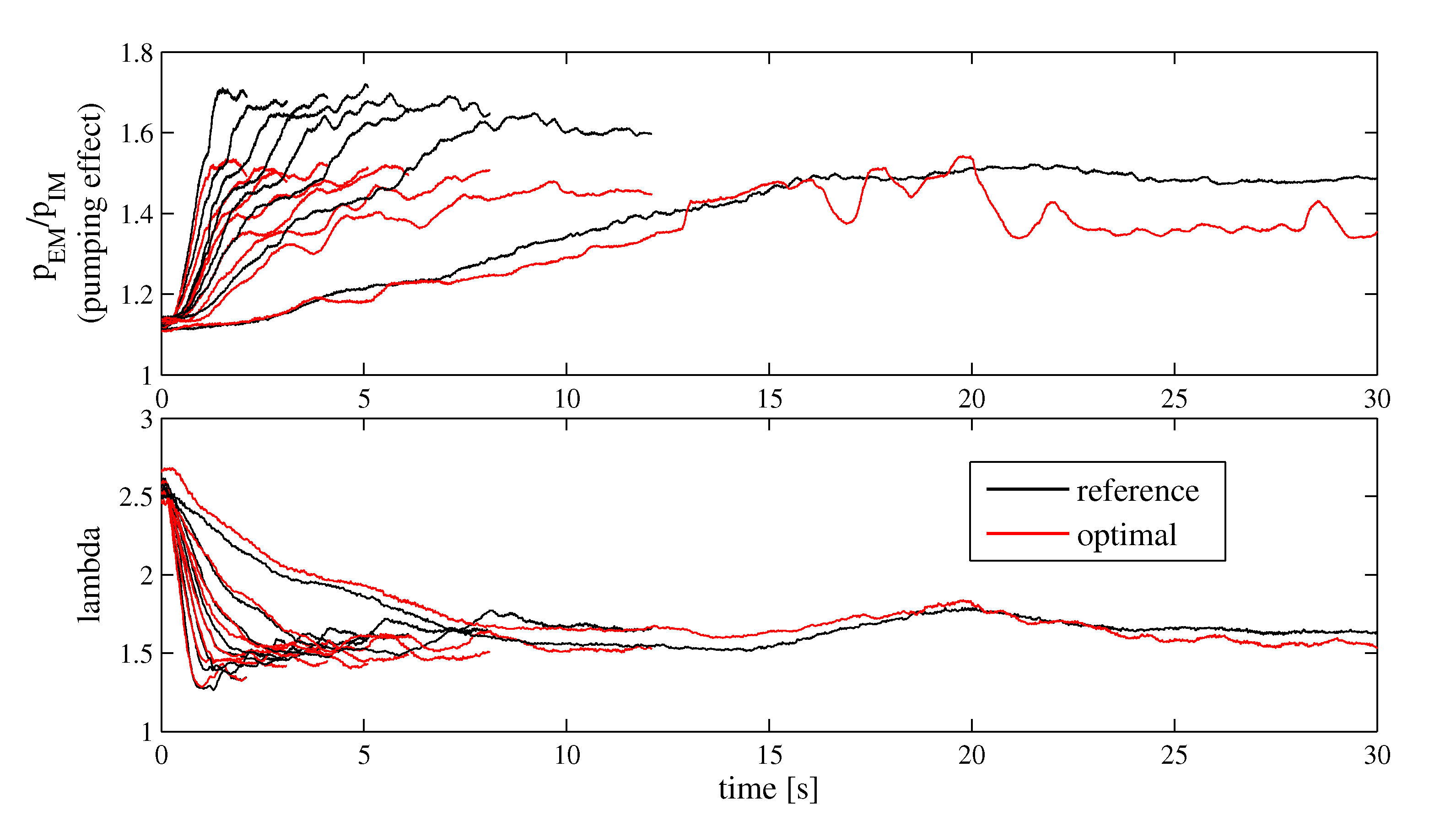Looking at Figure 2, the slowest ramp (30 s duration) can be considered to represent the static case, i.e., to consist of a sequence of steady-state conditions. The results in Table 2 show cumulative fuel consumption, NO_x and soot emissions variations with respect to this stationary-like profile. From now on, the values of the three quantities just mentioned are always normalized with respect to the integrated engine power, to allow for meaningful comparisons. It turns out that the higher is the load gradient, the higher is the specific fuel consumption. Despite this statement could be quite predictable, figuring out the responsible physical effect is of sure interest. The third graph in Figure 2a shows that the increasing pumping effect corresponding to increasing gradients, is the main reason for the fuel penalty. In other words, the faster is the transient the higher is the negative backpressure effect caused by the turbine. This effect disappears as soon as quasi-static state conditions are reached.

Figure 1. Feedforward (FF) control based on the steady-state actuator set-point maps.

Figure 1. Feedforward (FF) control based on the steady-state actuator set-point maps.

Figure 2. Ramp profiles performed at 1950 rpm.

Figure 2. Ramp profiles performed at 1950 rpm.

Table 2. Effect of increasing load gradients: fuel, NOx and soot related to the integrated engine power (normalized quantities).

Ramp duration (s)	30	12	8	6	5	4	3	2
$\frac{d}{dt}{m}_{\text{fcc}}(\frac{{\text{mm}}^{\text{3}}}{\text{s}})$	1	2.5	3.75	5	6	7.5	10	15
fuel	0% (ref)	2.77%	4.34%	4.42%	5.31%	5.79%	6.73%	8.30%
NOx	0% (ref)	21.44%	30.91%	41.46%	44.42%	51.58%	57.55%	65.48%
soot	0% (ref)	-15.37%	-15.53%	-18.81%	-19.24%	-10.42%	-3.79%	31.83%

Table 2. Effect of increasing load gradients: fuel, NOx and soot related to the integrated engine power (normalized quantities).

Ramp duration (s)	30	12	8	6	5	4	3	2
$\frac{d}{dt}{m}_{\text{fcc}}(\frac{{\text{mm}}^{\text{3}}}{\text{s}})$	1	2.5	3.75	5	6	7.5	10	15
fuel	0% (ref)	2.77%	4.34%	4.42%	5.31%	5.79%	6.73%	8.30%
NOx	0% (ref)	21.44%	30.91%	41.46%	44.42%	51.58%	57.55%	65.48%
soot	0% (ref)	-15.37%	-15.53%	-18.81%	-19.24%	-10.42%	-3.79%	31.83%

This is the crucial point: a stationary lookup map by nature is not able to account for dynamic effects, so it sets the actuator set-point to the value that will be appropriate when the transient is over. This yields, for instance, a VGT position that increases the engine backpressure with negative effect on efficiency. When the VGT is closed in order to increase the IM pressure (p_IM), the exhaust pressure (p_EM) increases too, but with a faster dynamic, resulting in a growing effect of the backpressure. This is proven by the third graph which shows the ratio between p_EM and p_IM. Moreover, it is also true that the air handling system has a slower dynamic than the fueling system, so an air reservoir is needed to prevent an excessive air-to-fuel ratio (AFR) reduction during a positive load gradient. The fourth graph in Figure 2a proves this statement, showing the drop of the lambda value, ever more accentuated as the load gradient increases. The phenomenon just explained does not depend only on the TC but also on the EGR rate, so that the combined effect of these two control levers has to be taken into account.

Obviously all the considerations presented so far have also an influence on exhaust emissions, as shown in Table 2. Concerning NO_x emissions, there is a combined effect of the reduced amount of air entering the cylinders and the delayed effect of the EGR, which together lead to a higher combustion temperature. The soot trend is not as monotone as the NO_x one, and the reason can be related to several aspects. First of all, the measurement device is not fast enough to capture the transient peaks, resulting in a potentially misleading cumulative value. We also remind the reader that we are measuring raw emissions, while the traditional use of the engine at hand sees a diesel particulate filter (DPF) installed on the exhaust line, resulting in a drastic reduction of tailpipe soot emissions. Moreover, this aspect does not represent a limitation regarding the validity of the presented results, since, as remarked later, soot emissions are considered as a qualitative quantity not to be widely exceeded. Another control lever which strongly effects fuel efficiency and NO_x emissions is the crank angle corresponding to the start of injection (SOI). This control input directly influences the combustion process and thus no dynamics are related to it directly. However, it may be used to compensate for the transient effects described above, which is also proposed in [16]. For this reason, the SOI is included in the dynamic optimization procedure proposed below.

Once the indisputable effect of transients has been remarked on, it comes out that finding the perfect combination of multiple cross-coupled control inputs is a difficult engineering problem, which cannot be solved with just a calibration-based approach. We propose a synergy between mathematical models representing the engine, optimal control theory, and specific dynamics-accounting experiments carried out on the real engine. Before describing the new control structures derived, all methods concerning engine models and optimal control are outlined in the next sections.

2.2. Engine Model

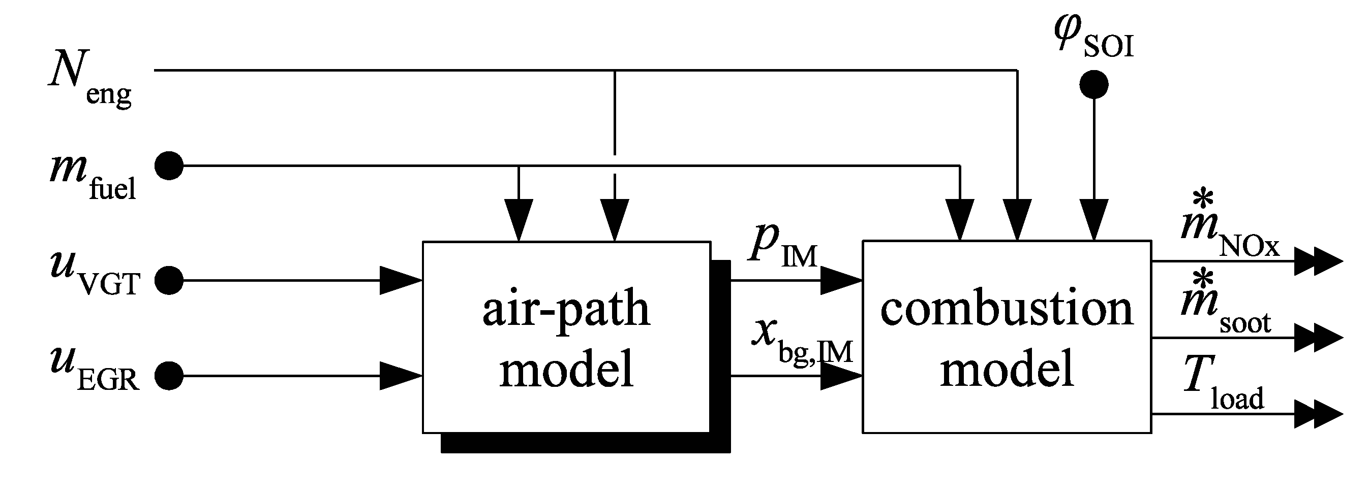
The model can be subdivided into a dynamic and a static part as illustrated in Figure 3. The subscripts denote the intake and exhaust manifolds (IM/EM), the volume between the turbine and the exhaust-gas aftertreatment system (ATS), and the TC. The positions of the VGT and the EGR valve are pulse-width modulation signals with a range of [0,1]. The SOI is specified in degrees before top dead center (BTDC). Finally, the burnt-gas fraction in the IM is denoted by x_bg,IM.

Figure 3. Structure of the engine model.

Figure 3. Structure of the engine model.

All dynamics are induced by the air path, i.e., the TC inertia and the volumes. The full model is represented in state-space form as:

$$\dot{x}(t)=f(x(t),u(t))$$

(1a)

$$y(t)=g(x(t),u(t))$$

(1b)

where the n_x = 6 state variables, the n_u = 3 control inputs, and the outputs are:

x = (p_IM, ϑ_IM, x_bg,IM, p_EM, p_aTB, ω_TC)^T

(2a)

$$u={(u_{\text{VGT}},u_{\text{EGR}},{\phi }_{\text{SOI}})}^T,y={({\stackrel{*}{m}}_{{\text{NO}}_x},{\stackrel{*}{m}}_{\text{soot}},T_{\text{load}})}^T$$

(2b)

The engine speed (N_eng) and the fuel mass injected (m_fcc) are treated as time-varying parameters, moreover both are fixed during the optimization procedure. The outputs of the air-path model, i.e., the dynamic inputs to the combustion model, are denoted by v := (p_IM, x_bg,IM)^T, with:

(3)

2.2.1. Air-Path Model

The mean-value model for the air path, adopted from [13], is extended to include the EGR, and an additional restriction representing the exhaust-gas ATS. The new model parts are briefly described next.

The EGR valve is modeled as a modified form of the simplified isenthalpic orifice [1] with a variable effective cross-sectional area:

(4)

For the temperature difference across the exhaust gas cooler (EGC), a simple stationary energy balance is evaluated. The average of the inflow and outflow temperatures is used as the representative temperature, which yields:

$$k_{\text{EGC}}\cdot \left(\frac{{\vartheta }_{\text{EM}}+{\vartheta }_{\text{EGR}}}{2}-{\vartheta }_{\text{clf}}\right)={\stackrel{*}{m}}_{\text{EGR}}·({\vartheta }_{\mathrm{EM}}-{\vartheta }_{\text{EGR}})$$

(5a)

The temperature of the cooling-fluid is assumed to be constant, i.e., ϑ_clf = 360 K, and the efficiency parameter kEGC depends on the mass flow:

$$k_{\text{EGC}}=k_{\text{EGC,1}}\cdot {\stackrel{*}{m}}_{\text{EGR}}+k_{\text{EGC,2}}\cdot {\stackrel{*}{m}}_{\text{EGR}}$$

(5b)

Differential equations: The change of the state variables, i.e., the equations defining Equation (1a), represent balances for mass and energy. In the intake receiver, the mass balances for the air and the burnt gas as well as the energy balance is resolved for the state variables pressure, temperature and burnt-gas fraction $x_{\text{bg,IM}}:=\frac{m_{\text{bg}}}{m_{\text{air}}+m_{\text{bg}}}$:

$$f_1=\frac{d}{dt}{p}_{\text{IM}}=\frac{R}{V_{\text{IM}}}\text{κ}\left({\stackrel{*}{m}}_{\text{CP}}{\vartheta }_{\text{IC}}+{\stackrel{*}{m}}_{\text{EGR}}{\vartheta }_{\text{EGC}}-{\stackrel{*}{m}}_{\text{cyl}}{\vartheta }_{\text{IM}}\right)$$

(6a)

$$f_2=\frac{d}{dt}{\vartheta }_{\text{IM}}=\frac{R{\vartheta }_{\text{IM}}}{p_{\text{IM}}{V}_{\text{IM}}{c}_v}\left[c_p\left({\stackrel{*}{m}}_{\text{CP}}{\vartheta }_{\text{IC}}+{\stackrel{*}{m}}_{\text{EGR}}{\vartheta }_{\text{EGC}}-{\stackrel{*}{m}}_{\text{cyl}}{\vartheta }_{\text{IM}}\right)–c_v{\vartheta }_{\text{IM}}\left({\stackrel{*}{m}}_{\text{CP}}+{\stackrel{*}{m}}_{\text{EGR}}-{\stackrel{*}{m}}_{\text{cyl}}\right)\right]$$

(6b)

$$f_3=\frac{d}{dt}{x}_{\text{bg,IM}}=\frac{R{\vartheta }_{\text{IM}}}{p_{\text{IM}}{V}_{\text{IM}}} \left({\stackrel{*}{m}}_{\text{EGR}}{x}_{\text{bg,EM}}-\left({\stackrel{*}{m}}_{\text{EGR}}+{\stackrel{*}{m}}_{\text{CP}}\right)\cdot x_{\text{bg,IM}}\right)$$

(6c)

The subscripts CP and IC denote quantities corresponding to the compressor and the charge-air intercooler, respectively. The burnt-gas fraction in the exhaust gas is:

$$x_{\text{bg,EM}}=\frac{x_{\text{bg,IM}}·{\stackrel{*}{m}}_{\text{cyl}}+(1+{\sigma }_0)·{\stackrel{*}{m}}_{\text{fuel}}}{{\stackrel{*}{m}}_{\text{cyl}}+{\stackrel{*}{m}}_{\text{fuel}}}$$

(7)

where σ₀ is the stoichiometric ratio of air and fuel flow (or mass) into the cylinder. A simple mass balance is applied in the volume between turbine and ATS, and a momentum balance defines the change of the TC speed, see e.g., [1,13].

2.2.2. Combustion Model

Time-variable quadratic setpoint-deviation models are used for the emissions and for the combustion efficiency. The vector w =(p_IM, x_bg, φ_SOI)^T denotes all inputs to the combustion model. The model for each output thus reads:

$$y_i(t)=y_{\text{ref},i}(t)+k_{\text{lin}}{(t)}^T\cdot \Delta w(t)+\Delta w{(t)}^T\cdot K_{\text{quad}}(t)\cdot \Delta w(t)$$

(8a)

with:

$$K_{\text{quad}}(t)=\text{diag}\left(k_{\text{quad,1}}(t),\mathrm{...},k_{\text{quad,3}}(t)\right)$$

(8b)

$$\Delta w(t)=w(t)-w_{\text{ref}}(t)$$

(8c)

As can be noticed, the input to the combustion model is not exactly the vector w, but rather its variation with respect to a reference vector. A detailed description of the identification procedure is presented in Section 2.6, however the reference condition is nothing other than the starting ramp profile, while the real input Δw is generated by performing several variations of the control inputs along the reference trajectory. Such setpoint-relative models are often used for control and optimization applications [17,18]. 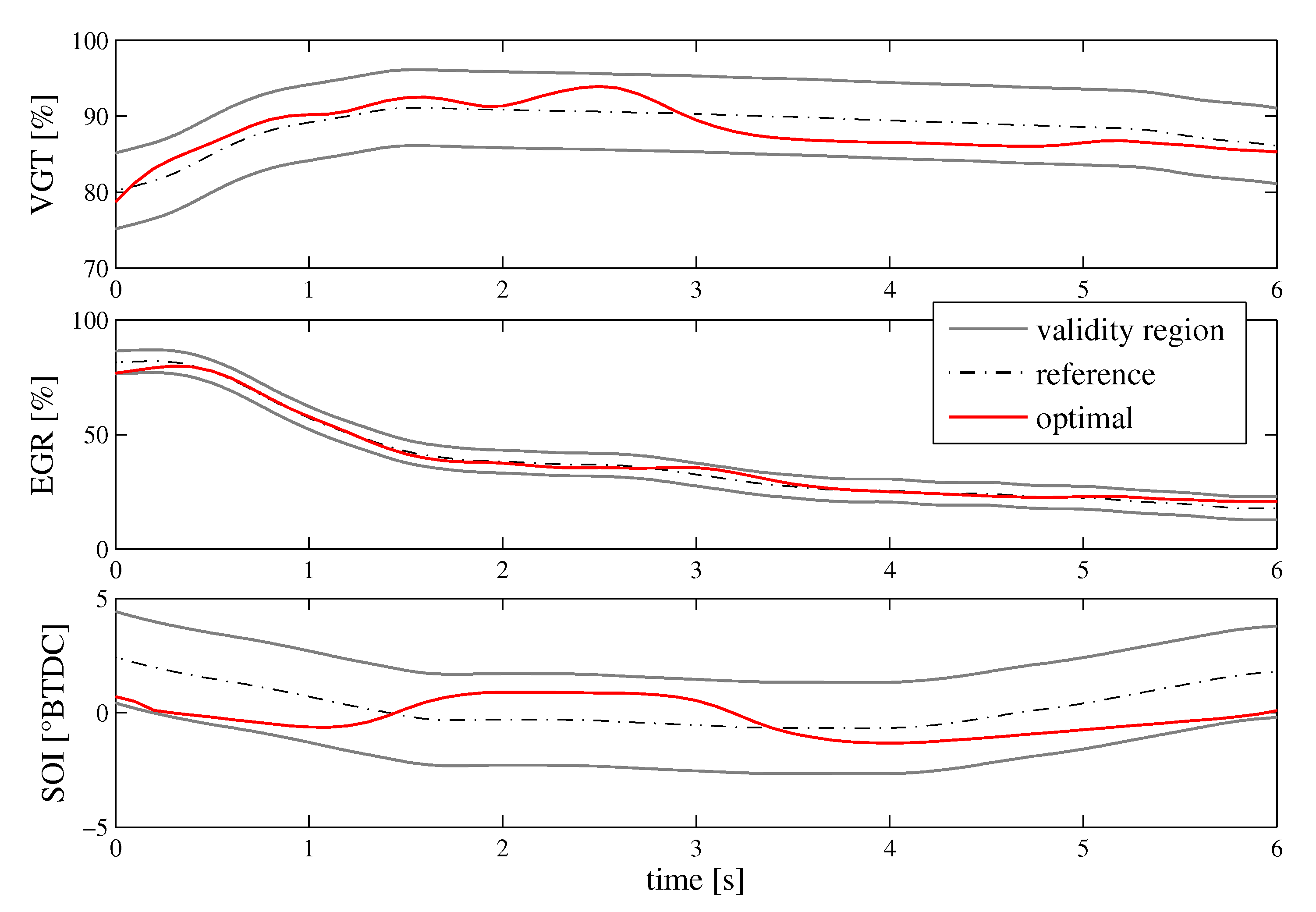The cross-terms of the full second-order Taylor expansion are omitted since also the n_u(n_u − 1)/2 cross variations would need to be performed to reliably identify the corresponding model coefficients. The effect of omitting the cross terms has been analyzed, resulting in a negligible effect on the combustion model accuracy. Usually the references for the inputs w are stored as static lookup maps over engine speed and load. During transient operation, such as the ramps shown in Figure 2, the actual values of the dynamic inputs (p_IM and x_bg,IM in the case at hand) can be far from the steady-state reference values. By using time-resolved reference values and correction factors, the validity range of the model is relocated to the actually relevant region, which is illustrated in Figure 4.

Figure 4. Exemplary static and dynamic references over a load step, and the validity regions of the corresponding setpoint-relative models.

Figure 4. Exemplary static and dynamic references over a load step, and the validity regions of the corresponding setpoint-relative models.

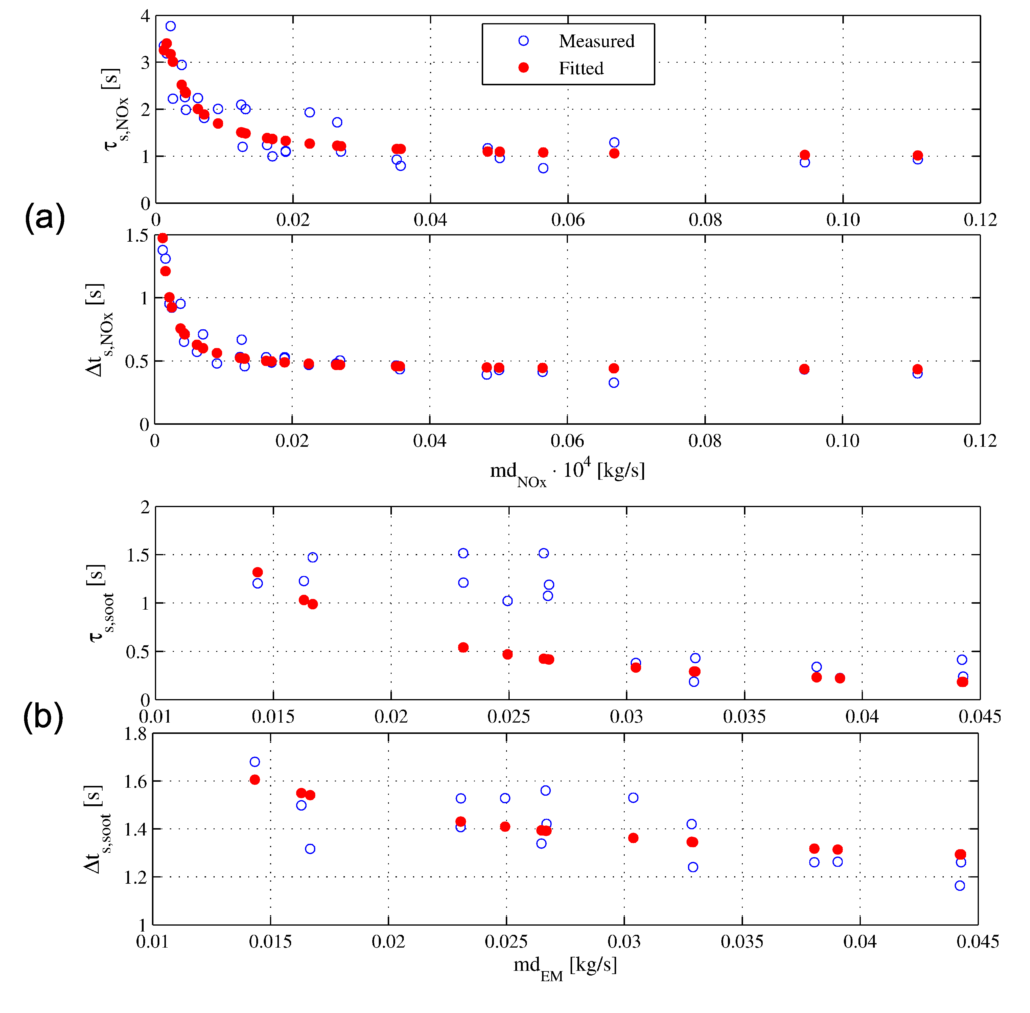
2.3. Sensor Dynamics of the NO_x and Soot Sensors

A further critical aspect regarding empirical modeling of engine-out emissions, is the phase shift between transient engine events and transient emission measurements. In the case at hand the NO_x emissions are measured by a Continental UniNO_x sensor, while the soot emissions are recorded by means of an AVL Micro Soot Sensor. Accounting for the transient transport delays and sensor lags, which together constitute the phase shift, is very important for the quality of the model prediction. For this reason, the dynamic characteristic of the sensor signals has been modeled as a first-order lag element, with a time delay resulting from the transport of the gas to the sensor. The signal ξ_s,i of emission sensors, can thus be expressed by the differential Equation (9), where i corresponds to the emission species NO_x or soot:

$$\frac{d}{dt}{\xi }_{s,i}(t)=-\frac{1}{{\tau }_{s,i}}\cdot \left[{\xi }_{s,i}(t)-{\text{ψ}}_i(t-\Delta t_{s,i})\right]$$

(9)

the variable ψ_i refers to the corresponding engine-out emission species that reaches the sensor after a delay of Δt_s,i. In order to influence the engine-out emissions separately, measurements with stepwise changes in the SOI and in the EGR valve have been carried out, for several engine speeds and loads. The recorded emission signals have then been used to identify the sensor dynamics of the NO_x and soot sensors, respectively. Figure 5 shows the results of the identification. Interesting correlations with the NO_x mass flow (md_NOx in figure) and the total exhaust mass flow (md_EM in figure) have been observed, respectively for the NO_x and soot sensors. For this reason, the fitted curves shown in red dots have been used to account for the sensors dynamics within the combustion model. Note that the dynamic characteristics of the Micro Soot Sensor are significantly influenced by the dilution ratio. In the event of low ambient temperatures or insufficiently diluted exhaust gas there is the risk of the formation of condensate in the measuring chamber. In order to avoid condensate formation, sufficient dilution of the exhaust gas should be provided for. On the other hand, the delay and the time constant are smaller for low dilution ratios. As a compromise a dilution ratio of 5 (in a range of 2–20) has been used for the experiments.

Figure 5. Trend of the time constant τ_s,i and the time delay Δt_s,i identified for: (a) NO_x sensor; and (b) soot sensor.

Figure 5. Trend of the time constant τ_s,i and the time delay Δt_s,i identified for: (a) NO_x sensor; and (b) soot sensor.

2.4. Numerical Optimal Control

The optimal control problem (OCP) considered here can be cast in the following form:

$$\underset{u(·),x(·)}{\text{max}}\{E_{\text{load}}={\displaystyle {\int }_0^{t_f}{T}_{\text{load}}}(x(t),u(t),m_{\text{fcc}}(t))\cdot N_{\text{eng}}dt\}$$

(10a)

$$\text{s.t. }\dot{x}(t)-f(x(t),u(t),m_{\text{fcc}}(t),N_{\text{eng}})=0$$

(10b)

$${\displaystyle {\int }_0^{t_f}{\stackrel{*}{m}}_{\text{em}}(x(t),u(t),m_{\text{fcc}}(t),N_{\text{eng}})dt}-{\widehat{m}}_{\text{em}}\le 0$$

(10c)

$$\underset{\_}{u}(t)\le u(t)\le \overline{u}(t),\underset{\_}{x}(t)\le x(t)\le \overline{x}(t)$$

(10d)

With $m_{\text{em}}={(m_{{\text{NO}}_x},m_{\text{soot}})}^T$.

The cost function is the integrated power over the load ramp profile, called E_load in Equation (10a). The instantaneous fuel mass flow ${\stackrel{*}{m}}_{\text{fuel}}=m_{\text{fcc}}\cdot \frac{N_{\text{eng}}}{120}\cdot N_{\text{cyl}}$ is integrated to yield the cumulative fuel consumption m_fuel. The true objective would be the minimization of the specific fuel consumption, which can be expressed as: $=\frac{m_{\text{fuel}}}{E_{\text{load}}}\left(\frac{\text{g}}{\text{kW}\cdot \text{h}}\right)$, but the fuel quantity is assigned for each ramp, so it never changes. Consequently, the target becomes the maximization of the energy released, in other words the net engine power (or T_load being N_eng constant). The dynamic constraints in Equation (10b) enforce the model equations and Equation (10c) limits the cumulative emissions. Considering that the soot measurements exhibit a large variability, which is also present in the identification data, the corresponding model is not as reliable as the NO_x model. Despite that, a cumulative constraint for soot emissions is anyways set during the optimization, but more permissive, otherwise the optimization could be negatively effected, resulting in a suboptimal solution for the main objective. Detailed information about the numerical methods required for optimal control of diesel engines may be found in [14].

Direct transcription. The continuous-time OCP in Equation (10) is transformed into a finite-dimensional mathematical program by direct transcription. The Euler-backward integration scheme is applied to consistently discretize the full problem. The set of differential Equation (10b) is transformed to:

x_k+1 = x_k + h · f(u_k+1, x_k+1, m_fcc,k+1, N_eng,k+1)

(11)

where x_k:= x(t_k). A uniform step size of h = 0.1s is used. All integrals are approximated as a sum:

(12)

where N denotes the total number of discretization points. The bounds on the control inputs and on the state variables are imposed at the discretization points. The resulting mathematical program has the values of the control inputs and the state variables at the discretization points as decision variables. It can be solved efficiently due to its sparse structure [19]. In this work, the solver Sparse Nonlinear OPTimizer (SNOPT) is used [20].

2.5. Experimental Setup

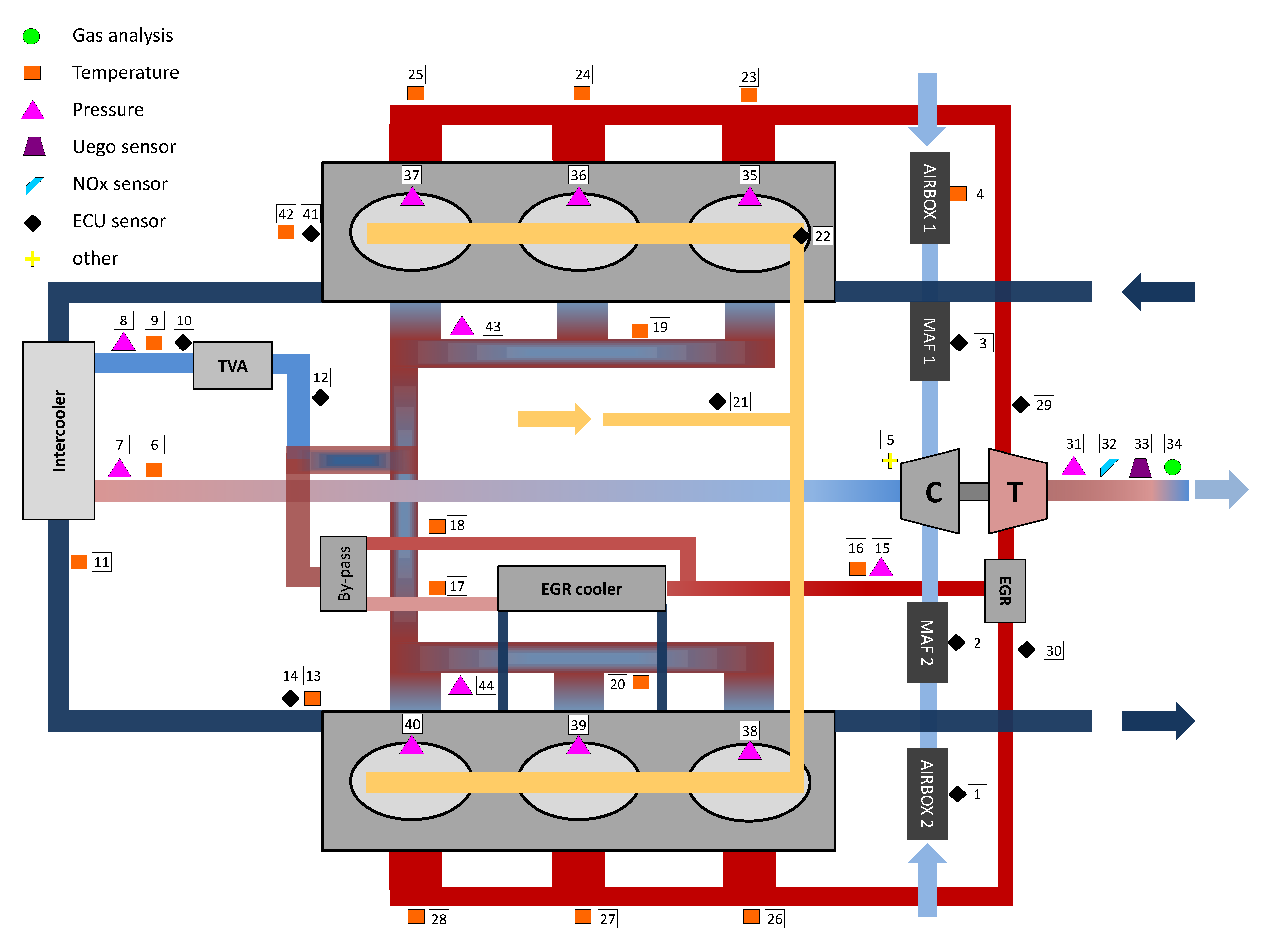
All measurements are performed on the diesel engine specified in Table 1. The signals required to identify the air-path model are obtained from standard electronic control unit (ECU) sensors installed on the engine as well as some additional sensors for the temperature and the pressure at specific locations. Figure 6 shows the sensors’ layout installed on the diesel engine used in this work. The testbench is equipped with a dynamic brake which is controlled by a dSPACE rapid prototyping system. This system is able to prescribe arbitrary profiles for the engine speed and load.

Figure 6. Layout of the diesel engine used in this work, showing the various types of sensors installed. ECU: electronic control unit.

Figure 6. Layout of the diesel engine used in this work, showing the various types of sensors installed. ECU: electronic control unit.

The engine is controlled by a development ECU, which slightly differs from the end of line version implemented on the production vehicle. The Ethernet-based ETK interface by ETAS (Stuttgart, Germany) provides direct access to the control variables and parameters of the ECU via the parallel data and address bus, or via a serial microcontroller testing or debugging interface. The ETK interface is real-time capable, and provides a universal ECU interface for sophisticated applications in the development and calibration of engine ECUs. The interface is supported across the board by ETAS hardware modules, the INCA calibration tool as well as the INTECRIO and ASCET development tools. The need to develop, add and/or bypass some control structures implemented on the ECU has been fulfilled by the utilization of a Rapid Prototyping Module (ES910 by ETAS), in combination with the software package INCA-experimental target integration package (EIP). INCA-EIP enables real-time function developers to use the measurement and calibration functionality of INCA while the ECU software functions are executed on the ES910. The ES910 prototyping and interface module combines high computing performance with all common ECU interfaces in a compact and robust housing. A schematic representation of its interaction with the ECU and the Host PC is shown in Figure 7. CAN and LIN interfaces provide the connection of the ES910 module to the ECU bus and to the external CAN-modules (input/output operations). This setup provides complete control over all relevant control inputs of the engine.

Figure 7. Hardware, software, and interfaces of the testbench setup. EIP: experimental target integration package.

Figure 7. Hardware, software, and interfaces of the testbench setup. EIP: experimental target integration package.

The prototyping tool INTECRIO is used to set up the rapid-prototyping models, previously designed in Simulink (by MathWorks, Natick, MA, USA) on the ES910. During the INTECRIO experiment the user has runtime access to the model executed by the ES910 module. With such an experimental setup any ECU function can be bypassed, allowing for the development and the implementation of custom control algorithms. In the case at hand, the by-pass functionalities needed to perform the ramp profiles have been developed in Simulink by designing a custom engine management software for this exact purpose. Each control input profile, corresponding to the requested ramp, is set up and uploaded before running the test; when the stationary condition is reached, the by-pass is activated and the ramp is performed.

2.6. Optimization Procedure

The dynamic optimization procedure relies on two modes of operating the engine:

• The ECU with its standard calibration controls the engine, in particular it prescribes the fuel profile related to each ramp. The testbench controller has to guarantee the desired engine speed (constant in this case). This mode is used for the initialization of the optimization procedure. The resulting trajectories of the controls (VGT, EGR and SOI) are recorded.
• Time-resolved trajectories are prescribed for all control inputs using the rapid-prototyping module and the bypasses of the ECU. The testbench controller has exactly the same task as in Mode A). This mode is used for all variations runs as well as for validation.

The inputs to the procedure are the transient profiles of Figure 2, performed one at a time, by using a standard engine calibration that is able to operate the engine along this profile. The following list describes the individual steps of the dynamic optimization:

• Initialization: drive the profile in Mode A. Save the resulting trajectories of the control inputs u(t).
• Perform 1 + 4·n_u testbench runs in Mode B. Thereby, apply:

  (a)

  the reference controls u(t), and

  (b)

  two perturbations of all controls towards each direction, i.e.,

  u_i(t) ← u_i(t) ± {0.5·Δu_i, Δu_i}, for i = 1, ..., n_u.

  Run simulations of the air-path model for all variations.
• Use the state trajectories of the air-path model and the measured emission and torque trajectories from Step 2, to identify the torque and emission models around the current references.
• Solve the control and state constrained OCP in Equation (10) to derive the improved control trajectories u^∗(t). Thereby, set:

  u(t) = u(t) − Δu,   u(t) = u(t) + Δu

  (13)

Using the simulated state trajectories during the identification of the combustion model in Step 3 ensures a consistent prediction of the emissions and of the torque inside the validity region. Since the identification of the models for the air path and for the combustion are identified separately, the physical causality is preserved. More exactly, there is no way that the combustion model corrects errors in the air-path model or vice-versa. Although a combined identification could yield a slightly higher accuracy, it would introduce unphysical cross corrections. Furthermore, the identification procedure would become more complex and non-convex.

In order to automate the optimization procedure, it has been necessary to manage remotely some basic functionalities provided by INCA, such as setting calibrations, reading signals and recording measurements. This additional functionality can be achieved through several methods; our choice consisted in a COM communication established between Matlab and INCA, by means of an in-house Matlab script.

2.7. From Time-Based to Map-Based Optimal Control

The optimal control input set, achieved with the optimization procedure, is non causal and valid only for the specific profile used for the optimization, as opposed to a conventional table or map-based control structure. Moreover, if we refer to Figure 1, there is not a unique optimal trajectory for a given speed, but several, corresponding to each ramp performed. It is thus of particular interest to find a way to transform these control trajectories to an operating point based representation, while preserving the information about the optimal solution. Accepting the fact that it is unfeasible to keep intact the content of the time-resolved control vector, its information could be stored in a scalar value of a new lookup table, namely the transient compensation map. Since this map has to be activated only when transients occur, a direct dependency with the load gradient is needed. Therefore, the second quantity, besides the engine speed, that spans the compensation maps is the derivative of the fuel quantity, while the fuel quantity itself is used for the steady-state maps.

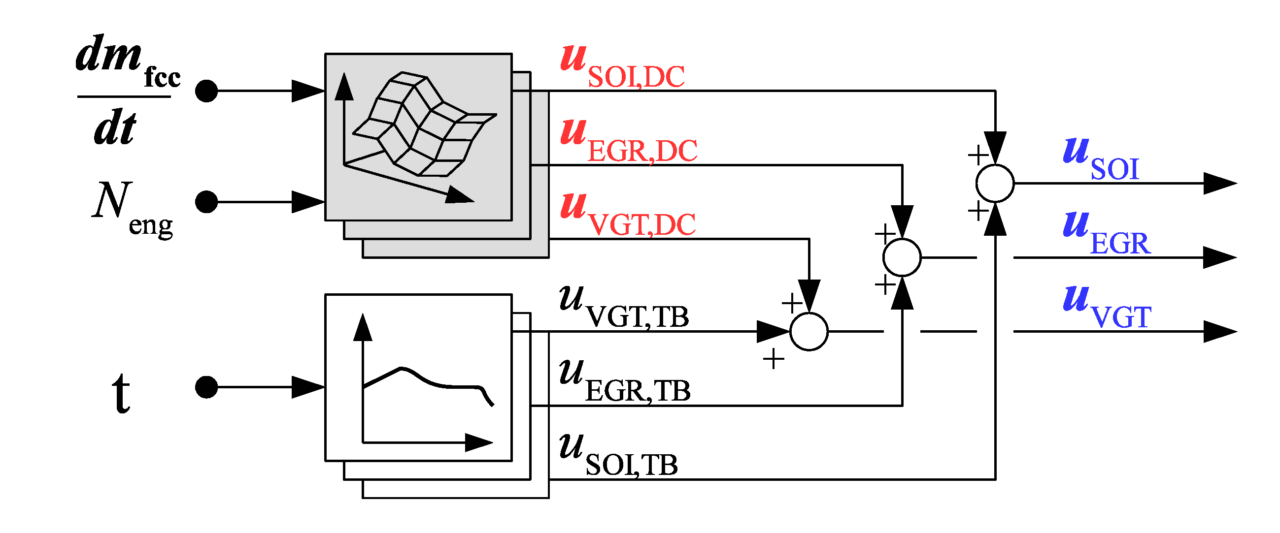
Figure 8 shows the two solutions proposed, both based on compensation maps that contain the information derived from the solution of the OCP. What distinguishes the two control structures is the way the cylinder charge is managed, while the SOI is treated identically. Controlling the cylinder charge is equivalent to controlling the IM pressure pIM and the burnt-gas fraction x_bg,IM, by means of EGR and VGT, which represent the relevant actuators. In the first case, as shown in Figure 8a, the physical conditions in the IM are not considered at all, resulting in a FF control based on the steady-state actuator set-point maps. Because of its simplicity, this control structure is still used as basic layer in engine control systems. Unfortunately, as soon as a transient occurs all its limits come to light, suggesting that a pure steady-state approach is not satisfactory anymore. Enhancing its performance, by adding information related to transient operation, can be an interesting solution, especially if such a simple structure can be preserved. The compensation maps are highlighted, and their outputs are the dynamic compensation (DC) factors to be applied to VGT and EGR. If the load request gradient is below a certain threshold, set within the compensation map, there is no alteration of the stationary actuator set-point.

Figure 8. (a) FF control based on the steady-state actuator set-point maps: compensation of actuator set-point values; and (b) feedback (FB) control of the state variable set-point maps: compensation of state variable set-point values.

Figure 8. (a) FF control based on the steady-state actuator set-point maps: compensation of actuator set-point values; and (b) feedback (FB) control of the state variable set-point maps: compensation of state variable set-point values.

The second case, shown in Figure 8b, is characterized by an alternative and more complex kind of cylinder charge control, called air-path control. In this case, the actuation of VGT and EGR are feedback (FB) controlled, therefore the set-point variables are p_IM and x_bg,IM. The implementation of this advanced control structure has been possible thanks to the rapid control prototype (RCP) system presented in Section 2.5. All details about the air-path controller implemented and used during the experimental validation, can be found in [21]. Differently from the previous case, the lookup tables store the steady-state set-points of the two state variables mentioned above. At the same time, the compensation maps act directly on these references for the FB controller. If the correction was applied directly to the actuators (u_VGT,FB and u_EGR,FB), it would act as a disturbance that the FB controller would try to compensate.

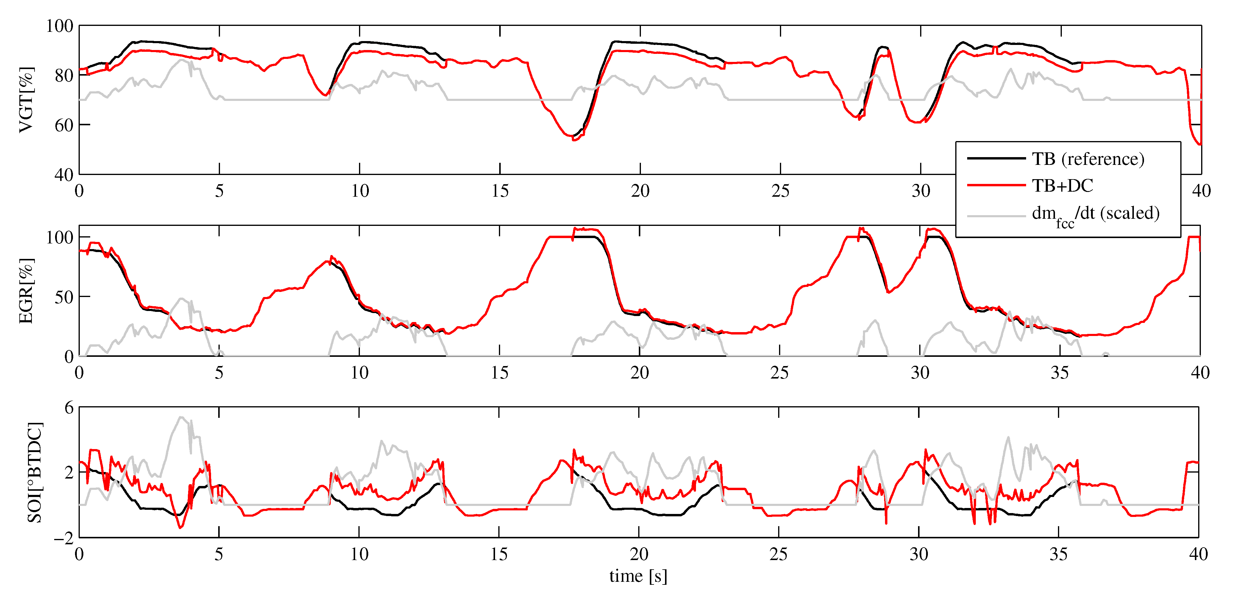
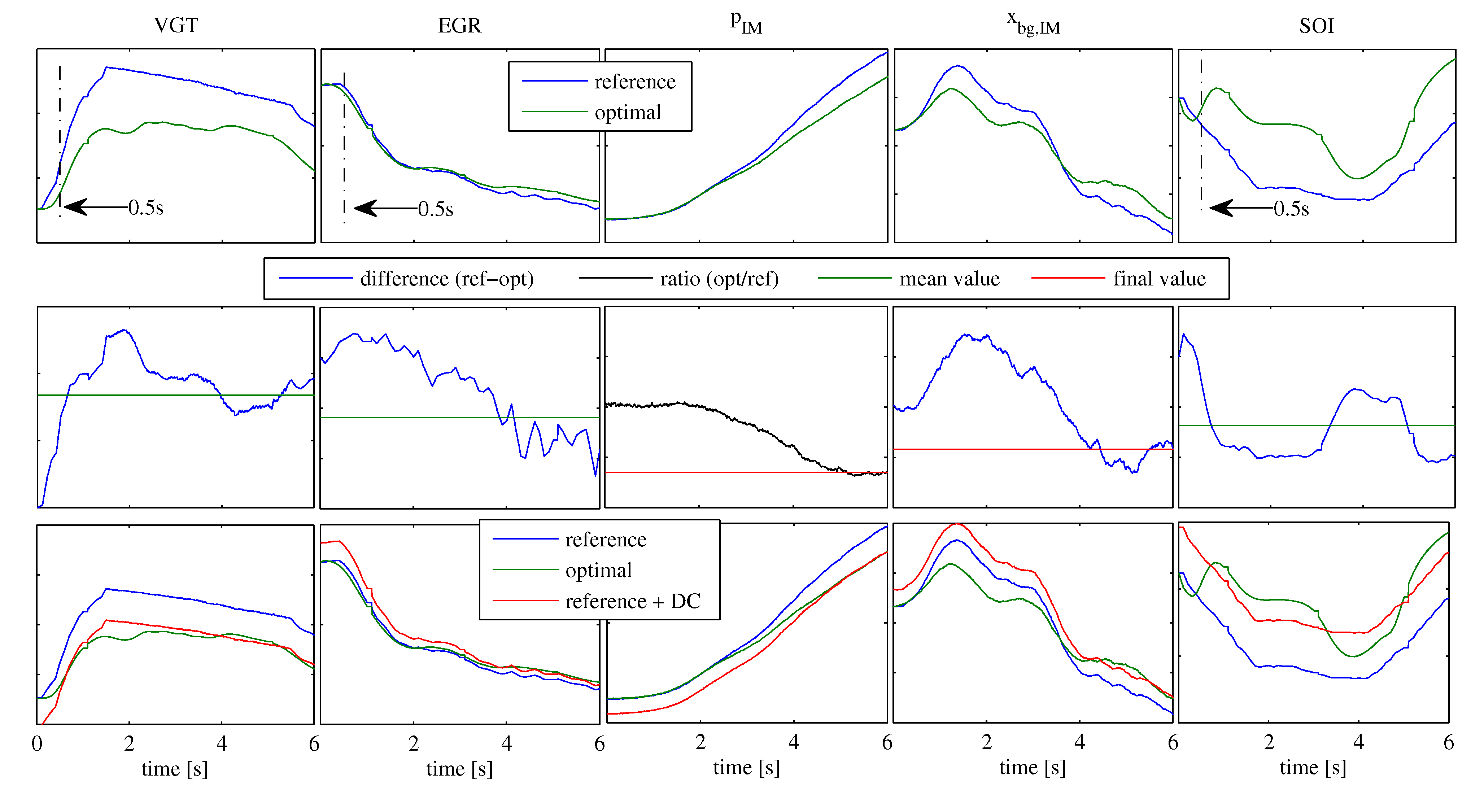
Regardless of the control structure, the DC maps have the goal to reproduce as strictly as possible the optimal trajectories. Figure 9 helps explaining how they have been derived, for one exemplary ramp profile. In the first row is shown the comparison between the reference trajectory, obtained by using a standard engine calibration with the ECU running in Mode A, and the optimized trajectory (Section 2.6). VGT and EGR profiles are the real optimal control inputs derived from the optimization procedure, while p_IM and x_bg,IM profiles are the corresponding measurements. Since we are considering one single ramp profile, which means a single value of the fuel derivative, a single scalar value has to capture the information coming out from this comparison. The second row shows how the scalar value is calculated. For VGT and EGR, it is the mean value of the difference between optimal and reference trajectory, starting 0.5 s after the actual ramp starts (dash-dot line), since the initial conditions of reference and optimal controls coincide. For p_IM and x_bg,IM, the final value of, respectively the ratio and the difference between the trajectories is considered. The third and final row highlights the differences between optimal solutions and dynamically compensated reference control inputs. Coherently with the distinction made between the two control structures, VGT and EGR refer to Case (a) while p_IM and x_bg,IM refer to Case (b). For what concerns the SOI, its compensation is identical, no matter the control structure, and likewise to the VGT and EGR cases, the average difference is used to calculate the correction factor (last column).

Figure 9. Example of calculation of the dynamic compensation (DC) factor, for the 6 s ramp. First row: comparison between reference and optimal trajectories. Second row: difference (blue line) and ratio (black line) between optimal and reference trajectories. Compensation factors are derived by using either the average (green line) or the final value (red line) of the respective compensation vectors. Third row: comparison between optimal solutions and dynamically compensated reference control inputs.

Figure 9. Example of calculation of the dynamic compensation (DC) factor, for the 6 s ramp. First row: comparison between reference and optimal trajectories. Second row: difference (blue line) and ratio (black line) between optimal and reference trajectories. Compensation factors are derived by using either the average (green line) or the final value (red line) of the respective compensation vectors. Third row: comparison between optimal solutions and dynamically compensated reference control inputs.

3. Results and Discussion

Firstly, the results obtained from the dynamic optimization are presented, by focusing on the capabilities of the optimization tool. Afterwards, it is presented a validation that has the aim of assessing the potential of this novel approach to dynamic FF control. Since the goal was to stimulate the dynamic response of the engine, a transient demanding cycle has been employed.

3.1. Dynamic Optimization

The outputs resulting from the solution of the OCP laid inside the validity region in Equation (10d) without being constrained. This fact implies that the variations of the inputs chosen, namely Δu_VGT = 0.05, Δu_EGR = 0.05 and Δu_SOI = 2, yield a good compromise between model quality and broadness of the validity region. If such outputs were limited by the validity limits, a second dynamic optimization would be necessary, shifting the validity region in order to leave the optimiser work properly.

Figure 10 shows an exemplary solution coming out from the optimization framework.

Figure 10. Optimal control-input trajectories for 6 s duration ramp.

Figure 10. Optimal control-input trajectories for 6 s duration ramp.

Table 3 shows the relative changes between the optimal and the reference time-based (TB) control input set, in terms of fuel consumption and emissions, related to the total energy released.

Table 3. Results of the dynamic optimization for each ramp. Relative changes between optimal and reference condition (average value over five repetitions).

Ramp duration (s)	2	3	4	5	6	8	12	30
Fuel, measured	−2.81%	−4.58%	−3.93%	−4.58%	−3.91%	−4.50%	−3.79%	−0.6%
NOx, measured	3.96%	10.4%	−1.53%	−3.85%	−12.92%	−15.87%	−14.73%	−0.49%
Soot, measured	−40.84%	−28.66%	−13.58%	−5.63%	0.75%	−0.92%	−4.09%	−30.70%

Table 3. Results of the dynamic optimization for each ramp. Relative changes between optimal and reference condition (average value over five repetitions).

Ramp duration (s)	2	3	4	5	6	8	12	30
Fuel, measured	−2.81%	−4.58%	−3.93%	−4.58%	−3.91%	−4.50%	−3.79%	−0.6%
NOx, measured	3.96%	10.4%	−1.53%	−3.85%	−12.92%	−15.87%	−14.73%	−0.49%
Soot, measured	−40.84%	−28.66%	−13.58%	−5.63%	0.75%	−0.92%	−4.09%	−30.70%

In addition, Figure 11 assesses the repeatability of the measurements, performed five times for each ramp, both for reference and for optimal conditions. The objective was to minimise fuel consumption, without penalizing NOx emissions in Equation (10c) and keeping soot emissions below an acceptable level. Regarding the former, a significant improvement of fuel efficiency has been accomplished, except for the slowest ramp (30 s duration). The result is plausible since that ramp is sufficiently slow to represent stationary operation. This result is also consistent with the assertion made in Section 2.1, where this ramp has been taken as the reference condition, in order to assess the effect of transient operation on fuel consumption.

Figure 11. Relative change of fuel consumption, NOx and soot emissions after the optimization. Average value and error bars calculated by repeating the measurement five time for each ramp.

Figure 11. Relative change of fuel consumption, NOx and soot emissions after the optimization. Average value and error bars calculated by repeating the measurement five time for each ramp.

Another proof of the effectiveness of the optimization is the reduction of the pumping effect as compared to suboptimal control of VGT and EGR performed by the production ECU. Figure 12 shows a comparison between the reference and the optimal solutions. The negative backpressure effect has been reduced, consistently with the observed fuel consumption reduction, without having compromised the AFR. Likewise to EGR and VGT, the SOI plays a fundamental role, due to its strong effect on fuel efficiency and NO_x emissions.

The usefulness of the optimization framework can be evaluated also from an other perspective. For example, we can suppose that the controller is asked to fulfill higher or lower NO_x emissions. In the first case, for instance, an even lower fuel consumption can be achieved, while accepting the increase of NO_x emissions (that could afterwards be reduced by means of an after-treatment system). This result can be obtained only if the engine model correctly predicts the NO_x-fuel tradeoff, and the optimization tool is able to cope with changing constraints. In order to assess this ability, NO_x constraint targets have been altered in positive or negative direction, for three cases representing fast, medium and very slow ramps.

The results are listed in Table 4, and demonstrate that the optimization framework is sensitive to the different requests of NO_x target, showing that lower NO_x emissions allow for higher improvement of fuel efficiency, and vice versa.

Figure 12. Comparison of the pumping effect and the air-to-fuel ratio (AFR) between reference and optimal ramp profiles.

Figure 12. Comparison of the pumping effect and the air-to-fuel ratio (AFR) between reference and optimal ramp profiles.

Table 4. Sensitivity analysis of the optimization framework, analyzed for three cases representing fast, medium and very slow ramps. Arrows indicate the NO_x target in qualitative form.

Ramp	NO x target	NO x measured	Fuel measured
5 s	↓	−16.86%	0.15%
30 s	↑	10.37%	−0.57%

Table 4. Sensitivity analysis of the optimization framework, analyzed for three cases representing fast, medium and very slow ramps. Arrows indicate the NO_x target in qualitative form.

Ramp	NO x target	NO x measured	Fuel measured
5 s	↓	−16.86%	0.15%
30 s	↑	10.37%	−0.57%

3.2. Optimal Control versus Compensation Maps

As explained in Section 2.7, the TB optimal control trajectories have to be transformed into a causal form, in order to be used for online control. Moreover, a simple map-based structure is chosen so that the transient compensation strategy may be directly implemented in a standard production ECU (Figure 8a).

Since the impossibility to exactly copy out the optimal trajectories, an analysis of the effects when going from the non-causal to the causal and implementable structure has been conducted.

To perform this analysis, a specific control structure has been used. It is shown in Figure 13. The ramp is performed and the air-path controller runs on the ECU, without any transient compensation. The control signals are recorded and then set as reference trajectories for the validation run. These control signals are referred as TB, and they can be applied only when using the ECU in B Mode. The DC maps act directly on the reference trajectories. This case, from now on called (TB + DC), is not implementable outside dedicated testbench setup, but it is the closest one to the optimal TB control. Therefore, this procedure allows assessing the effects of switching from the non-causal optimal solution to the map-based representation isolated from other influences.

Figure 13. Time-based (TB) control of actuator set-points: compensation of the time-resolved reference values.

Figure 13. Time-based (TB) control of actuator set-points: compensation of the time-resolved reference values.

Table 5 displays the relative changes with respect to the reference trajectories. As expected, a deterioration of the fuel efficiency is unavoidable, but the positive effect produced by the DC is still recognizable.

Table 5. Effect of the implementation of the compensation maps, for three cases representing very fast, fast and medium ramps. Comparison to optimal TB control, in terms of relative change with respect to reference trajectories.

Ramp duration (s)	Fuel	NOx	Soot
2, optimal	−2.81%	3.96%	−40.84%
Ref + compens	−0.68%	−8.39%	31.67%
5, optimal	−4.58%	−3.85%	−5.63%
Ref + compens	−2.92%	4.33%	26.63%
8, optimal	−4.5%	−15.87%	−0.92%
Ref + compens	−3.00%	−1.89%	16.86%

Table 5. Effect of the implementation of the compensation maps, for three cases representing very fast, fast and medium ramps. Comparison to optimal TB control, in terms of relative change with respect to reference trajectories.

Ramp duration (s)	Fuel	NOx	Soot
2, optimal	−2.81%	3.96%	−40.84%
Ref + compens	−0.68%	−8.39%	31.67%
5, optimal	−4.58%	−3.85%	−5.63%
Ref + compens	−2.92%	4.33%	26.63%
8, optimal	−4.5%	−15.87%	−0.92%
Ref + compens	−3.00%	−1.89%	16.86%

3.3. Validation

The validation cycle is shown in Figure 14. It is important to remind the reader that all the methodology described has been applied for one engine speed (1950 rpm), therefore that speed has been used also for the validation cycle. Three cases, corresponding respectively to three different control structures, have been compared:

• TB + DC. The non-implementable solution presented in Section 3.2 (Figure 13).
• FF + DC. The FF control based on the steady-state actuator set-point maps runs on the ECU (Figure 8a). This is the easiest implementation possible, the compensation maps act on the FF actuator outputs.
• FB + DC. The air-path control introduced in Figure 8b runs on the ECU. Only the reference values for the air-path controller are changed, except for the SOI, which is the same as in Case 2. Although this implementation is as straightforward as the previous case, the basic control structure to which the compensation maps are added is more complex.

Figure 14. Validation cycle at constant engine speed of 1950 rpm. V_fcc is the volume of fuel injected per cycle per cylinder.

Figure 14. Validation cycle at constant engine speed of 1950 rpm. V_fcc is the volume of fuel injected per cycle per cylinder.

In order to analyze the effect of the transient compensation in more detail, we consider two different types of result. Beside the overall effect of the DC, we can account just for the sub-part of the cycle where the compensation is active, i.e., where the fuel derivative is non negative (Figure 15).

Figure 15. Control signals for Case 1. In order to highlight when the compensation occurs, the fuel derivative trend is superimposed on the graph.

Figure 15. Control signals for Case 1. In order to highlight when the compensation occurs, the fuel derivative trend is superimposed on the graph.

Both results for the three cases are summarized in Table 6. It turns out that the best result is achieved by implementing the Case 1, as we could expect. It serves as a benchmark or as a guideline to design alternative near-optimal control structures. The Case 3 is very promising, especially considering the fact that it can be applied easily, once an air-path control is available. The Case 2 falls slightly short of our expectations, because even if there is a significant fuel reduction, it substantially increases the NO_x emissions. Most likely NO_x emissions might be reduced to the detriment of fuel efficiency, according to the well known trade-off between these two quantities.

Table 6. Performance of the compensation-map based control systems on the validation cycle, in terms of relative change with respect to reference trajectories.

Implementation case		(1) TB + DC	(2) FF + DC	(3) FB + DC
Fuel	Overall	−2.08%	−1.68%	−1.22%
	Sub-part	−2.62%	−2.00%	−1.68%
NOx	Overall	0.28%	17.11%	−4.96%
	Sub-part	−0.19%	15.07%	−1.65%
Soot	Overall	−0.67%	−30.37%	18.05%
	Sub-part	−0.55%	−36.80%	25.96%

Table 6. Performance of the compensation-map based control systems on the validation cycle, in terms of relative change with respect to reference trajectories.

Implementation case		(1) TB + DC	(2) FF + DC	(3) FB + DC
Fuel	Overall	−2.08%	−1.68%	−1.22%
	Sub-part	−2.62%	−2.00%	−1.68%
NOx	Overall	0.28%	17.11%	−4.96%
	Sub-part	−0.19%	15.07%	−1.65%
Soot	Overall	−0.67%	−30.37%	18.05%
	Sub-part	−0.55%	−36.80%	25.96%

However, these results can be further explained by comparing the different control trajectories, as shown in Figure 16. It turns out that the higher the deviation of the control signals from the “optimal” solution (TB + DC), the worse the result. In fact, there is a discrepancy between the three cases in terms of the approximation of the optimal trajectories, especially for the EGR valve position within Case 2. Regarding the latter, the control inputs generated by using the ECU maps are rather far away from the optimal solution, and the transient maps cannot fully compensate such a deviation, resulting in a suboptimal result. However, the simplest Case 2, as opposed to the near-optimal but not implementable Case 3 which serves as a benchmark, has been employed to assess the effectiveness of the overall methodology.

Figure 16. Comparison between the three cases tested.

Figure 16. Comparison between the three cases tested.

4. Conclusions

A methodology to derive compensation maps suitable for the transient control of a diesel engine has been presented and experimentally validated. These maps are obtained by means of a dynamic optimization process, of which a beginning-to-end implementation and validation has been detailed. A significant improvement in terms of fuel efficiency, without compromising emission levels, can be achieved by applying the methodology presented. Moreover, the optimization framework shows a good sensitivity to the NO_x-fuel tradeoff when changing the NO_x emission constraints. As a consequence, the optimization tool can provide different levels of fuel reduction correspondingly to different tunings of the emission level targets.

Since the main goal was to test the overall validity of the methodology, only a single engine speed has been used. In order to cover the full operating range, the same procedure has to be repeated for different engine speeds. Thanks to the automated optimization procedure developed, the total time needed to perform a full calibration of the transient maps is directly proportional to the number of engine speeds spanned.

As concluded in Section 3.3, the transient maps cannot fully recover large deviations, typical of static control inputs significantly far away from the optimal solution. Therefore, further development of the methodology will focus on different approaches to extend the performance of the compensation maps to that case. An improvement could be achieved by deriving multi-dimensional maps which are able to reproduce more accurately the optimal solution.