Crude Oil Spot Price Forecasting Based on Multiple Crude Oil Markets and Timeframes

Abstract
: This study proposes a multiple kernel learning (MKL)-based regression model for crude oil spot price forecasting and trading. We used a well-known trend-following technical analysis indicator, the moving average convergence and divergence (MACD) indicator, for extracting features from original spot prices. Additionally, we factored in the possibility that movements of target crude oil prices may be related to other important crude oil markets besides the target market for the prediction time horizon since traders may find price movement information within other relevant crude oil markets useful. We also considered multiple timeframes in this study since trends may differ across different timeframes and, in fact, traders may use their own timeframes. Therefore, for forecasting target crude oil prices, this study emphasizes on features pertaining to other important crude oil markets and different timeframes in addition to features of the target crude oil market and target timeframe. Moreover, the MKL framework has been used to fuse information extracted from different sources and timeframes of the same data source. Experimental results show that out-of-sample forecasting using the MKL method is superior to benchmark methods in terms of root mean square error (RMSE) and average percentage profit (APP). They also show that the information from multiple timeframes is useful for prediction, but that from another crude oil market is not.1. Introduction
Crude oil is the world's most actively traded commodity, accounting for over 10% of total world trade [1]. The reason for this large volume of trade in crude oil is two-fold: its key role in the world economy and the worldwide dependence on crude oil for meeting energy demands.
West Texas Intermediate (WTI) and Brent Crude oil market are two of the world's most important crude oil markets. While Brent Crude oil is sourced from the North Sea and is primarily used in Europe, while WTI crude oil is refined mostly in the Midwest and Gulf Coast regions in the United States of America, and is mainly supplied to the North American market. Although crude oil prices in these two markets have a significant interrelationships, for instance, price fluctuations in one market impact prices in the other, price movements in these markets are not always similar because of differing crude oil quality characteristics and the diverse locations they cater to.
A fluctuation in crude oil prices may significantly impact a nation's economy. Forecasts assist in minimizing such risks arising from the uncertainty surrounding future crude oil prices. To this end, it is critical to engage in prediction exercises modeled for forecasting crude oil prices. Although many business practitioners and researchers have attempted to develop various forecasting methods to predict crude oil prices, it is extremely difficult to design a model that captures the various dimensions affecting future crude oil prices. Crude oil prices are strongly influenced by several factors, including gross domestic product (GDP) growth, political events, conflicts and wars, and financial policies relating to the US dollar (since crude oil is priced in US dollars), among others. Additionally, since crude oil sourced from different locations have varying qualities and transport costs at different rates are involved in shipping crude oil from one location to another, crude oil prices vary in different parts of the world. All these factors together contribute to strong fluctuations in the world market for crude oil, which has subsequently acquired the characteristics of complex nonlinearity, dynamic variation, and high irregularity.
Technical analysis is a way to forecast market prices of securities such as stocks based solely on the past prices and traded volumes, and technical indicators are usually used to do technical analysis. In the last few decades, numerous researchers [2–4] have estimated and predicted movements of stock prices and foreign exchange rates based on technical indicators by using historical time series data. Several well-known technical indicators can be employed for finding trends in time series movements, the most famous being Moving Average (MA) trend indicator, on which many other technical indicators are based. Many researchers have applied the technical analysis method to identify trends in the time series of crude oil prices. For example, Park and Irwin [5] applied several technical indicators in order to generate trading rules for crude oil prediction and trading. Aldea [6] successfully developed a trading system for crude oil prediction based on technical analysis. Successful studies such as these indicate that technical indicators are useful tools for mining and identifying useful patterns in original time series data.
Other researchers have used econometric models or traditional time series analysis methods such as co-integration analysis and autoregressive integrated moving average (ARIMA) for forecasting prices. For example, Huntington [7] applied a sophisticated econometric model to predict crude oil prices. Gulen [8] used co-integration analysis to predict the price of West Texas Intermediate (WTI) crude oil. Contreras et al. [9] applied the ARIMA model to predict electricity price by analyzing time series data. These models register good prediction performance when the price series under study is linear or nearly linear, and may not be appropriate for forecasting future fluctuations in crude oil markets and prices, marked by nonlinearity and irregularity [10].
Since these models based on the linearity assumptions are not suitable for approximation of nonlinear patterns hidden in crude oil price series, this study has applied nonlinear models to predict crude oil prices. Some machine learning methods such as artificial neural networks (ANNs) and support vector machines (SVM) were proposed to solve the nonlinearity problems of time series and gave better results than conventional methods. For example, many researchers applied ANN based models [11–14]. Pierdzioch et al. [15,16] forecasted oil price under asymmetric loss and found new evidence of anti-herding of oil price forecasters. Xie et al. [17] proposed a new method for crude oil price prediction based on an SVM model and Xiao-lin and Hai-wei [18] applied SVM to predict crude oil prices. Although these methods have been observed to provide better solutions in predicting nonlinear crude oil price movements, they suffer from some limitations. The ANNs model often suffers from local minima and overfitting problems, while the models based on SVM, in spite of extensive applications in crude oil price forecasting, do not address the challenge of learning from multiple sources or different representations of the same source. SVM models have difficulty in fusing information and features drawn from different sources (e.g., different crude oil markets) or different representations (e.g., different timeframes) of the target source, often with varying properties, thus making prediction problematic.
In recent years, some researchers have applied the multiple kernel learning (MKL) [19] method to address the problem of selecting suitable kernels for different feature sets from different data sources. An advantage of using the MKL method is that it allows combination of different kernels for different input features. Additionally, MKL mitigates the risk of erroneous kernel selection to some extent by taking a set of kernels and assigning a weight to each kernel, ensuring that predictions are based on the derived weighted sum of the kernels. MKL further solves the convex optimization problem of linear combination of single kernels and is guaranteed to achieve global optima. Hence, the MKL models theoretically show better performance than SVM. Moreover, MKL learns the coefficients of kernels from different data sources, and the relationships among them are learned in the meanwhile. Some researchers have applied MKL to predictions in foreign exchange (FX) or stock markets. For example, Fletcher et al. [20] applied MKL to the limit order book for predicting and trading on the currency pair of EUR/USD. Luss and d'Aspremont [21] applied MKL for predicting abnormal returns from historical stock prices data and news. Deng et al. [22] used MKL to fuse information from stock data and social networks for stock price prediction. Yeh et al. [23] applied MKL to predict stock prices of the Taiwan stock market and obtained better results than outcomes from conventional methods. Although MKL models have shown great potential, no research has been undertaken to study the application of MKL in prediction of crude oil prices. Owing to the several advantages of MKL and its good prediction performance in the studies mentioned above, applying MKL for crude oil price forecasting with multiple data sources and different representations holds great promise.
For the purpose of forecasting crude oil prices by considering features from different sources and different representations, we propose to extract and use the features from two main crude oil spot markets and three different timeframes. The two markets in this context are WTI and Brent Crude oil markets, the two largest crude oil markets in the world. Although WTI crude oil is mainly supplied to North America and Brent Crude oil is mainly used in Europe, some interrelationship between these two markets cannot be ruled out, given the interdependence of worldwide oil markets in the highly integrated contemporary global economic system. For instance, the fluctuations in one market do not go unnoticed in the other market. Therefore, there is a strong case for referring to price movements in the other market for predicting crude oil prices in a particular market. In addition to extracting features from two different crude oil markets, the features of different timeframes are also considered as useful information for prediction.
In order to predict crude oil prices (WTI or Brent) in the target market, this study uses features from other crude oil markets besides features of the target market, and examines features from two time horizons other than the target timeframe. Features from different sources or features of different time representations may have different properties and quality characteristics. Given its efficient prediction performance observed in studies mentioned earlier [20–23], the MKL model has been used in our study to address the problem of fusing information from different crude oil markets and timeframes.
The remainder of the paper is arranged as follows: Section 2 describes the methods for this research. Details of the prediction model are described in Section 3. Section 4 describes the experimental design. The experimental results and discussions thereof are reported in Section 5. Finally, study conclusions and problems we encountered in the course of research, and potential for future work in this area are outlined in Section 6.
2. Methods
In this section, we first introduce the technical indicators used in this research. Thereafter, SVM regression model and MKL regression model are presented.
2.1. Simple Moving Average (SMA), Exponential Moving Average (EMA), and MACD
The moving average (MA) is a trend-following index used to understand present trends. Moving averages are used to emphasize the direction of a trend and to smooth out price fluctuations. Depending on how past prices are weighted, there are different types of moving averages such as simple moving average (SMA) and exponential moving average (EMA), which have different ways of calculating moving average prices. The SMA is a simple mean value with identical weights used for past prices:
The MACD provides two indicators: MACD and MACD signal. MACD shows the difference between a fast and a slow EMA of closing prices. “Fast” means a short-period average and “slow” means a long-period average. When MACD(t) (MACD at the time period t) is greater than 0, it indicates that the short up-trend is more influential than the long up-trend, implying that stock prices would go up in the near future. Based on the default parameters, MACD is the difference between the 12-period and 26-period EMAs:
MACD signal is equal to the 9-period EMA of the MACD:
The default values (12, 26, and 9) of MACD parameters can be adjusted according to the needs of the traders. In this study, we have simply used the default values of MACD parameters since this value set is widely recognized and used worldwide.
2.2. Support Vector Regression (SVR) and Multiple Kernel Regression (MKR)
SVR is a version of the SVM [24] for solving regression problems with some distinct advantages. For example, SVR solves a risk minimization problem by balancing the empirical error and a regularization term, where the error is measured by Vapnik's ε-insensitive loss function. In addition, SVR usually estimates a set of linear functions defined in a high dimensional feature space. Furthermore, SVR is known for its ability to work well with many relevant features.
Generally, in a regression problem, suppose we are given a set of training examples:
SVR is a kernel based regression method, which tries to locate a regression hyperplane with small risk in high-dimensional feature space. It possesses good function approximation and generalization capabilities. The ε-insensitive SVR is the most commonly used SVR. It finds a regression hyperplane with an ε-insensitive band. In the ε-insensitive SVR, its loss function is described by:
The image of the input data need not lie strictly on or inside the ε-insensitive band for making the method robust. Instead, images that lie outside the ε-insensitive band are penalized and slack variables are introduced to account for these penalties. In the following equations, SVR has been used to refer to ε-insensitive SVR. The objective function and constraints for SVR are as follows:
To solve Equation (6), one can introduce the Lagrangian, take partial derivatives with respect to the primal variables, set the resulting derivatives to zero, and turn the Lagrangian into the following Wolfe dual form:
Equation (9) can be solved by Sequential Minimal Optimization (SMO) [25]. Suppose âi and ai (i = 1, …,l) are the optimal values obtained; the regression hyperplane for the underlying regression problem is then given by the following:
The SVR method uses a single mapping function φ and, hence, a single kernel function K. However, if the input vector features are from different sources or different representations of the same source, using a single kernel may not result in perfect fusion of the entire input information. Moreover, using different kernels for different input features may solve this problem and improve the forecasting performance. Therefore, instead of using a single mapping function, several mapping functions are combined to conduct aggregate mapping.
Furthermore, we use individual kernels for fusing the features from different sources or different representations. In addition to learning the coefficients , , and b* in Equation (11), the best combination of the coefficient of kernels are also learned by imposing a trace constraint or the entire kernel matrix:
A normal SVM is applied to a single feature type. In our experiments, we used one Gaussian kernel and one linear kernel for each feature set, and we used MKL to integrate the features of different crude oil markets and timeframes. With MKL, we trained an SVM with an adaptively weighted combined kernel, which fuses different kinds of features.
Sonnenburg et al. [26] proposed an efficient MKL algorithm to simultaneously estimate the optimal weights and SVM parameters by iterating the training steps of a normal SVM. In our experiments, we used the MKL library included in the Shogun toolbox [27].
3. Proposed Method
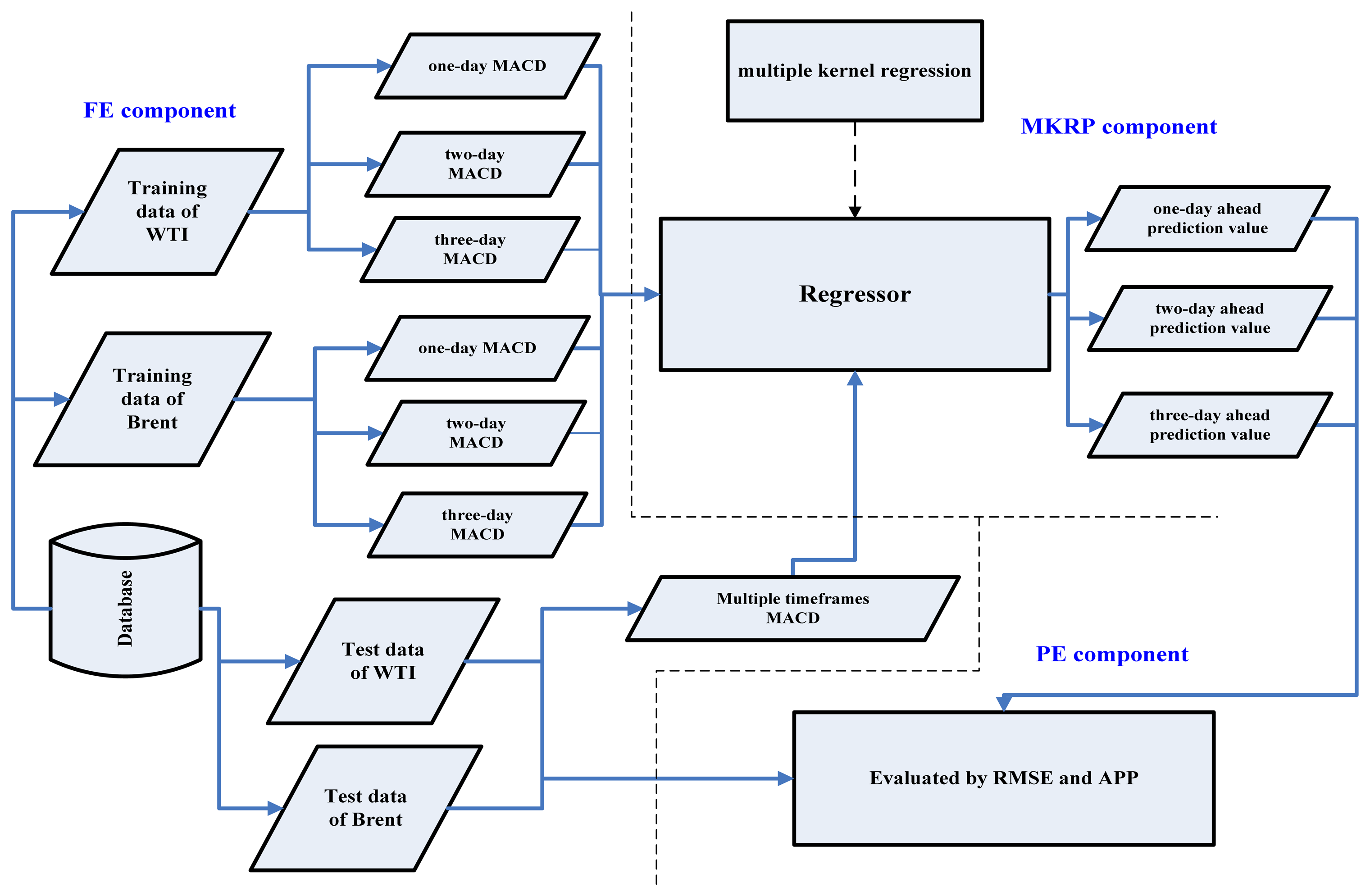
The proposed model is composed of three components as shown in Figure 1:
Feature extraction (FE) component;
Multiple kernel regression/prediction (MKRP) component;
Performance evaluation (PE) component.
The FE component first transforms crude oil spot price to MACD and MACD signals, following which it extracts features (historical n-days MACD features, see Table 1) from the two main crude oil markets and three different timeframes.
The MKRP component then predicts the crude oil price by fusing information from the two crude oil markets and three different timeframes. In this research, we have tested the forecasting ability of the proposed model on the basis of one-day, two-day, and three-day ahead predictions, while previous studies usually focused only on one-day ahead prediction.
For MKR, the input features are extracted from two different sources: WTI and Brent Crude oil prices. Since WTI and Brent Crude oil are the two biggest crude oil markets in the world, we selected these two sources.We transformed the original spot prices to MACD and MACD signal. For each kernel, the inputs are 4-period MACD values and MACD signals calculated from different timeframes. Details are presented in Table 1 and Figure 1.
Finally, the PE component evaluates the prediction and trading results based on the two evaluation criteria. This aspect is discussed in detail in Section 4.4.
4. Experimental Design
4.1. Research Data and Experiment Platform
There are a number of crude oil price series. Of these various series, two main crude oil price series, WTI crude oil spot price and Brent Crude oil spot price, are chosen as experimental samples. There are two primary reasons why these two are chosen as crude oil price sources for our study. First, these two crude oil markets have maximum impact on the world economy; hence, these forecasts would be useful for many countries in the world. Second, since fluctuations in one market could be an important reference for the other, both these markets have been used for the experiment. This study uses daily spot prices obtained from the energy information administration (EIA) website of the US Department of Energy (DOE) [28]. Note that this data includes only the spot price data for each working day.
The WTI crude oil spot price information we obtained from the website is from 2 January 1986 through 2 January 2012, and the Brent Crude oil spot price information is from 2 January 1987 to 2 January 2012. The difference in duration for which data was collected is because of reasons pertaining to data availability—the EIA website provides Brent data from 20 May 1987. Moreover, since this study uses information from both sources for prediction of price series, for reasons of convenience, we have considered data for the period ranging from 2 January 1990 to 31 December 2011, in both cases. Details of training and testing period are described in the Section 4.2.
In addition, in Section 5.4, we will show the experiment results by using information from crude oil markets (WTI and Brent crude oil markets), but also from two types of conventional gasoline market: “New York Harbor Regular” and “US Golf Coast Regular”. We selected these two additional oil markets because their history data is as early as that of Brent and WTI (from year 1986). Their data were downloaded from EIA website. The platform for experiment is Ubuntu, R language. MKL shogun package [27] is installed for MKL experiments.
4.2. Data Sets and Multiple Step-Ahead Predictions
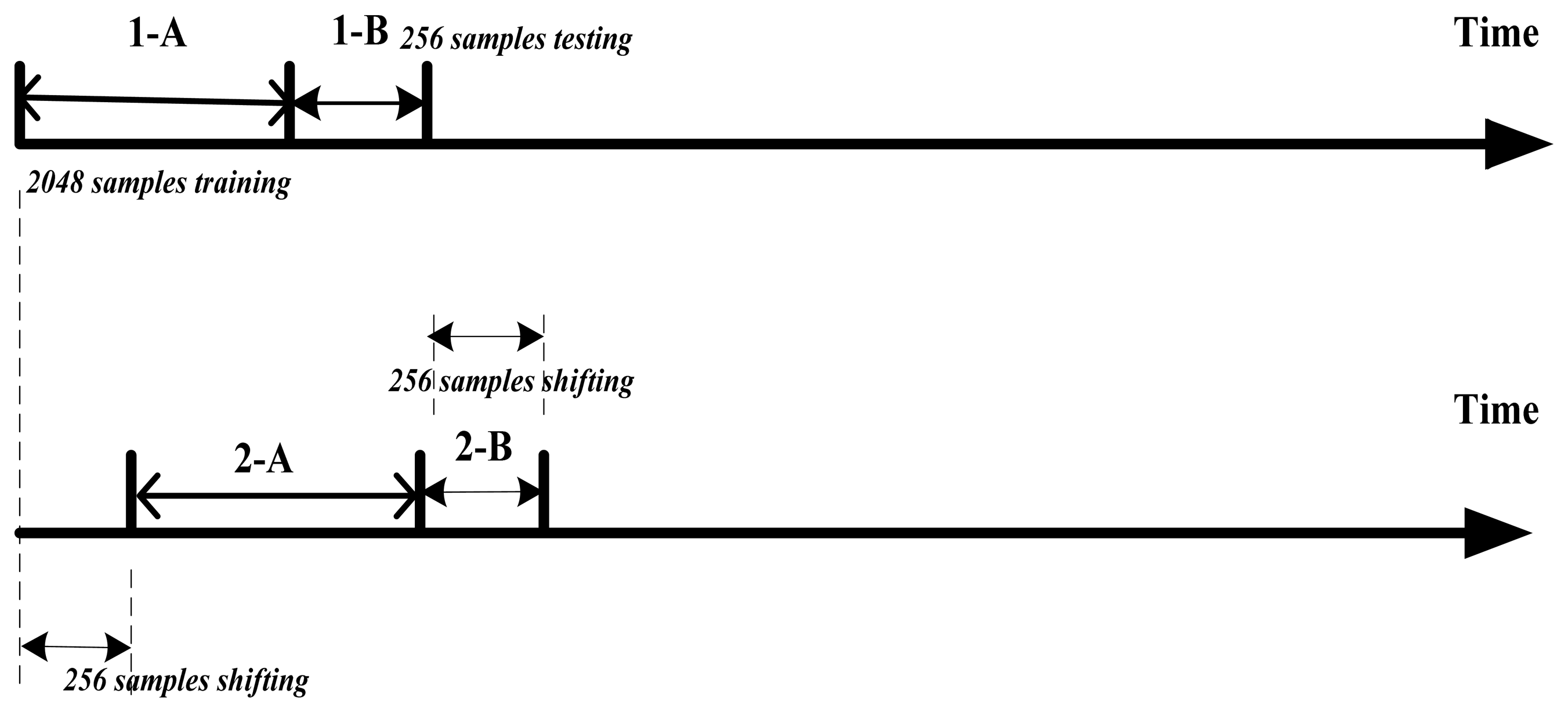
We used a rolling window method to separate the training and testing period. Since we want to have about 10 to 20 pairs of training and testing data and about one year for testing in the experiments, we decided to perform regression on data relating to 2048 trading days (around eight years) and obtained predicted values for 256 trading days (around one year). Further, for each subsequent experiment, we moved both the training and testing period forward by 256 trading days (around one year). There is a total of 14 training and testing periods for WTI and Brent crude oil price prediction from the beginning of 1990 to the end of 2011. The training and testing period and their relations are shown in Figure 2.
Additionally, we tested the prediction ability of the proposed model by conducting forecasts for three different days: one-day, two-day, and three-day ahead predictions. For example, for testing two-day ahead prediction, we predict the crude oil price two days later; for trading, we hold the trading position for two days and close the position after two days.
4.3. Proposed and Benchmark Methods
A list of proposed and benchmark methods is shown in Table 2. We use the term benchmark method to indicate high performance in case of a commonly used method. In the following list, MKR-M-3 and MKR-S-3 are our proposed methods and others are benchmark methods. Method 1 uses SVR as the learner, but only one source is used (the features from Brent are used to predict Brent Crude oil price) and only one timeframe is considered (to predict price two-day ahead, features of two-day timeframe are used); Method 2, SVR-S-3, uses features from three different timeframes of the target crude oil source. Method 3 uses features from two crude oil markets and from all the three timeframes. Method 4 uses the MKR framework and only one data source, that is, the target crude oil market, and three different timeframes. Method 5 represents another application of our proposed model and uses the same features as Method 3, but applies a MKR framework to all the information. Method 4 can be compared with Method 5 to test whether the additional features from other relevant markets are useful for prediction or not. Since MKR-S-1 uses only target market and only the target timeframe, it is the same as method SVR-S-1.
4.4. Evaluation Measures
To judge the forecasting performances and evaluate accuracy of prediction, two evaluation measures are used: root mean square error (RMSE) and average percentage profit (APP).
RMSE is a frequently-used measure to calculate differences between the values predicted by a model or a predictor and the values actually observed. It is defined by the formula:
In addition to the magnitude measures, we also measure the usefulness of the prediction for making profits in trading. Suppose the predictor predicts the oil price will go up (Pi is larger than Ri), we take up a long position in the crude oil futures market. If the predictor predicts the crude oil price to go down (Pi is smaller than Ri), we take up a short position in the crude oil futures market. The APP is defined as follows:
Note that m denotes the steps of m-day ahead prediction (i.e., m = 2 is for two-day ahead prediction). APP could be a useful measure of profitability for international companies, especially oil companies, airplane companies, and government energy organizations. Note that we do not consider transaction costs when calculating APP because unlike “trading” in stock or FX trading, we assume that government organizations and international companies trade crude oil without brokers. In the experiments, we do not do margin transaction, so the APP is calculated without leverage.
5. Experimental Results and Discussion
5.1. Prediction Results for Brent Crude Oil
Tables 3 and 4 show the average RMSE/mean and standard deviation of RMSE/mean results for Brent crude oil price prediction. Similarly, Tables 5 and 6 show the average RMSE/mean and standard deviation of RMSE/mean results for WTI.
From average RMSE/mean results of the total 14 experiments conducted (“mean” is the average crude oil price in the corresponding testing periods), the results of experiments based on the MKR model (MKR-S-3 and MKR-M-3) showed the best prediction results (the lower the value, better the score in RMSE/mean). Additionally, we found that although the SVR-S-3 and SVR-M-3 use more features from more sources than SVR-S-1, forecasts of these methods is less accurate than SVR-S-1. In fact, SVR-S-3 has additional features of two more timeframes and SVR-M-3 has additional features of another crude oil market and two more timeframes. The reason for this could be that SVR has failed to fuse the information from different sources and/or different timeframes. On the contrary, the MKR based methods (MKR-S-3 and MKR-M-3) yield better results than SVR-based methods (SVR-S-1, SVR-S-3, and SVR-M-3), indicating that information from different sources and different representations are useful for predictions. Moreover, this also indicates that, the MKR-based prediction methods fused the entire information more effectively than SVR-based methods.
Furthermore, since average RMSE/mean of MKR-M-3 and MKR-S-3 are not very different, we can conclude that the additional data source other than the target is not very useful. Moreover, on observing the standard deviation results, we find that the results of MKR-S-3 and MKR-M-3 are smaller than that of SVR-S-1, SVR-S-3, and SVR-M-3 for different prediction days (one-day, two-day, and three-day ahead). This indicates that the MKR-based model not only outperforms the SVR based model in terms of the magnitude of prediction, but it also attains low volatility. Similar conclusions could be derived for WTI crude oil price prediction from results shown in Tables 5 and 6.
5.2. APP Results for Brent and WTI
Tables 7 and 8 show the APP results for Brent and WTI prediction. First, we focus on the APP results of SVR based methods (SVR-S-1, SVR-S-3, and SVR-M-3). For Brent, SVR-S-1 method yields average returns at about 0.24% per day for one-day ahead prediction, about 0.21% per day for two-day ahead prediction, and about 0.14% per day for three-day ahead prediction, which indicates that although SVR used features only from the target crude oil market and target timeframe, it is a promising method for making profits in crude oil trading. SVR-S-3 and SVR-M-3 used more information (features from another crude oil market or other timeframes, or both) than SVR-S-1, but they presented worse results than SVR-S-1. The reason for this could be that the SVR was unable to effectively fuse information from different sources or different representations. Similar conclusion could be derived from the APP results of WTI shown in Table 8.
We now focus on the results for varying time horizons. From Tables 7 and 8, we find that for trading from three different time horizons, proposed method (MKR-S-3 and MKR-M-3) yields the best average APP results (14 experiments overall). For example, from APP results of WTI, MKR-S-3 and MKR-M-3 yield about 1.3% for one-day ahead prediction, 0.54% for two-day ahead prediction, and 0.34% for three-day ahead prediction. Since the results of MKR-S-3 and MKR-M-3 are very close, we can say that the data source other than the target is not useful.
Next, we focus on the results of different trading horizons for the same method. Note that since APP refers to average percentage profit per day (see Equation (13)), APP results for different time horizons of the same method are comparable. For WTI crude oil, one-day ahead prediction yields best average profit per day for SVR-S-1, SVR-S-3, MKR-S-3, and MKR-M-3, and worst results for SVR-M-3. We can draw similar conclusions on observing the APP results for Brent Crude oil: across all methods, one-day ahead prediction yields the best average profit per day than two-day or three-day ahead prediction yield. However, we found that for Brent and WTI, MKR-M-3 and MKR-S-3 yields very close profits, which indicates that features from another market do not necessarily improve trading performance.
Finally, we compare the results of our proposed method for WTI and Brent. For WTI, proposed method MKR-M-3 yields about 1.30%, 0.55%, and 0.34% per day for one-day, two-day, and three-day ahead predictions, respectively. For Brent, it yields about 1.05%, 0.46%, and 0.28% per day for one-day, two-day, and three-day ahead predictions, respectively. This indicates that for each prediction based on time horizon, the proposed method produced better results when applied to WTI spot price, rather than Brent spot price.
5.3. MKR Coefficients for Brent and WTI Predictions
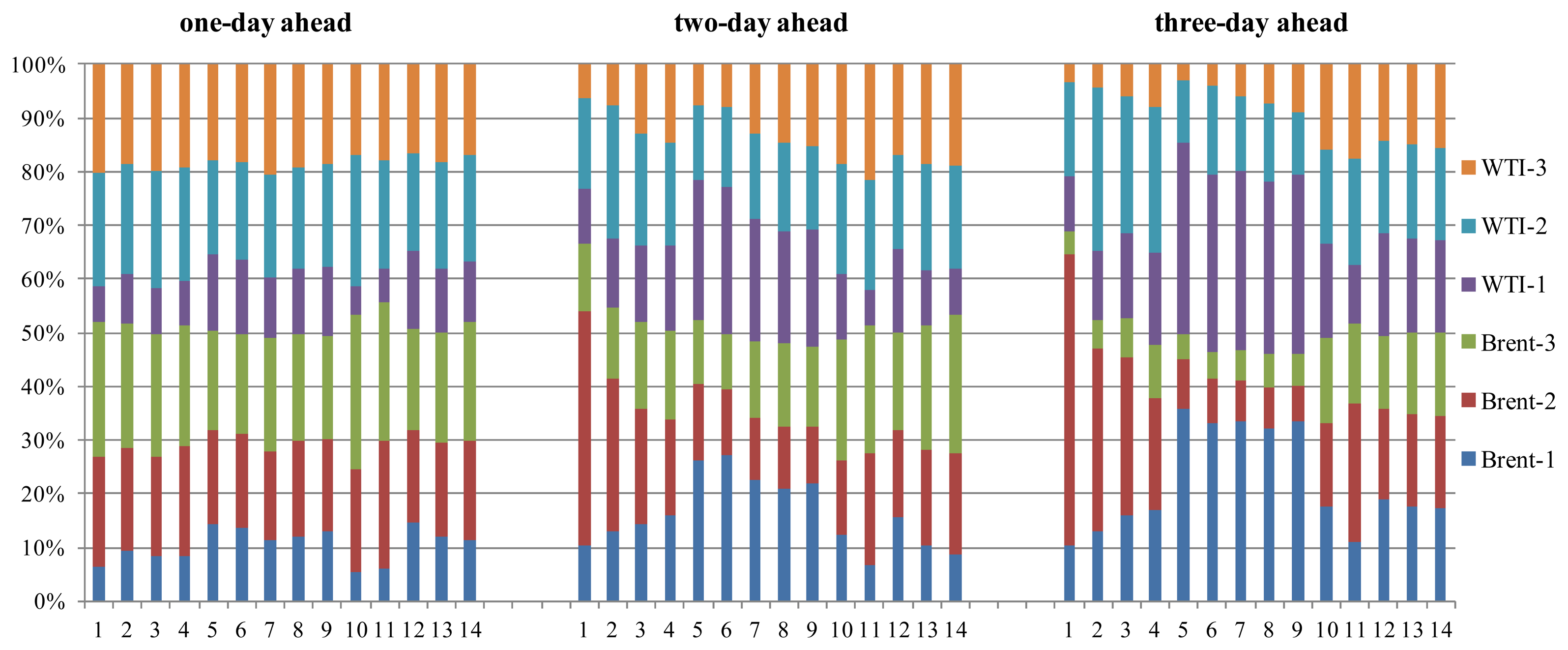
The coefficients for sub-kernels (βj in Equations (12)–(14)) are estimated in the MKR learning step, positive, and summed up to 1. Features adopted in sub-kernel with larger coefficient are considered as more important for the prediction than those in a sub-kernel with smaller coefficient, e.g., if the coefficient assigned to Brent-1 is 40% while the coefficient assigned to Brent-2 is 10%, it indicates that the features of Brent-1 is more influential than those of Brent-2 for prediction. In other words, the coefficients obtained using MKR show the possible correlation between the price movements in the target crude oil market with its target trading time interval and those in the other crude oil market with the same or other time horizons. Figures 3 and 4 show the coefficients of the kernel of MKR results for WTI and Brent crude oil price prediction in consecutive training periods. Since we have a total of 14 pairs (see Section 4.2) of learning and testing periods for each crude oil market, we have 14 sets of coefficient results for both markets. The y-axis in Figures 3 and 4 represents the relative values of coefficients of each feature set, and the x-axis represents the index of MKR training period. Labels of feature sets are expressed in short, as follows: for example, the label “Brent-3” means that the features are extracted from Brent Crude oil spot price by calculating MACD for a three-day timeframe.
For WTI one-day ahead prediction, we find that in most of the MKR training periods, the coefficients of Brent-2, Brent-3, WTI-2, and WTI-3 are larger than those of the others. Thus, it can be concluded that for predicting WTI crude oil price with one-day time horizon, features of Brent-2, Brent-3, WTI-2, and WTI-3 can be considered as more influential references than Brent-1 and WTI-1.
For two-day ahead prediction, the coefficient of WTI-2 drastically changes between training periods 4 and 5: while WTI-2 accounts for almost 35% in the 4th training period, it accounts for only 15% in the 5th training period, which is about a 20% point difference. The sudden coefficient change of WTI-2 indicates that the importance of WTI-2 features may have suddenly changed from the 4th to the 5th period for two-day ahead WTI prediction. We also observe that while coefficients of one-day timeframe features (Brent-2 and WTI-2) and three-day timeframe features (Brent-3 and WTI-3) decrease training period 4 onwards, the coefficients of one-day timeframe (Brent-1 and WTI-1), on the other hand, register an increase. This pattern indicates that the one-day MACD indicator feature gains relatively more importance for all subsequent training periods, after the 4th period.
For three-day ahead prediction, the coefficients of each feature set are not stable and coefficients of some feature sets, such as those of Brent-2 and WTI-2, change rapidly. This indicates that in case of predictions for longer time horizon, it is difficult to measure the relative importance of one feature over another as they demonstrate an unstable and dynamic character.
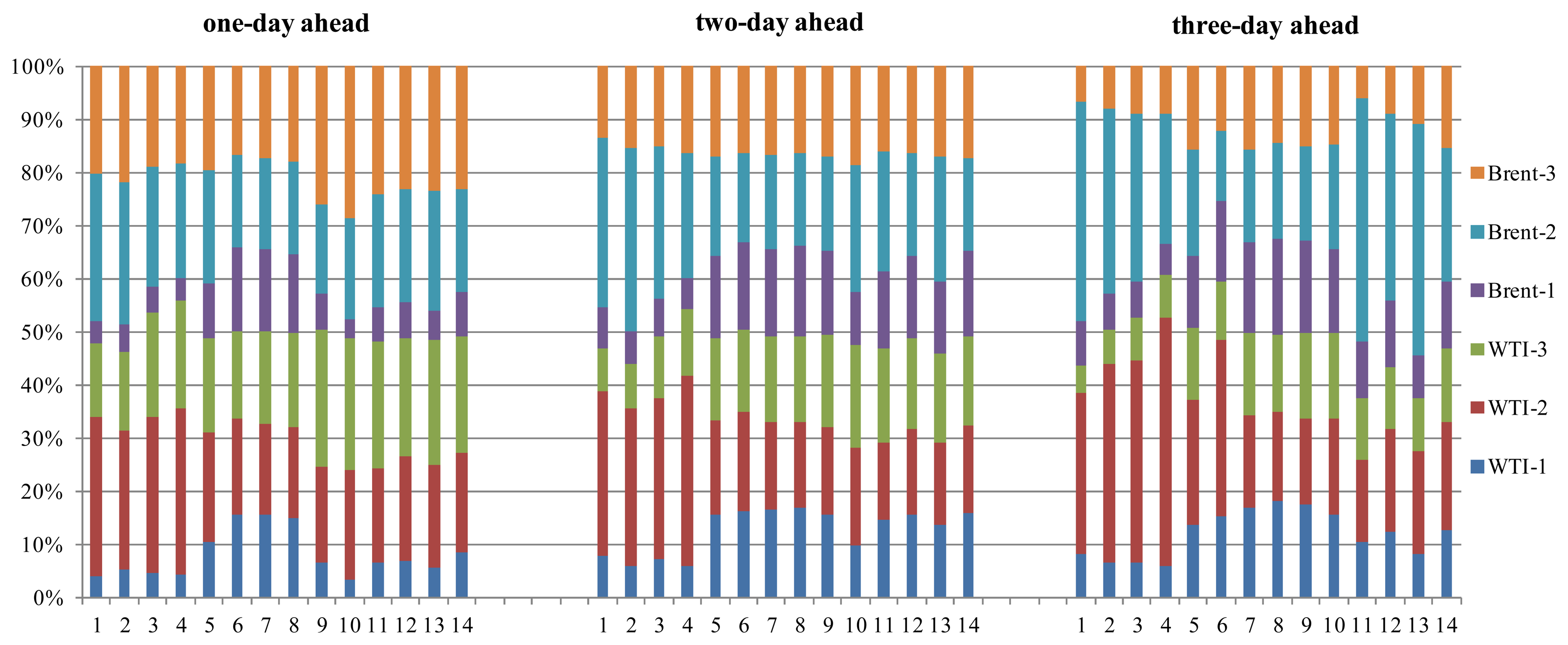
Figure 4 shows the coefficients of kernels of MKR results of each feature set for Brent Crude oil price prediction. Similar to the results observed for WTI one-day ahead prediction, coefficients of Brent-1 are stable during the 14 training periods. Additionally, Brent-1 and WTI-1 have relatively smaller coefficients than other longer timeframes. This may indicate that smaller trends are more impacted by features of longer timeframes.
For two-day ahead prediction, coefficients of some feature sets, especially Brent-1 and Brent-2, are not stable. As observed in the results for WTI, the coefficient of WTI-1 shows a sudden change from the 4th training period to the 5th training period.
For three-day ahead prediction, coefficients of many feature sets are not stable, and coefficients of more feature sets (than those of one-day and two-day ahead predictions), such as Brent-1, Brent-2, WTI-1, and WTI-2, change rapidly. This indicates, as it did in the previous case, that it is difficult to measure the relative importance of one feature over another in case of longer timeframes.
Moreover, from Figures 3 and 4, we find that the coefficients for one-day ahead prediction are more stable than that of two-day and three-day ahead predictions. The primary reason for this appears to be increasing uncertainty and unpredictability associated with longer timeframes, which produces suboptimal solutions in MKR, and this further resulted in one of such suboptimal solutions. We also observe that the APP results of one-day ahead prediction are better than those for two-day and three-day ahead predictions, which again could be attributed to the difficulty of predicting for longer time horizons.
In addition to the coefficients shown for consecutive experiment periods, Table 9 shows the average coefficients of MKR in these periods for one-day, two-day, and three-day ahead predictions, and Table 10 shows the standard deviation of the coefficients of MKR corresponding to Table 9. We can observe in Table 9 that for different crude oil markets or different time horizon predictions, the importance (in average) of each feature varies greatly. For example, for Brent three-day ahead prediction, Brent-1, Brent-2, WTI-1, and WTI-2, on average, account for around 20%, while Brent-3 and WTI-3 account for only about 9%. However, for Brent two-day ahead prediction, except WTI-3 (which accounts for about 13.8%), all other features obtained around 17%.
Additionally, we observed that for each prediction, the sum of coefficients of Brent (Brent-1, Brent-2, and Brent-3) and sum of coefficients of WTI (WTI-1, WTI-2, and WTI-3) are close to 50%. This indicates that for each prediction, the importance of both the crude oil sources is almost equal.
5.4. Results of Experiments using Information from Other Oil Markets
Tables 11 and 12 show RMSE results and APP results, respectively, of experiments using information from other oil markets. MKR-M-3 (proposed method) uses MKR as the learner and two crude oil sources (WTI and Brent crude oil) whereas MKR-F-3 uses MKR as the learner, but four oil sources (Brent, WTI, New York Harbor Regular, and U.S. Gulf Coast Regular) and three timeframes (1-day, 2-day, and 3-day ahead) are used. WTI-1, WTI-2, and WTI-3 are 1-day, 2-day, 3-day ahead prediction for WTI, respectively. Brent-1, Brent-2, and Brent-3 are 1-day, 2-day, 3-day ahead prediction for Brent, respectively. We conducted this experiment since we want to test whether the oil market information other than crude oil markets are useful or not for prediction of crude oil (WTI and Brent) prices.
From the average RMSE results shown in Table 11, we find that for three time horizons of WTI and three time horizons of Brent, results of MKR-M-3 and MKR-F-3 are very close to each other, which indicates that the increase of the other oil market information does not improve the prediction ability for WTI and Brent crude oil.
From the average APP results shown in Table 12, we find that MKR-M-3 outperforms MKR-F-3 for WTI-1, WTI-3, Brent-1 and Brent-3, while MKR-F-3 yields better APP results than MKR-M-3 for WTI-2 and Brent-2. It indicates the information from other oil sources does not always improve the profit making ability of the proposed model.
6. Conclusions
In this study, we have proposed an MKL-based crude oil prediction method, which includes three components: feature extraction (FE), multiple kernel regression for prediction (MKRP), and performance evaluation (PE). In this study, the FE component first extracts features as MACD indicator from two crude oil sources and three different timeframes. Second, the MKRP component predicts the crude oil prices by employing MKR. Finally, the PE component evaluates the prediction results by using RMSE and APP. Experimental results based on data from WTI and Brent Crude oil market show that MKR-based methods outperform benchmark methods on one-day ahead, two-day ahead, and three-day ahead predictions.
Experimental results show that prediction method based on the MKR framework yields better results than those obtained from SVR. Our study also detected that in case information is extracted from more than one source and/or different representations, SVR fails to effectively fuse the information, resulting in even more inaccurate results than those produced by employing the SVR method that used information from only a single source, pertaining to a single timeframe. On the contrary, methods based on the MKR framework effectively fused information from different sources and different representations, and produced better results than the benchmark methods, with the exception that the additional data source did not add to the effectiveness of the forecast. However, we first believed that the knowledge of another market price movements is beneficial for a trader (therefore we conducted experiments) but in fact, if the knowledge of one market price movement is highly utilized, the knowledge of another market price movement one day ago is not useful at least for the case we experimented. The reason might be that the two markets are correlated almost in real time.
The coefficients that we obtained from the MKL regression function for crude oil price prediction, using data from different crude oil markets and timeframes, demonstrated a possible correlation between our target crude oil market (WTI or Brent) and its target prediction time horizons (one-day, two-day, or three-day ahead), with other crude markets or other timeframes. The relative value of coefficients of the kernels in MKL results could be utilized to see possible correlations between reference crude oil markets with reference timeframes and the target crude oil market with the target prediction time horizon. As the time horizon goes on extending, coefficients of each feature set become unstable and the average percentage profit (APP) results become weak, indicating the difficulty with predicting crude oil price in longer time frames.
Future work in this field may take several interesting directions. For example, other than crude oil prices, stock prices of USA, main European stock markets, exchange rates of EUR/USD and USD/JPY are considered as useful information for predicting crude oil prices. Besides exploring some of these determinants of crude oil prices, possibility of incorporating features from more than three timeframes and including more stages in the step-ahead prediction model, could be investigated by future studies.
Acknowledgments
This research has been partially supported by Global-COE program (Symbiotic, Safe and Secure System Design program) of Keio University, Japan. The authors would like to thank their sponsors. Additionally, the authors would like to thank the EIA for making its crude oil spot prices data available, and authors of the MKL Shogun package, which greatly assisted in this research.
Conflicts of Interest
The authors declare no conflict of interest.
References
- Verleger, P.K. Adjusting to Volatile Energy Prices; Peterson Institute: Washington DC, USA, 1994; Volume 39. [Google Scholar]
- Taylor, M.P.; Allen, H. The use of technical analysis in the foreign exchange market. J. Int. Money Financ. 1992, 11, 304–314. [Google Scholar]
- Brock, W.; Lakonishok, J.; LeBaron, B. Simple technical trading rules and the stochastic properties of stock returns. J. Financ. 1992, 47, 1731–1764. [Google Scholar]
- Wong, W.K.; Manzur, M.; Chew, B.K. How rewarding is technical analysis? Evidence from Singapore stock market. Appl. Financ. Econ. 2003, 13, 543–551. [Google Scholar]
- Park, C.H.; Irwin, S.H. A reality check on technical trading rule profits in the US futures markets. J. Futures Mark. 2010, 30, 633–659. [Google Scholar]
- Aldea, C.E. Technical Analysis-Based Futures Trading System. Doctoral Dissertation, Simon Fraser University, Burnaby, BC, Canada, 1997; unpublished. [Google Scholar]
- Huntington, H. Oil price forecasting in the 1980s: What went wrong? Energy J. 1994, 15, 1–22. [Google Scholar]
- Gülen, S.G. Efficiency in the crude oil futures market. J. Energy Financ. Dev. 1998, 3, 13–21. [Google Scholar]
- Contreras, J.; Espinola, R.; Nogales, F.J.; Conejo, A.J. ARIMA models to predict next-day electricity prices. IEEE Trans. Power. Syst. 2003, 18, 1014–1020. [Google Scholar]
- Wang, T.; Yang, J. Nonlinearity and intraday efficiency tests on energy futures markets. Energy Econ. 2010, 32, 496–503. [Google Scholar]
- Haidar, I.; Kulkarni, S.; Pan, H. Forecasting model for crude oil prices based on artificial neural networks. Proceedings of the International Conference on Intelligent Sensors, Sensor Networks and Information Processing, ISSNIP 2008, Sydney, Australia, 15–18 December 2008; pp. 103–108.
- Yu, L.; Wang, S.; Lai, K.K. Forecasting crude oil price with an EMD-based neural network ensemble learning paradigm. Energy Econ. 2008, 30, 2623–2635. [Google Scholar]
- Wang, J.; Wan, W. Application of desirability function based on neural network for optimizing biohydrogen production process. Int. J. Hydrog. Energy 2009, 34, 1253–1259. [Google Scholar]
- Jammazi, R.; Aloui, C. Crude oil price forecasting: Experimental evidence from wavelet decomposition and neural network modeling. Energy Econ. 2012, 34, 828–841. [Google Scholar]
- Pierdzioch, C.; Rülke, J.C.; Stadtmann, G. New evidence of anti-herding of oil-price forecasters. Energy Econ. 2010, 32, 1456–1459. [Google Scholar]
- Pierdzioch, C.; Rülke, J.C.; Stadtmann, G. Oil price forecasting under asymmetric loss. Appl. Econ. 2013, 45, 2371–2379. [Google Scholar]
- Xie, W.; Yu, L.; Xu, S.Y.; Wang, S.Y. A new method for crude oil price forecasting based on support vector machines. Lect. Notes Comput. Sci. 2006, 3994, 441–451. [Google Scholar]
- Zhou, X.-L.; Wu, H.-W. Crude Oil Prices Predictive Model Based on Support Vector Machine and Particle Swarm Optimization. In Software Engineering and Knowledge Engineering: Theory and Practice; Springer: Berlin/Heidelberg, Germany, 2012; pp. 645–650. [Google Scholar]
- Bach, F.R.; Lanckriet, G.R.; Jordan, M.I. Multiple Kernel Learning, Conic Duality, and the SMO Algorithm. Proceedings of the Twenty-First International Conference on Machine Learning, Banff, AB, Canada, 4–8 July 2004; ACM: New York, NY, USA, 2004. [Google Scholar]
- Fletcher, T.; Hussain, Z.; Shawe-Taylor, J. Multiple Kernel Learning on the Limit Order Book. J. Mach. Learn. Res.-Proc. Track 2010, 11, 167–174. [Google Scholar]
- Luss, R.; D'Aspremont, A. Predicting abnormal returns from news using text classification. Quant. Financ. 2012. [Google Scholar] [CrossRef]
- Deng, S.; Mitsubuchi, T.; Shioda, K.; Shimada, T.; Sakurai, A. Multiple Kernel Learning on Time Series Data and Social Networks for Stock Price Prediction. Proceedings of the IEEE 10th International Conference on Machine Learning and Applications and Workshops (ICMLA), Honolulu, HI, USA, 18–21 December 2011; Volume 2, pp. 228–234.
- Yeh, C.Y.; Huang, C.W.; Lee, S.J. A multiple-kernel support vector regression approach for stock market price forecasting. Expert Syst. Appl. 2011, 38, 2177–2186. [Google Scholar]
- Vapnik, V. The Nature of Statistical Learning Theory; Springer: New York, NY, USA, 1995. [Google Scholar]
- Platt, J.C. Fast Training of Support Vector Machines Using Sequential Minimal Optimization. In Advances in Kernel Methods: Support Vector Machines; MIT Press: Cambridge, MA, USA, 1998. [Google Scholar]
- Sonnenburg, S.; Rätsch, G.; Schäfer, C.; Schölkopf, B. Large scale multiple kernel learning. J. Mach. Learn. Res. 2006, 7, 1531–1565. [Google Scholar]
- Sonnenburg, S.; Rätsch, G.; Henschel, S.; Widmer, C.; Behr, J.; Zien, A.; Franc, V. The SHOGUN machine learning toolbox. J. Mach. Learn. Res. 2010, 11, 1799–1802. [Google Scholar]
- U.S. Energy Information Administration. Available online: http://www.eia.doe.gov/ (accessed on 24 April 2014).


| No. | Feature | No. | Feature |
|---|---|---|---|
| 1 | MACD value at time t | 5 | MACD value at time (t − 2) |
| 2 | MACD signal at time t | 6 | MACD signal at time (t − 3) |
| 3 | MACD value at time (t − 1) | 7 | MACD value at time (t − 3) |
| 4 | MACD signal at time (t − 1) | 8 | MACD signal at time (t − 3) |
| No. | Method name | Data source | Timeframes | Prediction method |
|---|---|---|---|---|
| 1 | SVR-S-1 | Only the target market | Only the target timeframe | Support vector regression (SVR) |
| 2 | SVR-S-3 | Only the target market | Three timeframes | Support vector regression (SVR) |
| 3 | SVR-M-3 | Both the markets | Three timeframes | Support vector regression (SVR) |
| 4 | MKR-S-3 | Only the target market | Three timeframes | Multiple kernel regression (MKR) |
| 5 | MKR-M-3 | Both the markets | Three timeframes | Multiple kernel regression (MKR) |
| Method | One-day ahead | Two-day ahead | Three-day ahead |
|---|---|---|---|
| SVR-S-1 | 0.02796 | 1.99121 | 2.29711 |
| SVR-S-3 | 0.05688 | 3.34386 | 4.46337 |
| SVR-M-3 | 0.06629 | 5.17562 | 6.16460 |
| MKR-S-3 | 0.02316 | 1.60254 | 1.97642 |
| MKR-M-3 | 0.02316 | 1.60211 | 1.97584 |
| Method | One-day ahead | Two-day ahead | Three-day ahead | |
|---|---|---|---|---|
| SVR-S-1 | 0.01011 | 1.61699 | 1.76454 | |
| SVR-S-3 | 0.06187 | 2.68442 | 3.99079 | |
| SVR-M-3 | 0.02494 | 3.71164 | 4.43922 | |
| MKR-S-3 | 0.00447 | 0.95943 | 1.18787 | |
| MKR-M-3 | 0.00447 | 0.95845 | 1.18666 | |
| Method | One-day ahead | Two-day ahead | Three-day ahead |
|---|---|---|---|
| SVR-S-1 | 0.02856 | 2.02755 | 2.33543 |
| SVR-S-3 | 0.04904 | 3.49764 | 4.14796 |
| SVR-M-3 | 0.07788 | 5.83853 | 6.71285 |
| MKR-S-3 | 0.02450 | 1.70738 | 2.06678 |
| MKR-M-3 | 0.02450 | 1.70724 | 2.06662 |
| Method | One-day ahead | Two-day ahead | Three-day ahead |
|---|---|---|---|
| SVR-S-1 | 0.01050 | 1.47208 | 1.57962 |
| SVR-S-3 | 0.03186 | 3.20480 | 3.45841 |
| SVR-M-3 | 0.03384 | 4.58162 | 5.72177 |
| MKR-S-3 | 0.00510 | 1.05566 | 1.24878 |
| MKR-M-3 | 0.00510 | 1.05577 | 1.24895 |
| Method | One-day ahead | Two-day ahead | Three-day ahead |
|---|---|---|---|
| SVR-S-1 | 0.00242 | 0.00207 | 0.00138 |
| SVR-S-3 | −0.00132 | −0.00057 | −0.00036 |
| SVR-M-3 | −0.00154 | −0.00071 | −0.00040 |
| MKR-S-3 | 0.01038 | 0.00469 | 0.00282 |
| MKR-M-3 | 0.01054 | 0.00464 | 0.00280 |
| Method | One-day ahead | Two-day ahead | Three-day ahead |
|---|---|---|---|
| SVR-S-1 | 0.00367 | 0.00176 | 0.00117 |
| SVR-S-3 | 0.00057 | −0.00005 | 0.00009 |
| SVR-M-3 | −0.00143 | −0.00088 | −0.00044 |
| MKR-S-3 | 0.01390 | 0.00546 | 0.00344 |
| MKR-M-3 | 0.01309 | 0.00556 | 0.00348 |
| Target market and time horizon | Brent-1 | Brent-2 | Brent-3 | WTI-1 | WTI-2 | WTI-3 |
|---|---|---|---|---|---|---|
| Brent one-day | 0.10458 | 0.18613 | 0.21962 | 0.10458 | 0.20034 | 0.18471 |
| Brent two-day | 0.16146 | 0.18567 | 0.17001 | 0.16146 | 0.18291 | 0.13846 |
| Brent three-day | 0.21943 | 0.19276 | 0.09234 | 0.21943 | 0.18439 | 0.09163 |
| WTI one-day | 0.08025 | 0.20840 | 0.21438 | 0.08025 | 0.21686 | 0.19983 |
| WTI two-day | 0.12662 | 0.22418 | 0.16391 | 0.12662 | 0.20971 | 0.14893 |
| WTI three-day | 0.12008 | 0.27768 | 0.11531 | 0.12008 | 0.25153 | 0.11529 |
| Target market and time horizon | Brent-1 | Brent-2 | Brent-3 | WTI-1 | WTI-2 | WTI-3 |
|---|---|---|---|---|---|---|
| Brent one-day | 0.031287 | 0.019009 | 0.031188 | 0.031287 | 0.018160 | 0.012432 |
| Brent two-day | 0.066042 | 0.087793 | 0.048502 | 0.066042 | 0.029628 | 0.048715 |
| Brent three-day | 0.094199 | 0.131373 | 0.047001 | 0.094199 | 0.055894 | 0.053051 |
| WTI one-day | 0.043781 | 0.034358 | 0.035105 | 0.043781 | 0.050984 | 0.038125 |
| WTI two-day | 0.043023 | 0.057368 | 0.012079 | 0.043023 | 0.073336 | 0.034651 |
| WTI three-day | 0.043395 | 0.108578 | 0.035963 | 0.043395 | 0.100807 | 0.035932 |
| Method | WTI-1 | WTI-2 | WTI-3 | Brent-1 | Brent-2 | Brent-3 |
|---|---|---|---|---|---|---|
| MKR-M-3 (proposed method) | 1.22309 | 1.70724 | 2.06662 | 1.11768 | 1.60210 | 1.97584 |
| MKR-F-3 | 1.2223 | 1.70230 | 2.05287 | 1.11587 | 1.59464 | 1.95926 |
| Method | WTI-1 | WTI-2 | WTI-3 | Brent-1 | Brent-2 | Brent-3 |
|---|---|---|---|---|---|---|
| MKR-M-3 (proposed method) | 0.01309 | 0.00556 | 0.00348 | 0.01054 | 0.00464 | 0.00280 |
| MKR-F-3 | 0.00921 | 0.00578 | 0.00316 | 0.00778 | 0.00662 | 0.00211 |
© 2014 by the authors; licensee MDPI, Basel, Switzerland. This article is an open access article distributed under the terms and conditions of the Creative Commons Attribution license ( http://creativecommons.org/licenses/by/3.0/).
Share and Cite
Deng, S.; Sakurai, A. Crude Oil Spot Price Forecasting Based on Multiple Crude Oil Markets and Timeframes. Energies 2014, 7, 2761-2779. https://doi.org/10.3390/en7052761
Deng S, Sakurai A. Crude Oil Spot Price Forecasting Based on Multiple Crude Oil Markets and Timeframes. Energies. 2014; 7(5):2761-2779. https://doi.org/10.3390/en7052761
Chicago/Turabian StyleDeng, Shangkun, and Akito Sakurai. 2014. "Crude Oil Spot Price Forecasting Based on Multiple Crude Oil Markets and Timeframes" Energies 7, no. 5: 2761-2779. https://doi.org/10.3390/en7052761