1. Introduction
The permanent-magnet synchronous generator (PMSG), which is less noisy, high efficiency and has a long life span, has becomes one of the most important types of equipment in wind turbine systems. In 2008, Bumby designed and fabricated a 5 kW, 150 rpm axial vertical permanent-magnet (PM) generator driven directly by wind and a water turbine, where the generator uses trapezoidal shaped magnets to enhance the magnetism over conventional circular magnets. The average efficiency is 94% under no core losses and only limited eddy current loss [
1]. In 2011, Maia used finite element method (FEM) software to analyse the operation characteristics of an axial PM wind turbine with rated output power of 10 kW while running at the speed of 250 rpm [
2]. He [
3] indicated that the electromagnetic properties of the permanent-magnet machine are highly dependent on the number of slots per pole, phase, magnet shape, the stator slots and the slot opening. Eriksson described that a winding scheme having slots per pole ratio of 5/4 will reduce the cogging torque and suppress unwanted harmonics. The third harmonic distortion measured is 5.8% under no-load and load of a 12 kW direct driven PM synchronous generator [
4]. Erickson also designed a PM generator rated at 10 kW of telecommunication tower. The generator’s electrical efficiency is 94.3% using a 2-D FEM model simulation [
5]. From the literature to date, a systematic procedure and methodology concerning the determination of optimal structural parameters of PM wind generator leading to desired efficiency seems lacking. This motivated the study of this paper.
Axial flux PMSGs are widely used for vertical-axis wind turbines [
6,
7,
8,
9,
10], however, since the axial structure magnet is placed on the inner surface of the rotor without slot and facing the stator, it will lengthen the distance between upper and lower magnets, which in turn requires much more magnet material and cost to improve the operational efficiency.
This paper adopts the radial flux type PMSG, which has its stator windings placed in the inner core, needs less magnet, and therefore resulting in cost reduction as well as heat loss elimination. In addition, it applies vertical-axis wind turbine and direct drive structure and blade coupling generator. Therefore it doesn’t need to speed up/slow down the gearbox to decrease the noise caused and reduce the machinery wastage. It also presents a systematic approach for the design of permanent-magnet synchronous wind generator. To exemplify the feasibility of the proposed methodology, analysis and design of a high performance, multi-pole, gearless PMSG aiming at high efficiency and low voltage harmonics simultaneously using less material and having lighter structure is given. In addition, a novel six stator winding structure is also proposed to yield versatile applications. During low wind speed, the two three-phase windings are connected in series to increase the output voltage, while at high wind speed, the six windings are connected in parallel to provide more current and ensure power continuity when either one of the two three-phase windings fails [
11].
The paper is organized as follows:
Section 2 is concerned with the dimension of rotor design;
Section 3 describes the use of Maxwell 2-D to determine the suitable ratio of pole-arc to pole-pitch, and the use of the Taguchi method to find the stator-slot-shoes dimension; the designed parameters for high performance PMSG is also given in this section.
Section 4 presents experimental results and their comparison with Maxwell 2-D simulations; finally, conclusions are given in
Section 5.
2. Design Dimension of the Rotor
Both the designed double three-phase and six-phase winding configurations of PMSG consist of six composite windings with the advantage of high conductor utilization rate and lower torque ripple [
11]. Meanwhile, it can disperse the armature current evenly under the same voltage and power conditions.
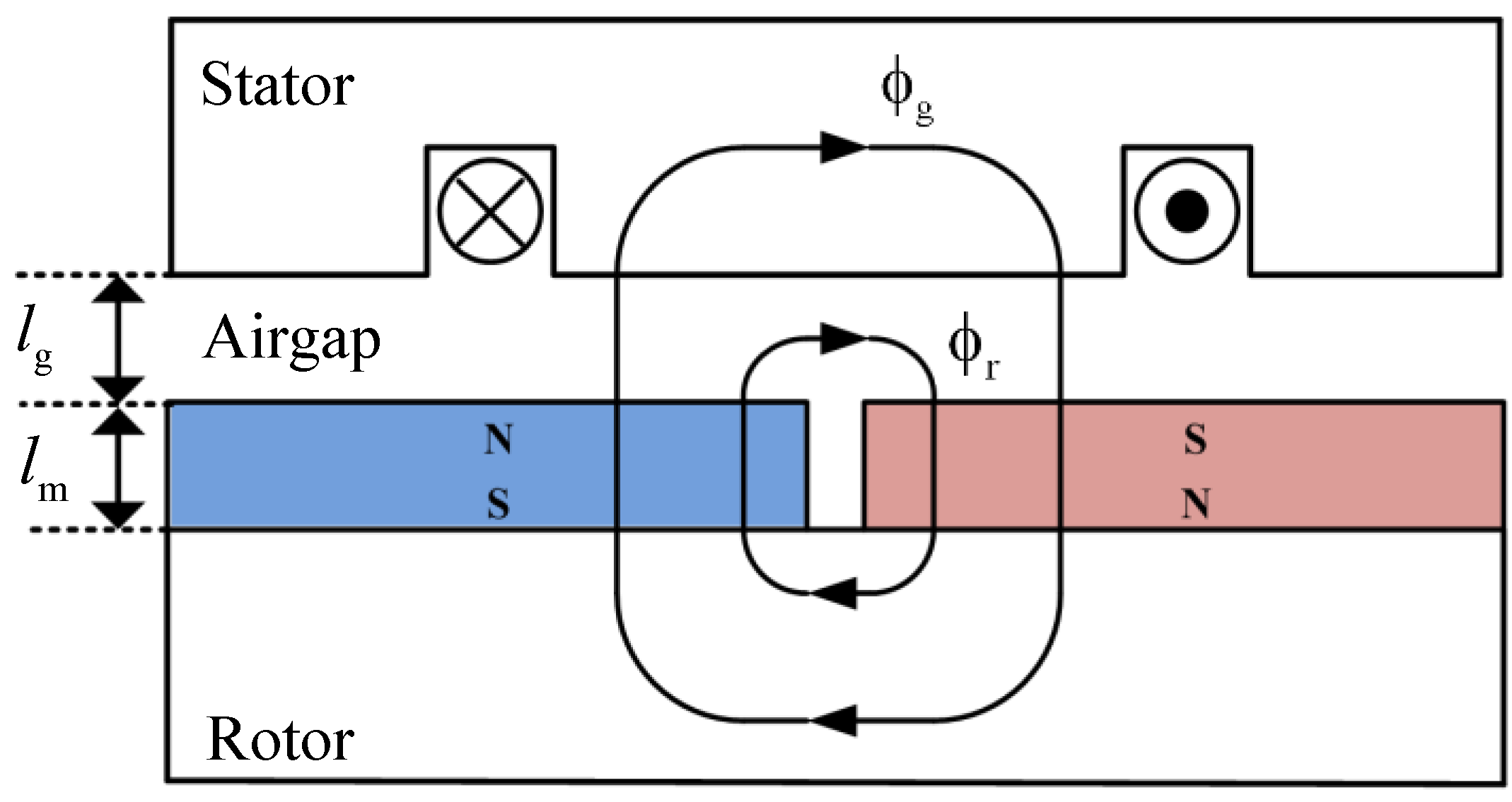
Figure 1 shows a simple and generally used surface mount with the basic geometric structure. It has a complete magnetic flux circuit, half N-pole and half S-pole, the magnetic flux travels from the rotor surface through the airgap, the magnetic silicon steel in the stator, the airgap, and then back to the rotor to form a complete closed-loop.
Figure 1.
Schematic diagram of permanent-magnet synchronous generator (PMSG): magnetic flux path.
Figure 1.
Schematic diagram of permanent-magnet synchronous generator (PMSG): magnetic flux path.
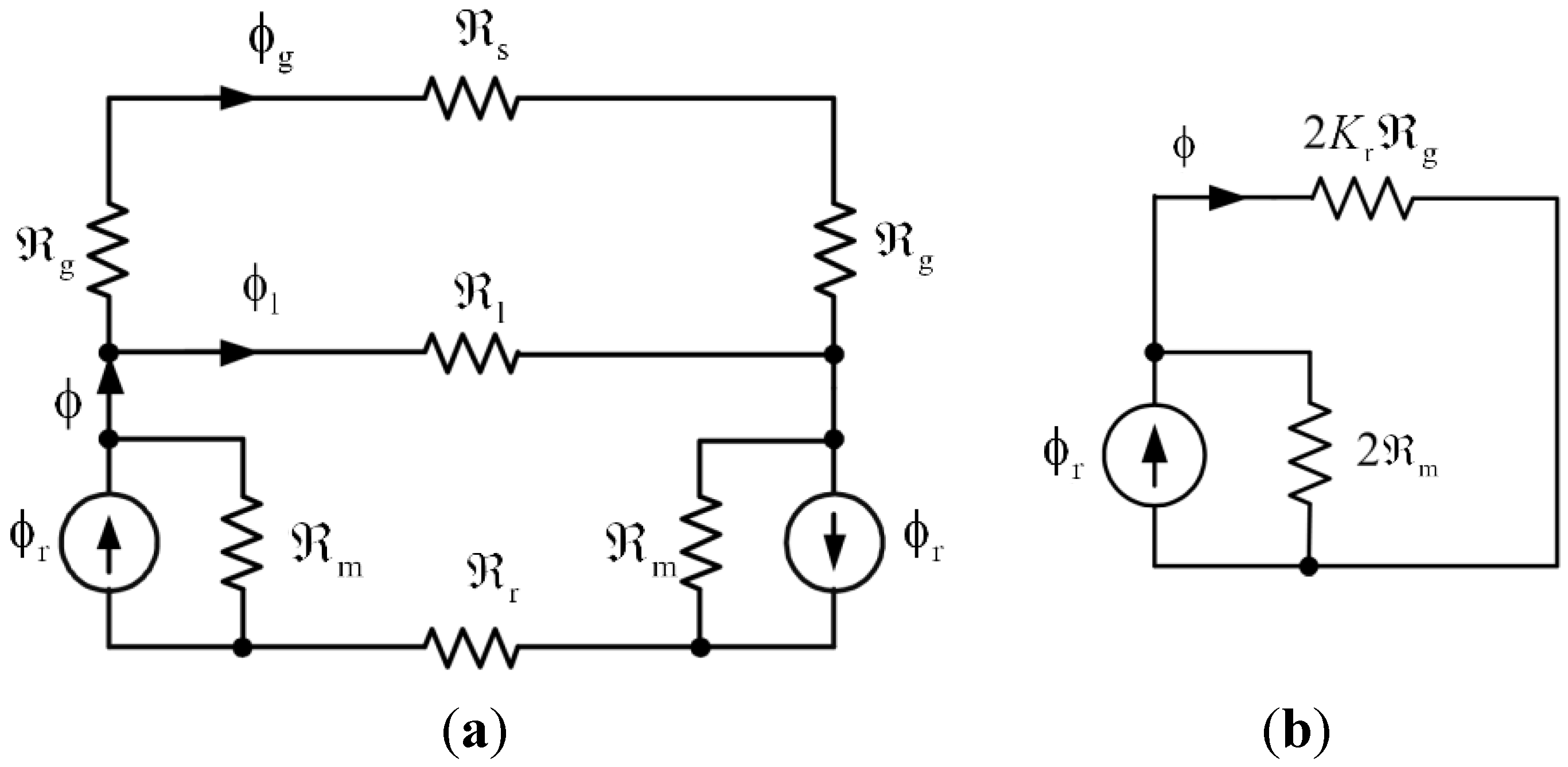
The equivalent magnetic circuit can be modeled as shown in
Figure 2a. The stator yoke width should be selected properly for reducing flux leakage and preventing magnetic saturation due to too small width of the yoke, or over weight and dimension coming from thicker yoke [
12].
Figure 2.
A magnetic circuit model for the proposed structure: (a) complete magnetic circuit model; (b) simplified magnetic circuit model.
Figure 2.
A magnetic circuit model for the proposed structure: (a) complete magnetic circuit model; (b) simplified magnetic circuit model.
The airgap flux can be written as ϕ
g =
Kl·ϕ, where the leakage factor
Kl is typically less than unity. For rapid analysis of the magnetic circuit, leakage magnetic reluctance
is ignored as shown in
Figure 2b. In addition, since the steel reluctance (
) is small relative to the airgap reluctance
, the steel reluctance can be eliminated by introducing a reluctance factor
Kr having its value chosen to be a constant slightly greater than unity to multiply the
to account for the neglected (
). For the machine with surface magnets under consideration, the leakage and reluctance factors are typically in the ranges of 0.9–1.0 and 1.0–1.2, respectively, while the flux concentration factor is ideally 1.0.
The magnetic flux can be derived as [
12]:
Since the relationship between permeance coefficient (
Pc) and airgap flux density is nonlinear, doubling
Pc does not double
Bg. Doubling
Pc, however, means doubling the magnet length, which doubles its volume and associated cost accordingly. Using the relation:
and:
Assuming that all the magnetic fluxes leaving the magnet through an airgap go into the stator core, then:
Since, as indicated above,
Kr is slightly greater than unity, it is further assumed that
Kr = 1. Thus, substituting Equation (5) into Equation (4) results in:
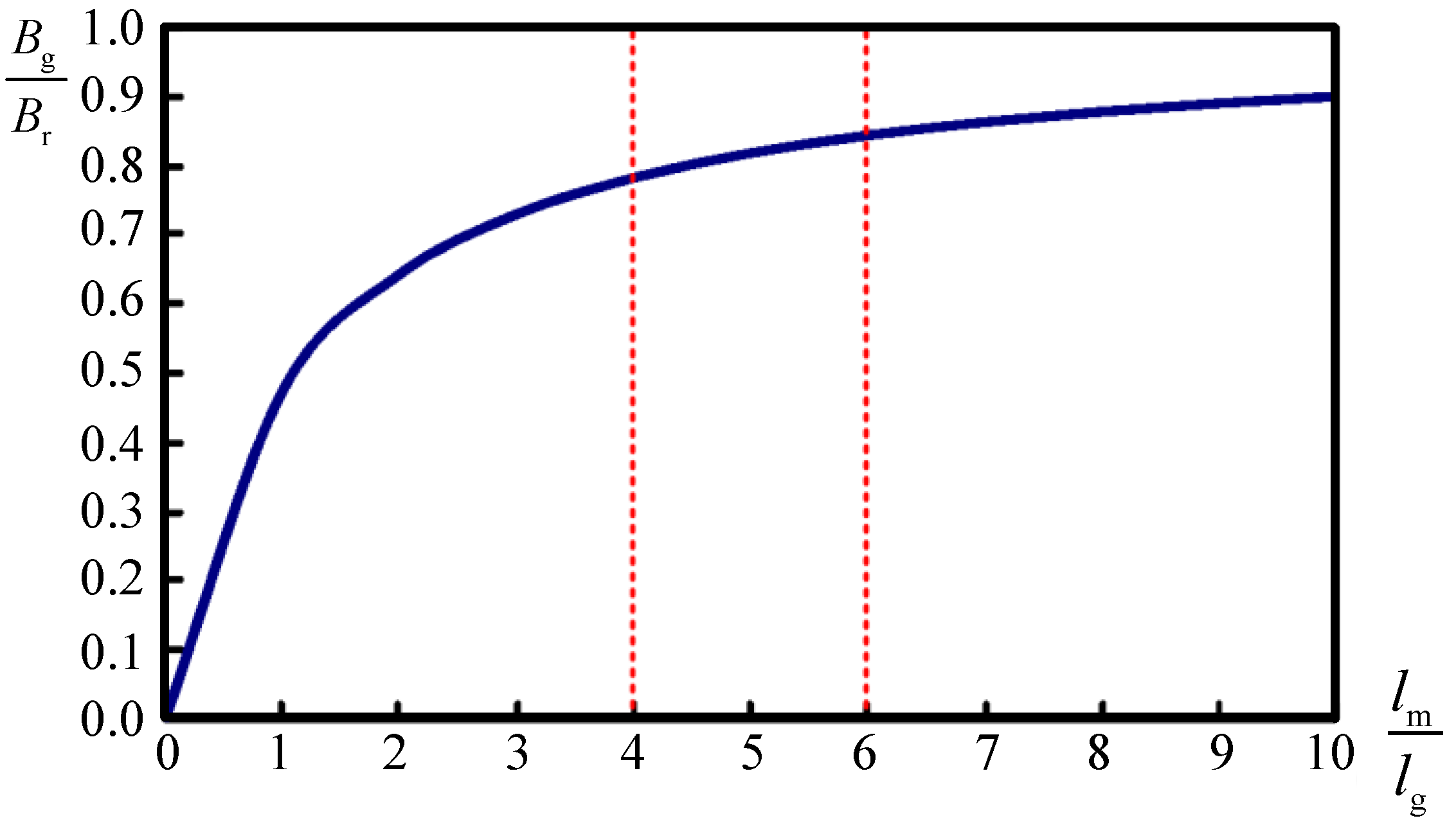
Determination of the airgap length
lg depends on the gap magnetic flux density and the processing of machine structure. If the airgap length is too short, it will cause serious eccentric force at high speed. Wider airgap length, however, will reduce the gap magnetic flux density and lower efficiency. The optimal ratio between magnet thickness and the airgap is usually selected in the range of 4–6 as shown in
Figure 3 [
12]. Usually generator designer determines magnet thickness in accordance with this search range. Meanwhile, production and installation tolerances must be considered to decide the eventual airgap length in order to avoid motor assembly complexity and operating problems. Equation (6) will be used to decide the initial airgap length shown in
Table 2 of
Section 3.
Figure 3.
Relationship between normalized airgap flux density and permeance coefficient.
Figure 3.
Relationship between normalized airgap flux density and permeance coefficient.
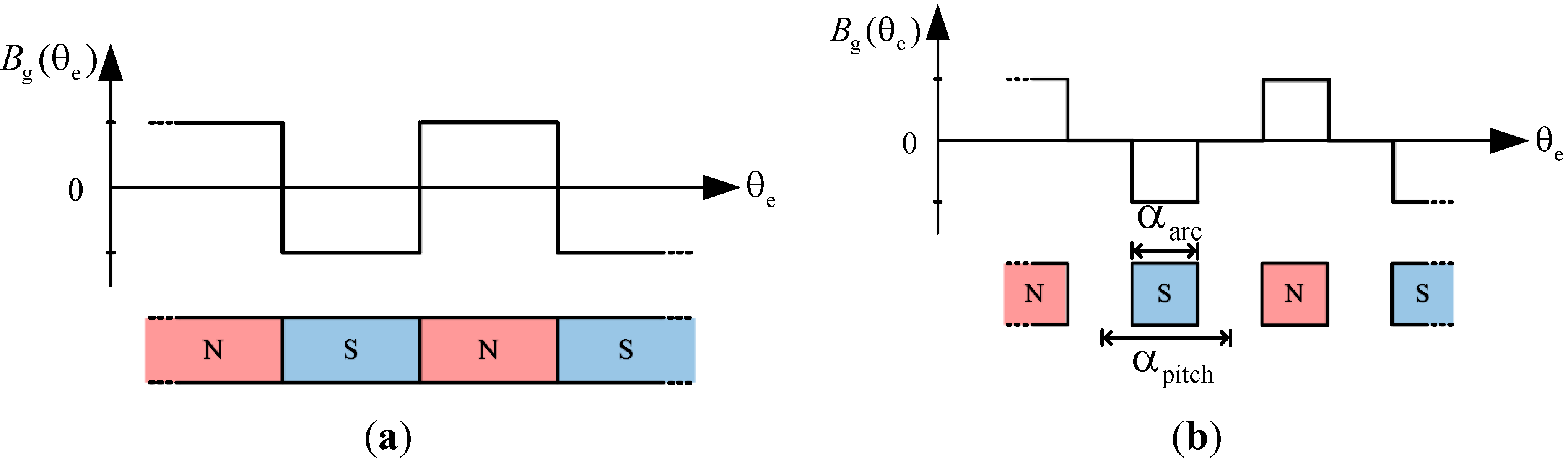
Ignoring the magnetic effects caused by the stator teeth, the distribution of airgap flux density can be illustrated by
Figure 4. The ratio α
p-p [
13] between the width of the magnet and the pole-pitch of rotor core, written as the ratio of pole-arc α
arc to pole-pitch α
pitch, is defined in Equation (7), where α
arc and α
pitch are the angular span of any single magnet and that between the center lines of any two adjacent magnetic poles, respectively. It is related to flux density. Specifically, the greater ratio,
i.e., the longer magnet arc length, will result in higher flux density. If the gap magnetic flux density waveform is closer to sinusoidal, then the induced voltage harmonics content will be smaller:
when α
p-p is unity, the N and S poles of the magnet are consecutive,
i.e., without a gap in between, the gap flux density is a square wave. In general, for 0 ≤ α
p-p ≤ 1, Fourier series expansion of the flux density at any electrical degree θ
e in the airgap can be derived as:
where
Bg,peak is the maximum flux density of airgap and
kh is the
k-th harmonic.
Figure 4.
Relationship between αp-p and airgap flux density: (a) αp-p = 1; (b) αp-p = 0.5.
Figure 4.
Relationship between αp-p and airgap flux density: (a) αp-p = 1; (b) αp-p = 0.5.
Equation (8) yields the
k-th harmonic flux ratio:
It is seen from Equation (9) that the airgap flux density ratio of harmonic is determined by different α
p-p, as shown in
Table 1. For balanced three-phase, the third harmonic can be eliminated by using Y-connected wiring. The harmonic distortion is not proportional to the phase and line voltages, but depends on the third harmonic of the phase voltage. Even if the third harmonic of the phase voltage will not appear in the line voltage, it will cause losses within each phase winding. It is obvious from
Table 1 that α
p-p = 0.800 will yield the smallest 3rd and smaller 5th harmonics. This choice of α
p-p for the smallest 5th harmonic will further be confirmed by the finite element analysis given in
Section 3.
Table 1.
Relationship between αp-p and airgap flux density ratio.
Table 1.
Relationship between αp-p and airgap flux density ratio.
| αp-p | | Harmonic content () |
|---|
| 1st (pu) | 3rd (pu) | 5th (pu) | 7th (pu) | 11th (pu) |
|---|
| 0.667 | 1.7322 | 0.8661 | 0.0000 | 0.1732 | 0.1237 | 0.0788 |
| 0.800 | 1.9022 | 0.9511 | 0.1960 | 0.0000 | 0.0840 | 0.0865 |
| 0.857 | 1.9498 | 0.9749 | 0.2605 | 0.0866 | 0.0000 | 0.0712 |
| 0.909 | 1.9796 | 0.9898 | 0.3032 | 0.1511 | 0.0771 | 0.0000 |
| 1.000 | 2.0000 | 1.0000 | 0.3333 | 0.2000 | 0.1429 | 0.0909 |
3. Simulation Results and Discussion
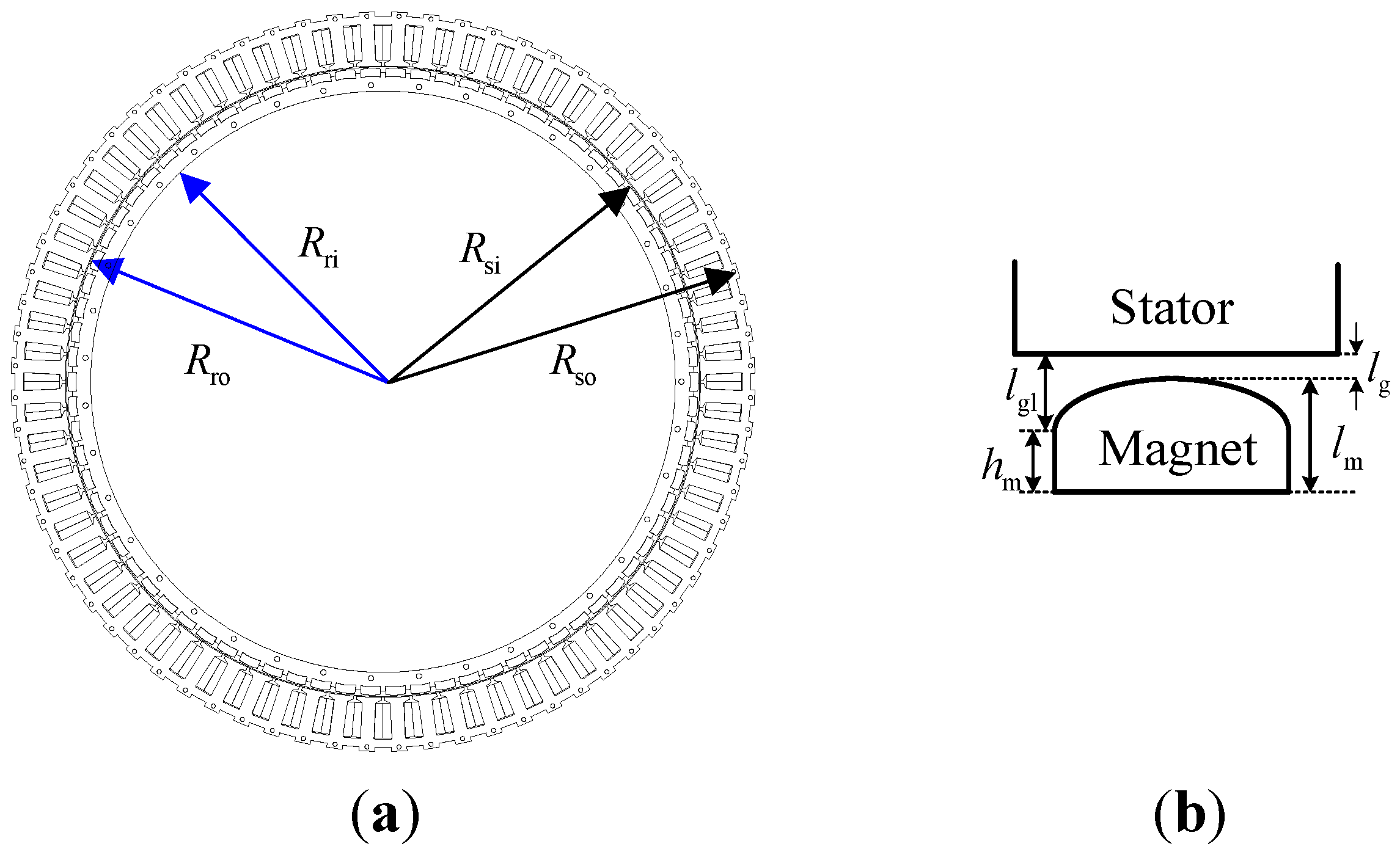
The finite element method from the Maxwell-2D software will be used throughout the analysis and design in this section. The relevant specifications and dimensions of the generator under design are listed in
Table 2 with the sketched schema graph of PMSG and magnet dimensions given in
Figure 5. As will be illustrated in the following, to design PMSG for double three-phase and six-phase winding connections, α
p-p will first be determined to obtain the greatest induced voltage and its smallest harmonic content.
Figure 5.
Schema graph of PMSG and magnet dimension: (a) structure of a 78-pole, 72-slot PMSG; (b) magnet dimension.
Figure 5.
Schema graph of PMSG and magnet dimension: (a) structure of a 78-pole, 72-slot PMSG; (b) magnet dimension.
The optimal size of the stator shoes is then decided by using the Taguchi method. Moreover, the induced voltage and current values can be determined by using different loads at the specific rotor speed and then calculate power output. Maxwell_2D and Fourier transform are applied to analyze PSMG-based electrical characteristics.
Table 2.
Parameters of wind generator to be designed.
Table 2.
Parameters of wind generator to be designed.
| Parameter | Value |
|---|
| Pole number | 78 |
| Slot number | 72 |
| Number of phase | double three-phase and six-phase |
| Rated speed (rpm) | 90 |
| Rated output power (W) | 10,000 |
| Rated torque (N·m) | 1,061 |
| Induced voltage (V) | 150 |
| Estimated efficiency (%) | 90 |
| Winding turns per slot (turns) | 25 |
| Winding conductor diameter (m) | (0.0012) × 4 |
| Stator radius: inner/outer (m) Rsi, Rso | 0.3065/0.3550 |
| Rotor radius: inner/outer (m) Rri, Rro | 0.2820/0.3045 |
| Airgap length (m) lg | 0.002 |
| Magnet thickness (m) lm | 0.008 |
| Stack length (m) | 0.12 |
| Core material/Permanent magnet | 50H400/NdFeB42H |
| End airgap length of rotor magnet (m) lgl | 0.0026 |
3.1. Optimal Sizing of Rotor Magnet
Aiming at high induced voltage and low harmonic distortion, sizing of rotor magnet will be conducted by the best pole-arc to pole-pitch ratio, α
p-p. Fixing the internal and external diameters of stator and rotor as given in
Table 2, double three-phase winding are used.
Assuming open stator slot as above, finite element analyses using Maxwell 2-D software for five different α
p-p,
i.e., α
p-p = 0.667, 0.800, 0.857, 0.909, and 1.000 are given.
Figure 6 shows the various phase voltage
Vp and line voltage
Vl values obtained by Maxwell 2-D with different α
p-p. When α
p-p = 0.800, the values for
Vp and
Vl are 243.3 V and 458.4 V, respectively.
Figure 6.
Induced voltages of PMSG with different αp-p by Maxwell 2-D: (a) Phase voltage; (b) Line voltage.
Figure 6.
Induced voltages of PMSG with different αp-p by Maxwell 2-D: (a) Phase voltage; (b) Line voltage.
The results shown in
Table 3 reveal that α
p-p = 0.800 will yield the smallest 5th harmonic voltage (0.14/0.13) with sufficiently high induced voltage. This agrees with
Table 1 that α
p-p = 0.800 will yield the smallest 5th and smaller 3rd harmonics. Besides, as mentioned in
Section 2 that for balanced three-phase, the third harmonic voltage can be eliminated by using Y-connected wiring.
Table 3.
Induced voltages and total harmonic distortion (THD) of 72-slot, 78-pole PMSG with different αp-p.
Table 3.
Induced voltages and total harmonic distortion (THD) of 72-slot, 78-pole PMSG with different αp-p.
| αp-p | Vp/Vl (V) | THD (%) | Each order harmonic (Phase/Line) |
|---|
| 3rd | 5th | 7th | 9th | 11th |
|---|
| 0.667 | 237.7/421.7 | 1.17/1.18 | 0.07/0.02 | 1.11/1.11 | 0.17/0.22 | 0.05/0.06 | 0.01/0.02 |
| 0.800 | 243.3/458.4 | 7.28/0.41 | 7.27/0.01 | 0.14/0.13 | 0.15/0.19 | 0.09/0.03 | 0.02/0.01 |
| 0.857 | 244.8/465.7 | 9.26/0.54 | 9.24/0.05 | 0.25/0.29 | 0.08/0.07 | 0.06/0.07 | 0.03/0.02 |
| 0.909 | 245.6/470.7 | 10.38/0.67 | 10.36/0.03 | 0.46/0.48 | 0.03/0.03 | 0.09/0.09 | 0.12/0.08 |
| 1.000 | 246.7/472.2 | 11.00/0.72 | 10.98/0.03 | 0.60/0.63 | 0.11/0.07 | 0.50/0.06 | 0.05/0.02 |
3.2. Determining the Optimal Stator-Slot-Shoes Dimension Using Taguchi Method
Conventionally, to find the most appropriate parameters for the optimum design, analyses or tests are usually conducted by changing one factor at a time for each experiment while other factors are kept fixed. The basic principle of Taguchi method is, however, to choose several control factors and use an orthogonal array to get useful statistic information with the fewest experiments. Taguchi method has been widely used in motor design since it provides engineers with a systematic and efficient method to administer numerical experiments and acquire the optimal parameters quickly [
14,
15,
16,
17,
18,
19,
20].
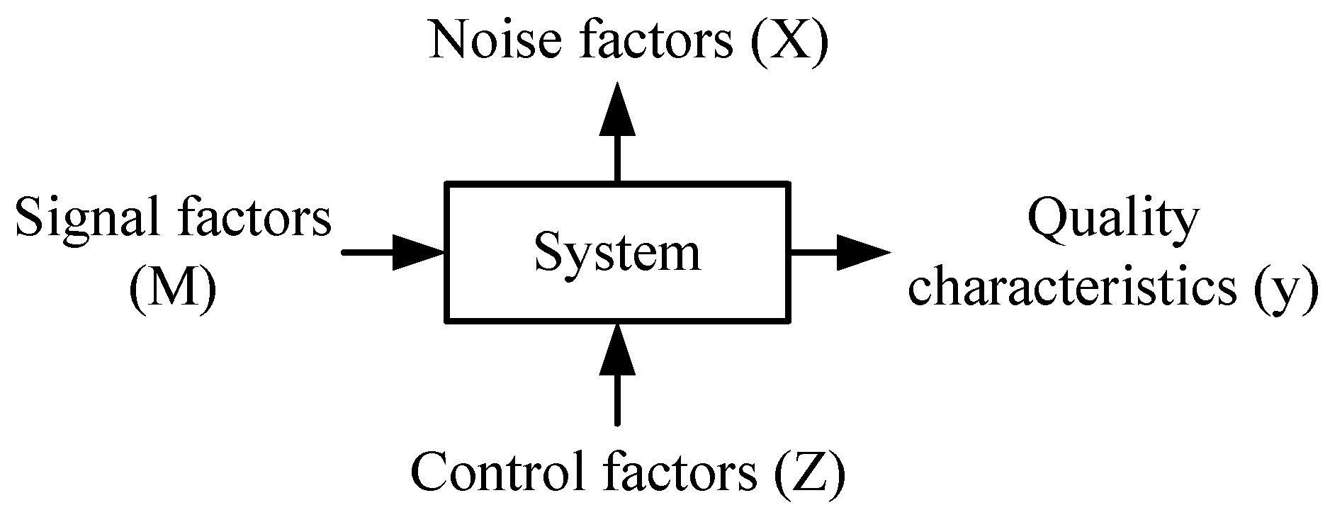
Consider the block diagram shown in
Figure 7, where system represents a product or manufacturing process, such as PMSG in our case here, y refers to the quality characteristics or response, signal factors (M), controllable factors (Z) and noise factors (X) are factors that can affect y [
16].
Figure 7.
Product/process parameters.
Figure 7.
Product/process parameters.
The effect of many different parameters or control factors on the performance characteristic in a condensed set of experiments can be examined by using the orthogonal array experimental design proposed by Taguchi [
14,
15]. Knowing the number of parameters and the number of levels, the proper orthogonal array can be selected as shown in
Table 4, which is adopted in this paper with the slot opening length, the height of the shoe portion, the magnet length, and the tooth width chosen as the control factors.
Table 4.
Array.
Table 4.
Array.
![Energies 07 07105 i001]() | Experiment | 1 | 2 | 3 | 4 | 5 | 6 | 7 | 8 | 9 | 10 | 11 | 12 | 13 | 14 | 15 | 16 |
| A | 1 | 1 | 1 | 1 | 2 | 2 | 2 | 2 | 3 | 3 | 3 | 3 | 4 | 4 | 4 | 4 |
| B | 1 | 2 | 3 | 4 | 1 | 2 | 3 | 4 | 1 | 2 | 3 | 4 | 1 | 2 | 3 | 4 |
| C | 1 | 2 | 3 | 4 | 2 | 1 | 4 | 3 | 3 | 4 | 1 | 2 | 4 | 3 | 2 | 1 |
| D | 1 | 2 | 3 | 4 | 3 | 4 | 1 | 2 | 4 | 3 | 2 | 1 | 2 | 1 | 4 | 3 |
| E | 1 | 2 | 3 | 4 | 4 | 3 | 2 | 1 | 2 | 1 | 4 | 3 | 3 | 4 | 1 | 2 |
One of the key features of Taguchi method is the use of signal-to-noise, S/N, ratio to transform the performance characteristic in the optimization process. The signal represents the mean performance while the noise signifies the variance. No matter what the applications, the method of measurement, or the units in which the results are expressed, there can be three types of S/N with the criteria: bigger is better, smaller is better and nominal is the best.
Taguchi strongly recommends the use of
S/
N ratio, expressed as a log transformation of the mean-squared deviation, as the yardstick for analysis of experimental results.
i.e.,
where the signal
g(
M;
Z) and the noise
e(
X;
M;
Z) are usually in the predictable and unpredictable sections, respectively. The objective of the design is to maximize the predictable and minimize the unpredictable parts, correspondingly.
For the-larger-the-better (LTB) target, the
S/
N ratio is:
For the-smaller-the-better (STB) quality characteristic,
S/
N ratio is defined as:
The performance index follows LTB for this paper, it can be expressed as:
The first mathematical term can be considered the induced voltage which in value is relatively higher; the next two terms respectively represent the total harmonic distortion (THD) and flux density of tooth width, both having a smaller value.
As mentioned above, four control factors, namely that slot opening length, external height of shoes (Shoes’_ho), internal height of shoes (Shoes’ hi) and tooth width are chosen in spite of the fifth control factor [
21,
22]. Moreover, four levels are applied for each factor to maximize the induced voltage of generator and keep the flux density of stator teeth lying within the saturation point of their laminations. Details are given in the following section.
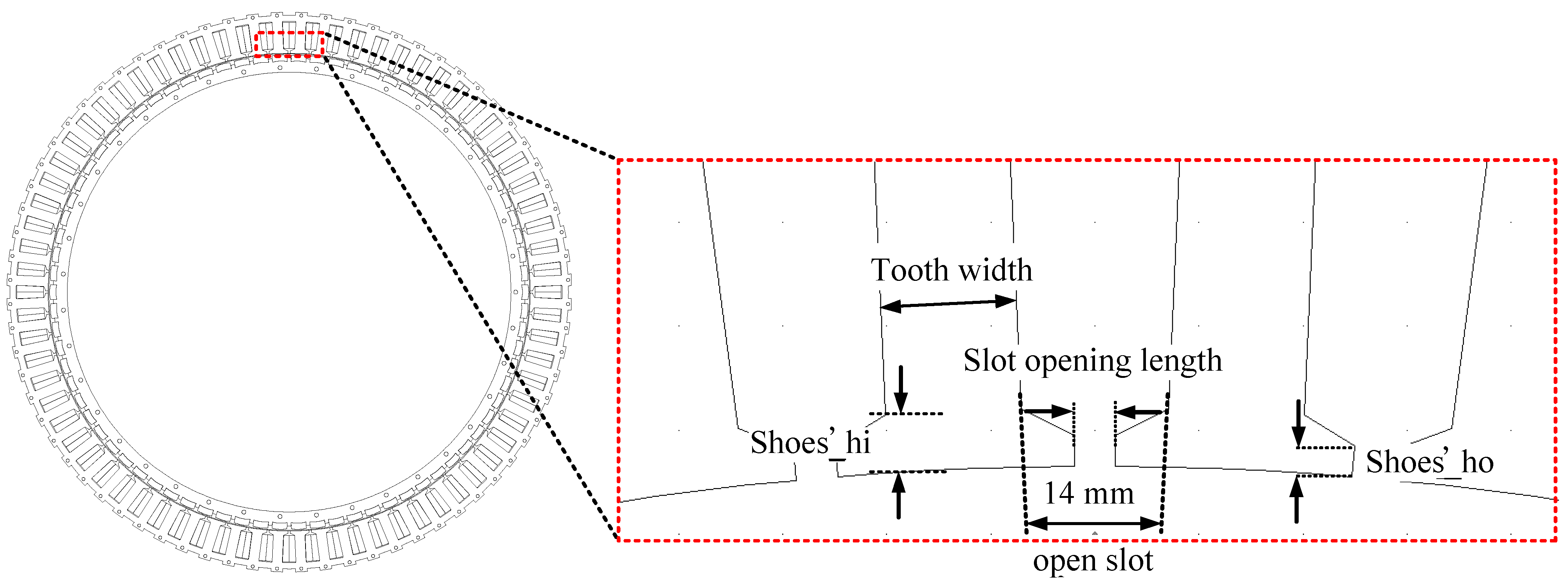
In this section, the Taguchi method will be used to determine the dimension of stator shoes. Consider
Figure 8. Four parameters, slot-opening length, ho, hi, and tooth width are chosen as control factors, which are subdivided into four levels to yield four row data shown in
Table 5 for the orthogonal array
L16(4
5) to process 16 simulations with Maxwell-2D and Matlab software. The results for no-load analysis of double three-phase winding configuration are summarized in
Table 6 and
Figure 9.
Figure 8.
Slot dimensions.
Figure 8.
Slot dimensions.
Table 5.
Four control factors and levels of stator shoes.
Table 5.
Four control factors and levels of stator shoes.
| Level | Control factor |
|---|
| A | B | C | D |
|---|
| Slot opening length (mm) | Shoes’_ho (mm) | Shoes’_hi (mm) | Tooth width (mm) |
|---|
| 1 | 1 | 0 | 1 | 7 |
| 2 | 2 | 1 | 2.5 | 9 |
| 3 | 3 | 2 | 4 | 11 |
| 4 | 4 | 3 | 5.5 | 13 |
Table 6.
Performance statistics for induced voltage, THD and flux density of tooth width. Optimized value: Vp(V): 208, THD(%): 0.39, TB: 1.2655, S/N: 52.49.
Table 6.
Performance statistics for induced voltage, THD and flux density of tooth width. Optimized value: Vp(V): 208, THD(%): 0.39, TB: 1.2655, S/N: 52.49.
| No. | 1 | 2 | 3 | 4 | 5 | 6 | 7 | 8 |
|---|
| Vp (V) | 149 | 163 | 191 | 207 | 179 | 185 | 158 | 186 |
| THD (%) | 1.58 | 2.69 | 1.71 | 0.65 | 1.84 | 2.85 | 3.83 | 2.18 |
| TB (Tesla) | 1.6489 | 1.5282 | 1.3050 | 1.2582 | 1.3491 | 1.2148 | 1.6823 | 1.5833 |
| S/N | 35.15 | 31.97 | 38.65 | 48.07 | 37.16 | 34.56 | 27.79 | 34.63 |
| No. | 9 | 10 | 11 | 12 | 13 | 14 | 15 | 16 |
| Vp (V) | 191 | 192 | 171 | 160 | 174 | 154 | 201 | 197 |
| THD (%) | 1.86 | 1.01 | 1.29 | 3.53 | 1.42 | 1.99 | 0.97 | 1.24 |
| TB (Tesla) | 1.2257 | 1.1457 | 1.5825 | 1.6956 | 1.5848 | 1.7199 | 1.2539 | 1.4692 |
| S/N | 38.46 | 44.40 | 38.46 | 28.54 | 37.77 | 33.06 | 44.36 | 40.68 |
Table 6 indicates that the best
S/
N ratio among the 16 simulations is obtained during the 4th run (
S/
N = 48.07), with
THD and
TB equal to 0.65 and 1.2582, respectively. Besides, It is seen from
Figure 9 that the dimensions of slot-opening length, Shoes’_ho, hi, and tooth width for the optimized
S/
N ratio are 4, 3, 5.5 and 13 mm, respectively; the corresponding optimized values are
Vp (V): 208,
THD (%): 0.39,
TB: 1.2655 and
S/
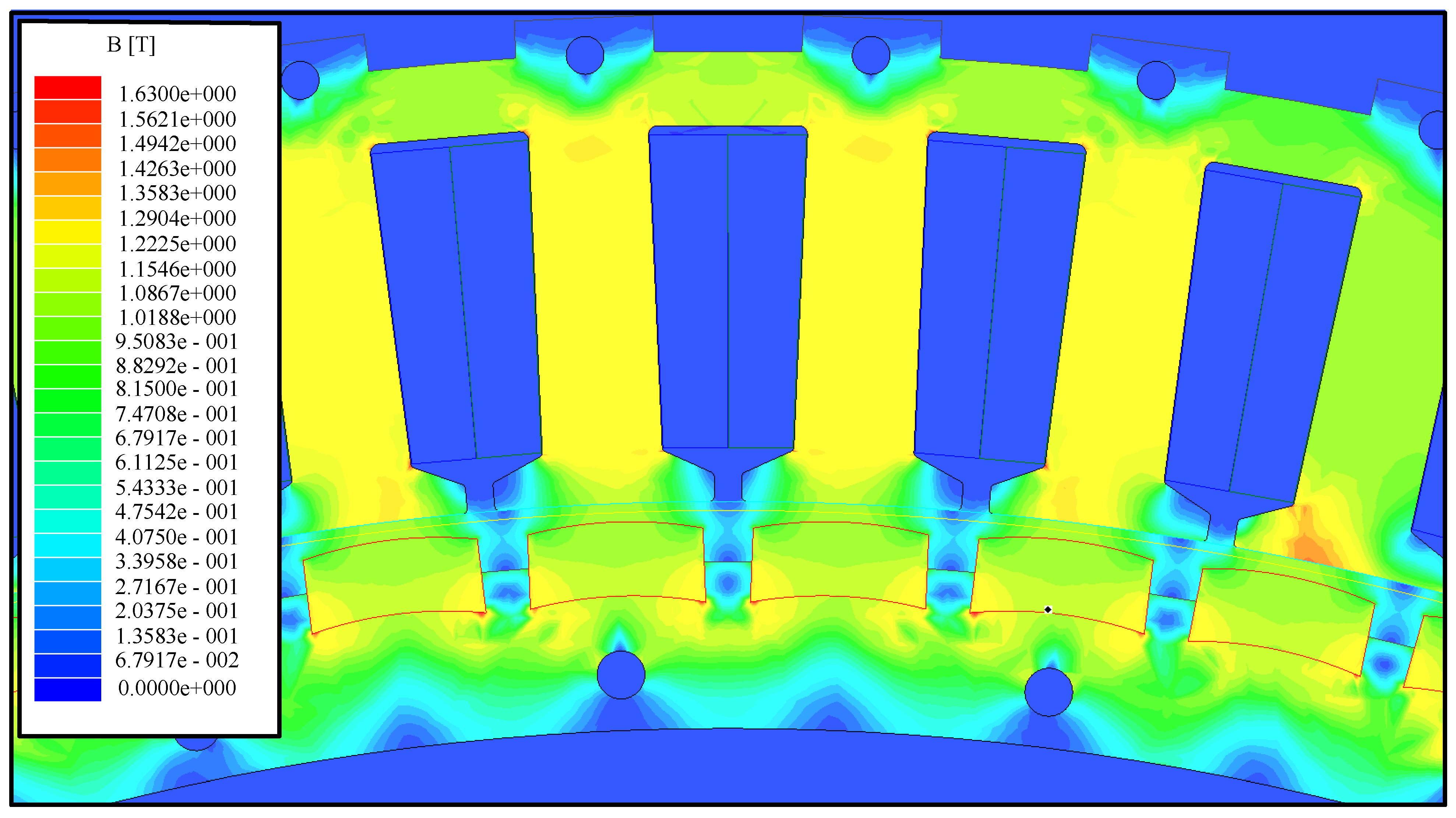
N: 52.49. When 50H400 silicon steel sheet is used with maximum saturation point, 1.6300 Tesla, as a limit, the optimized value from
Figure 10 (1.2655 Tesla) still does not exceed the threshold from simulations to avoid producing the problems of high temperature and the demagnetization phenomenon while the flux density of tooth width is near 1.6300 Tesla.
Figure 9.
Taguchi analysis for different control factors.
Figure 9.
Taguchi analysis for different control factors.
Figure 10.
Flux plot of the optimum stator-slot-shoes dimension by Maxwell-2D.
Figure 10.
Flux plot of the optimum stator-slot-shoes dimension by Maxwell-2D.
3.3. Finite Element Analysis of the Optimum Case
The electrical characteristics as mentioned refers to the analysis for the induced voltage, which may be further divided into the no-load and load tests. At different rotor speeds the corresponding induced voltage varies, and the rotor speed is proportional to the induced voltage. Furthermore, the induced voltage and current, as well as its output power can be determined at the specific rotor speed by using different loads. In this section, Maxwell-2D is used to analyze PSMG-based electrical characteristics. A Fourier transform with the results by using Matlab is then performed to obtain THD.
Based on the optimal parameters obtained above, finite element analysis with Maxwell-2D for 72-slot, 78-pole PMSG under seven different loads is conducted. The rotor is divided into two cylindrical segments of equal length, and adjacent segments are rotated on their axis by a constant angle of the generator. The results for induced voltages and
THD of double three and six phase winding configurations shown in
Table 7 indicate that
THD of both induced voltage and current are less than 1.4%, complying with IEEE Standard 519.
Table 7.
Simulated results by Maxwell-2D.
Table 7.
Simulated results by Maxwell-2D.
| Parameter | Vp (V)/THD (%) | Vl (V)/THD (%) | Ip (A)/THD (%) | Po (W) |
|---|
| Double three-phase winding | No load | 208 | 0.39% | 361 | 0.39% | - | - |
| Load 48 Ω | 205 | 0.31% | 355 | 0.31% | 4.3 | 0.33% | 2644.50 |
| Load 24 Ω | 199 | 0.31% | 345 | 0.31% | 8.3 | 0.31% | 4955.10 |
| Load 12 Ω | 182 | 0.33% | 316 | 0.33% | 15.2 | 0.33% | 8299.20 |
| Load 6 Ω | 146 | 0.38% | 252 | 0.38% | 24.3 | 0.34% | 10643.40 |
| Load 3 Ω | 95 | 0.82% | 164 | 0.86% | 31.6 | 0.28% | 9006.00 |
| Six-phase winding. | No load | 215 | 1.41% | 375 | 1.39% | - | - |
| Load 48 Ω | 212 | 1.20% | 355 | 0.31% | 4.4 | 1.24% | 2798.40 |
| Load 24 Ω | 206 | 1.08% | 356 | 1.05% | 8.6 | 1.08% | 5314.80 |
| Load 12 Ω | 188 | 0.95% | 336 | 0.90% | 15.7 | 0.95% | 8854.80 |
| Load 6 Ω | 149 | 0.63% | 258 | 0.64% | 24.9 | 0.63% | 11130.30 |
| Load 3 Ω | 97 | 0.36% | 167 | 0.84% | 32.0 | 0.36% | 9312.00 |
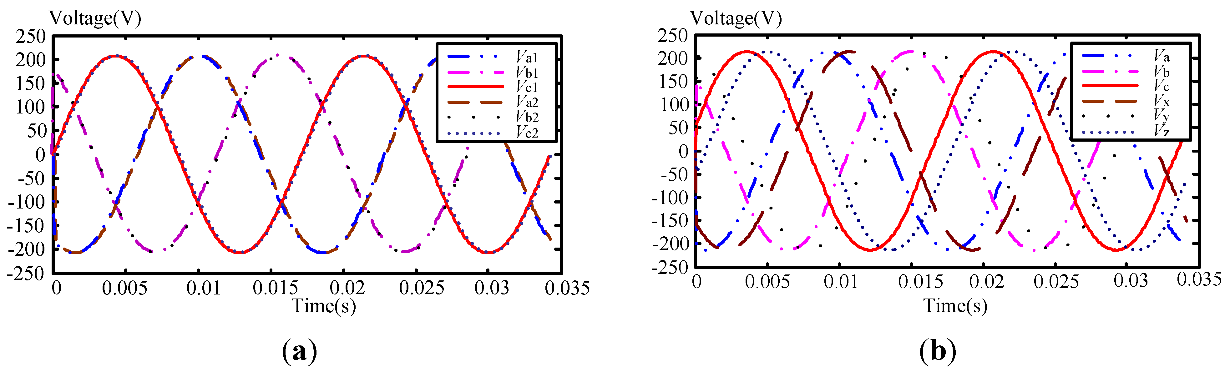
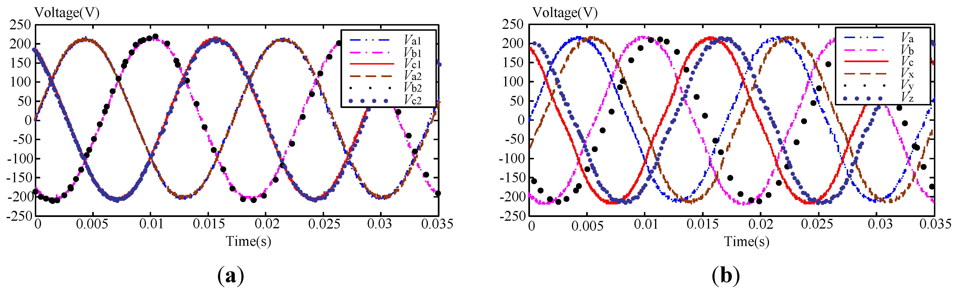
Figure 11 shows the induced voltages for the electrical angle equaling to 0° between
Va
1 and
Va
2 for the double three-phase winding; whereas the phase difference between
Va and
Vx phases is 30° for the six-phase winding. In addition,
Table 7 shows that
Vp are equal to 208 V and 215 V, respectively, for double three-phase winding and six-phase winding for no-load. This can also be verified from the near-sinusoidal voltage and current waveforms for no-load case from
Figure 11. When the speed is 90 rpm, from
Table 7, the 6 Ω load receives generator outputs of 10.643 kW and 11.130 kW for the double three-phase winding and six-phase winding, respectively.
Figure 11.
Analysis of induced voltage at no-load: (a) double three-phase winding; (b) six-phase winding.
Figure 11.
Analysis of induced voltage at no-load: (a) double three-phase winding; (b) six-phase winding.
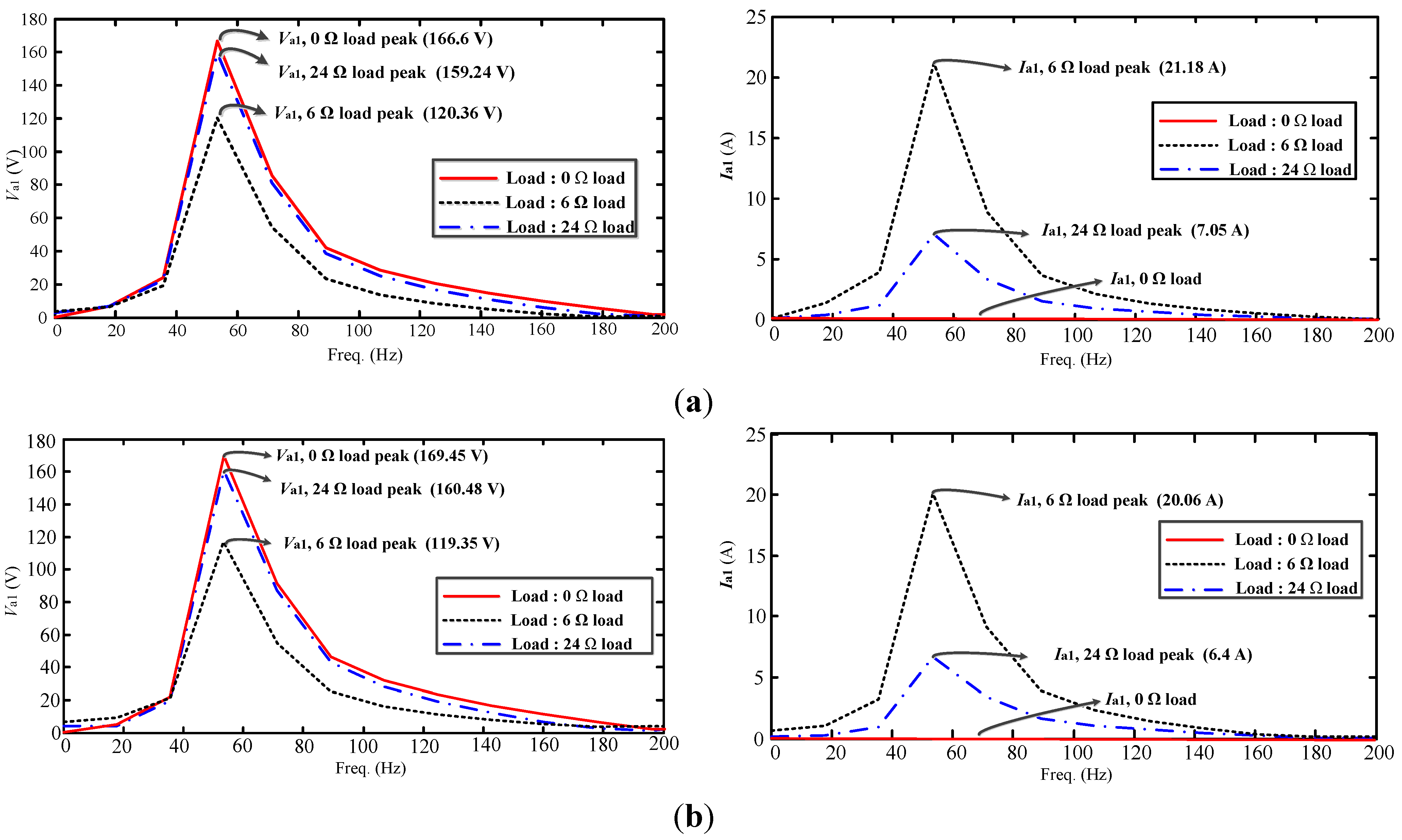
From the frequency domain analysis for
Va
1,
Figure 12 shows that the peak values for
Va
1 under 24 Ω load for the double three-phase winding and six-phase winding are 159.24 V and 160.28 V, respectively, with the corresponding peak values of 7.05 A and 6.43 A for
Ia
1.
Figure 12.
Induced voltage and current at 0, 6 and 24 Ω-load: (a) double three-phase winding; (b) six-phase winding.
Figure 12.
Induced voltage and current at 0, 6 and 24 Ω-load: (a) double three-phase winding; (b) six-phase winding.
4. Experimental Results and Discussion
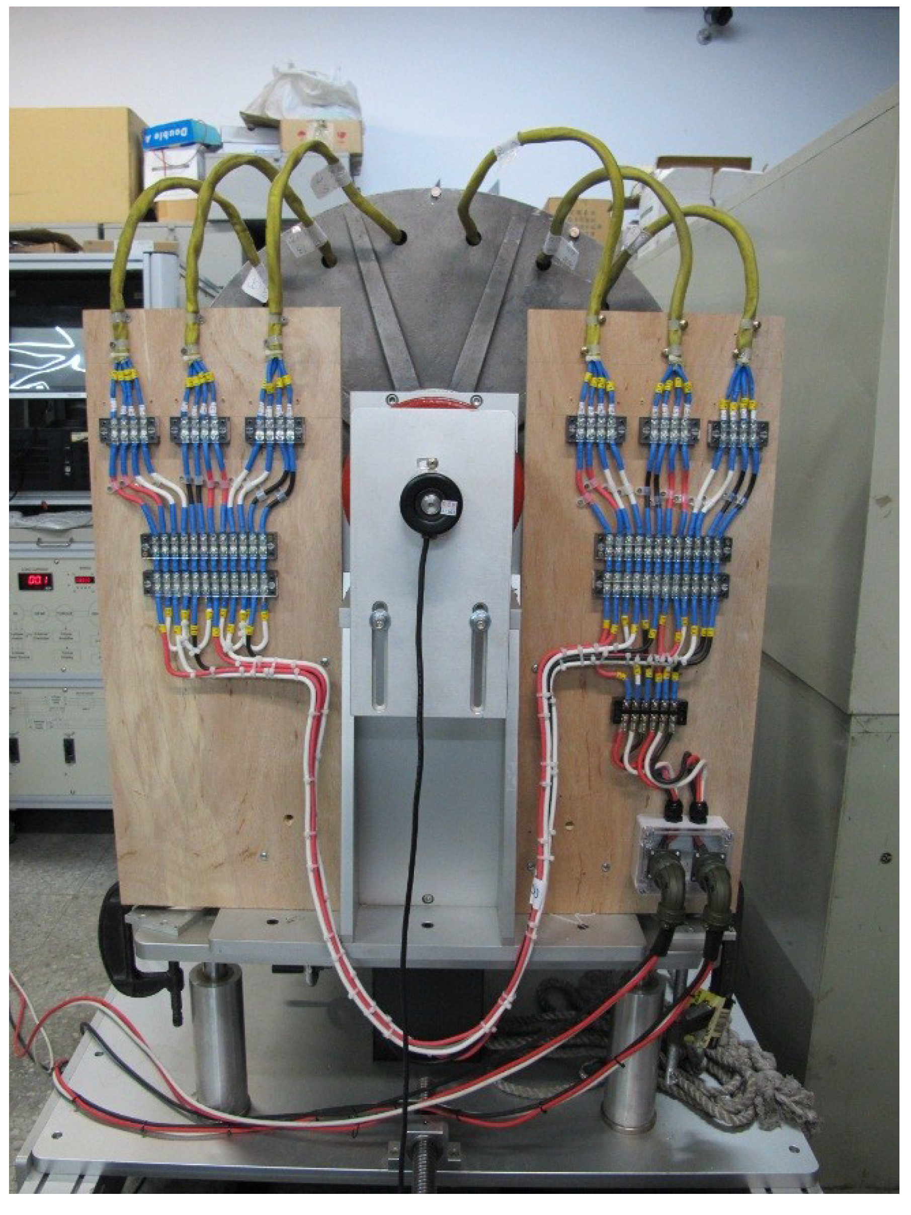
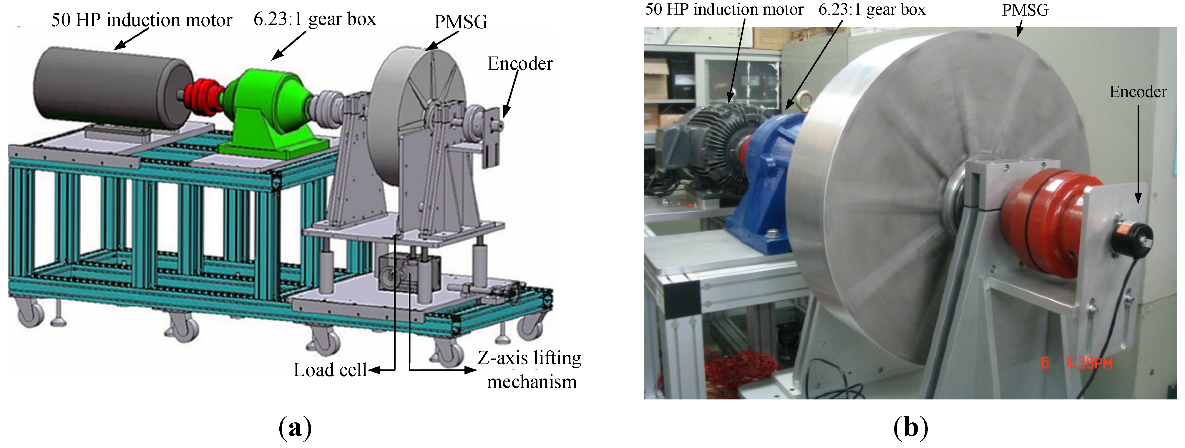
This section presents the experimental results conducted on the proposed high performance PMSG. The generator and its measurement platform are built and shown in
Figure 13, which contains a 6-pole, 50 horsepower (50 hp = 37.3 kW) induction motor as the prime mover.
Figure 13.
Experimental apparatus: (a) schematic diagram; (b) platform photo.
Figure 13.
Experimental apparatus: (a) schematic diagram; (b) platform photo.
It is seen from
Figure 13 that the 72-slot, 78-pole PMSG under test is driven via a reducer with speed ratio of 6.23:1. The wiring of double three-phase and six-phase winding configurations can easily be accomplished through the proposed scheme shown in
Figure 14. Calculation of powers and efficiencies using simulated results will be given to compare with the experimental evaluation in this section.
Figure 14.
External wiring photo.
Figure 14.
External wiring photo.
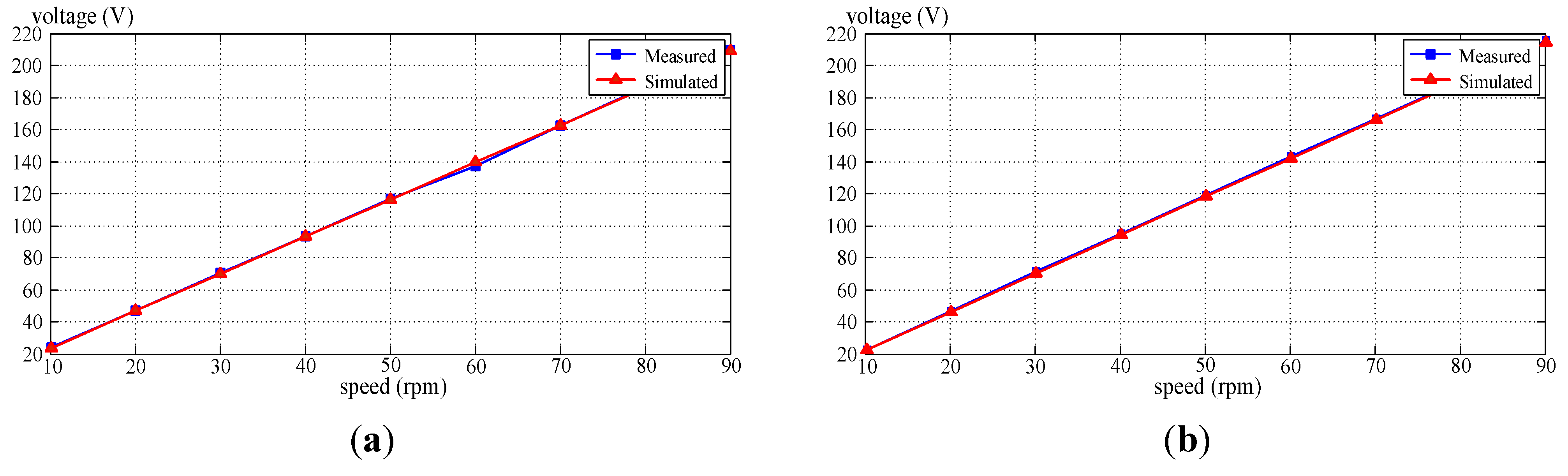
The measured and simulated induced voltages of the PMSG from no-load test for both winding configurations under different speeds are given in
Figure 15, where linear relationships between the induced voltage and speed are observed. Besides,
Figure 15 also reveals that close agreements for induced voltages between measured and simulated results are obtained. In fact, the differences for both wirings are less than 1%.
Figure 15.
Measured and simulated no-load induced voltages: (a) double three-phase winding; (b) six-phase winding.
Figure 15.
Measured and simulated no-load induced voltages: (a) double three-phase winding; (b) six-phase winding.
Since the maximum output power of the load box is 5 kW when the generator is operated at rated speed of 90 rpm, the experimental results can only be obtained and compared with simulations for the resistive load of 24 Ω. The experimental results under no-load and 24 Ω load shown in
Table 8 indicate that
THD of the induced line voltages are within 3% for both winding configurations, complying with IEEE Standard 519 as in the simulation case. The corresponding waveforms of the induced voltages given in
Figure 16 show near-sinusoidal outputs for no-load case.
Table 8.
Measured induced voltages and THD.
Table 8.
Measured induced voltages and THD.
| Parameter | Vp (V)/THD (%) | Vl (V)/THD (%) | Ip (A)/THD (%) | Po (W) |
|---|
| Double three-phase winding | No load | 209 | 0.79% | 359 | 0.59% | - | - |
| Load 24 Ω | 200 | 2.82% | 344 | 0.75% | 8.1 | 1.40% | 4860 |
| Six-phase winding | No load | 217 | 2.35% | 376 | 2.34% | - | - |
| Load 24 Ω | 204 | 3.94% | 360 | 1.92% | 8.3 | 3.45% | 5080 |
Figure 16.
Measured no-load induced voltage: (a) double three-phase winding; (b) six-phase winding.
Figure 16.
Measured no-load induced voltage: (a) double three-phase winding; (b) six-phase winding.
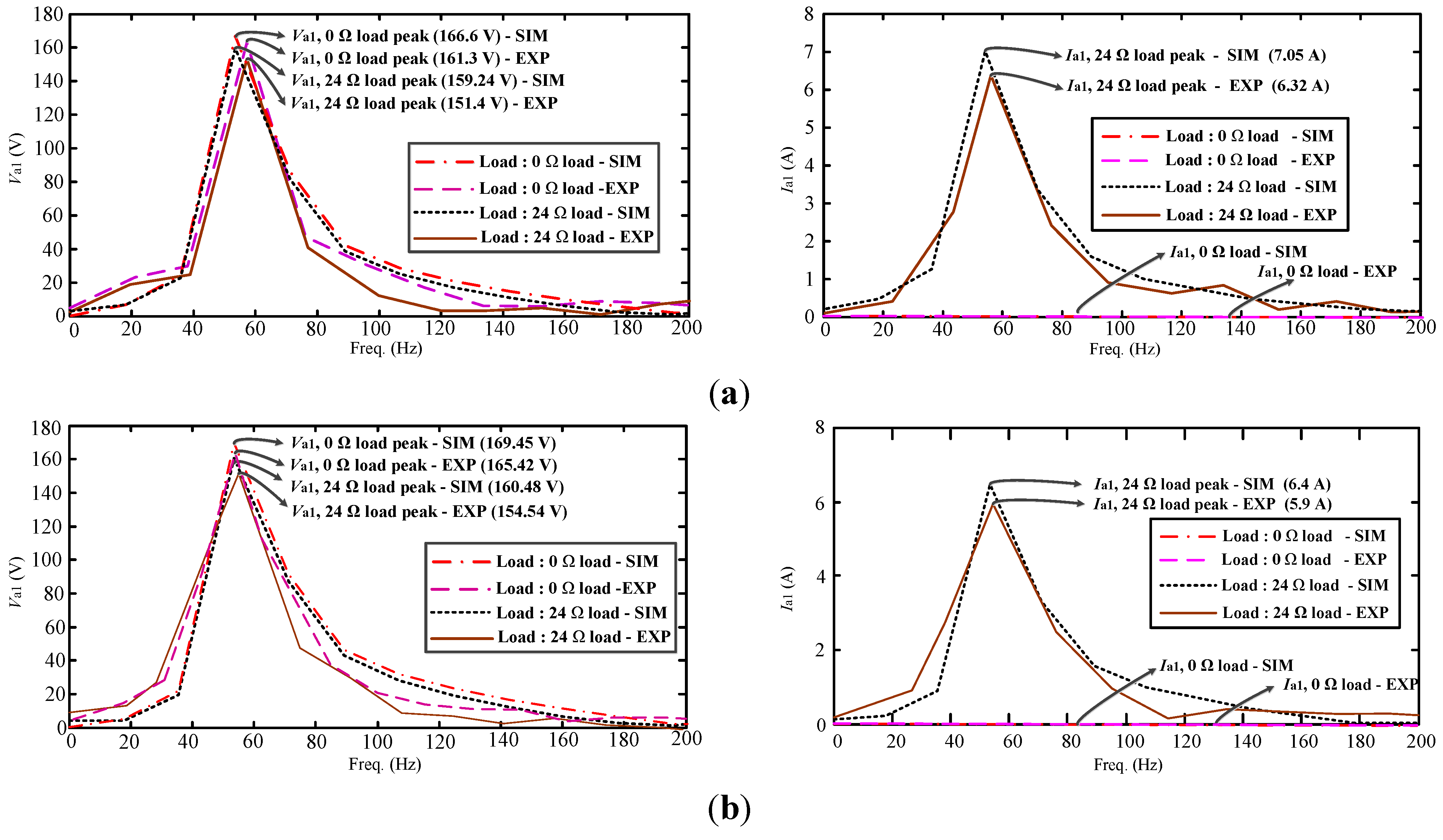
From the frequency domain analysis for
Va
1,
Figure 17 shows that the differences for the peak values of
Va
1 between simulation and experimental results are 7.84 V and 5.94 V for double three-phase winding and six-phase winding, respectively, under 24 Ω load. The corresponding differences for the peak values of
Ia
1 between simulation and experimental results are 0.73 A and 0.50 A.
Figure 17.
Measured induced voltage and current with 24 Ω load: (a) double three-phase winding; (b) six-phase winding.
Figure 17.
Measured induced voltage and current with 24 Ω load: (a) double three-phase winding; (b) six-phase winding.
Finally, a load cell installed at the bottom of the generator will yield torques which, in turn, is used to calculate the input and output powers of the generator for the two winding connections. The results are shown in
Table 9, which indicates that the output powers of 5.029 and 5.433 kW at 90 rpm for 24 Ω load are obtained with efficiencies of 96.56% and 98.54%, respectively, for double three-phase and six-phase winding.
Table 9.
Calculated efficiencies from measured results (Prime mover measured). Vl,rms: the rms of line induced voltage; Il,rms: the rms of line current; ωm: speed; T: torque; Po: output power; Pi: input power; η: efficiency.
Table 9.
Calculated efficiencies from measured results (Prime mover measured). Vl,rms: the rms of line induced voltage; Il,rms: the rms of line current; ωm: speed; T: torque; Po: output power; Pi: input power; η: efficiency.
| Vl,rms (V) | Il,rms (A) | ωm (rpm) | T (kg·m) | Po (W) | Pi (W) | η (%) |
|---|
| Double three-phase winding | 110 | 2.7 | 40 | 27.10 | 1028.84 | 1112.46 | 92.48 |
| 136 | 3.4 | 50 | 33.30 | 1601.80 | 1708.71 | 93.74 |
| 164 | 4.0 | 60 | 39.00 | 2272.45 | 2401.43 | 94.63 |
| 190 | 4.7 | 70 | 45.20 | 3093.44 | 3247.07 | 95.27 |
| 217 | 5.3 | 80 | 50.60 | 3984.06 | 4154.27 | 95.90 |
| 242 | 6.0 | 90 | 56.40 | 5029.88 | 5209.26 | 96.56 |
| Six-phase winding | 115 | 2.8 | 40 | 28.00 | 1115.44 | 1149.40 | 97.05 |
| 144 | 3.5 | 50 | 34.80 | 1745.91 | 1785.68 | 97.77 |
| 171 | 4.2 | 60 | 41.20 | 2487.92 | 2536.90 | 98.07 |
| 198 | 4.9 | 70 | 47.60 | 3360.87 | 3419.48 | 98.29 |
| 226 | 5.5 | 80 | 53.30 | 4305.88 | 4375.95 | 98.40 |
| 253 | 6.2 | 90 | 59.70 | 5433.79 | 5514.06 | 98.54 |
Table 10 compares the aforementioned experimental result from 24 Ω-load with that from Maxwell-2D simulation. It is seen from
Table 10 that close agreement between measured and simulated results are also obtained concerning the induced voltages, load currents and output powers.
Table 10.
Comprehensive comparison.
Table 10.
Comprehensive comparison.
| Winding connection | Maxwell-2D software | Oscilloscope measured | Prime mover measured |
|---|
| No Load | Load 24 Ω | No Load | Load 24 Ω | No Load | Load 24 Ω |
|---|
| Vp (V) | Ip (A) | Vp (V) | Ip (A) | Po (W) | Vp (V) | Ip (A) | Vp (V) | Ip (A) | Po (W) | Vp (V) | Ip (A) | Vp (V) | Ip (A) | Po (W) |
|---|
| Double three-phase winding | 208 | 0.0 | 199 | 8.3 | 4955 | 209 | 0.0 | 200 | 8.1 | 4860 | 212 | 0.0 | 198 | 8.5 | 5030 |
| Six-phase winding | 215 | 0.0 | 204 | 8.5 | 5315 | 217 | 0.0 | 204 | 8.3 | 5080 | 222 | 0.0 | 207 | 8.8 | 5434 |


