Exploring the Potential for Increased Production from the Wave Energy Converter Lifesaver by Reactive Control

Abstract
:1. Introduction
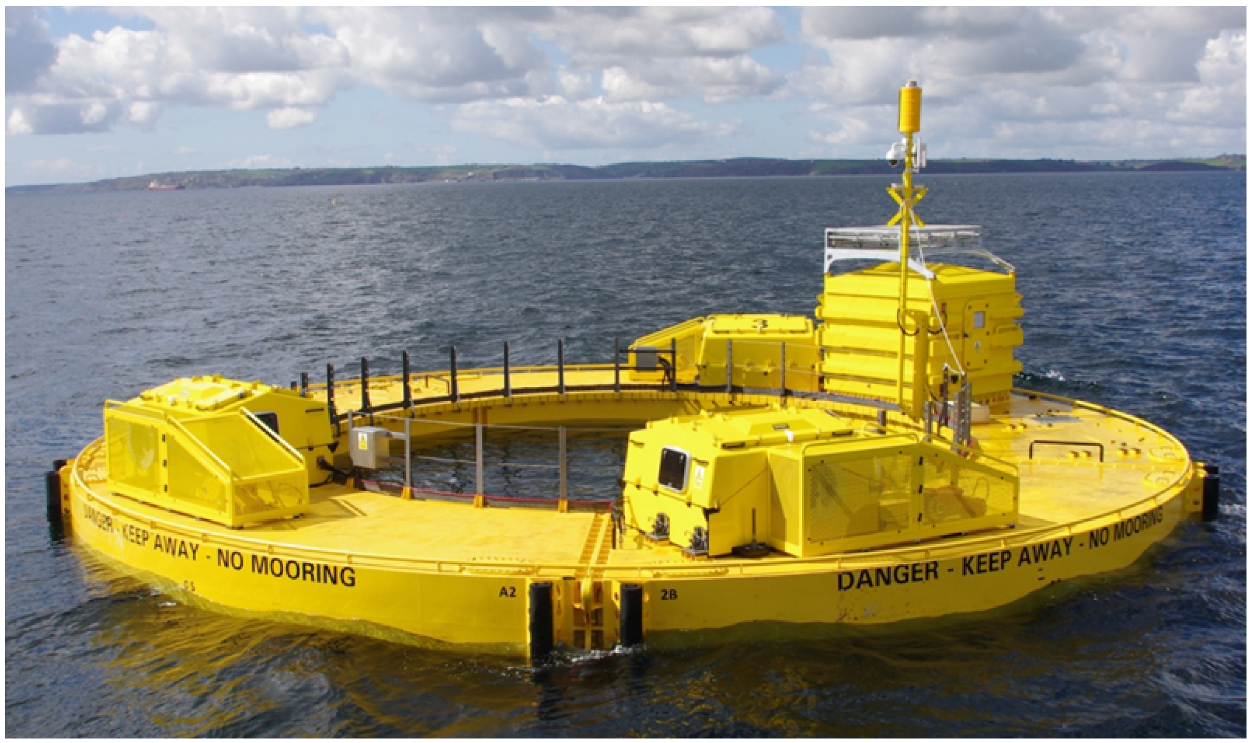
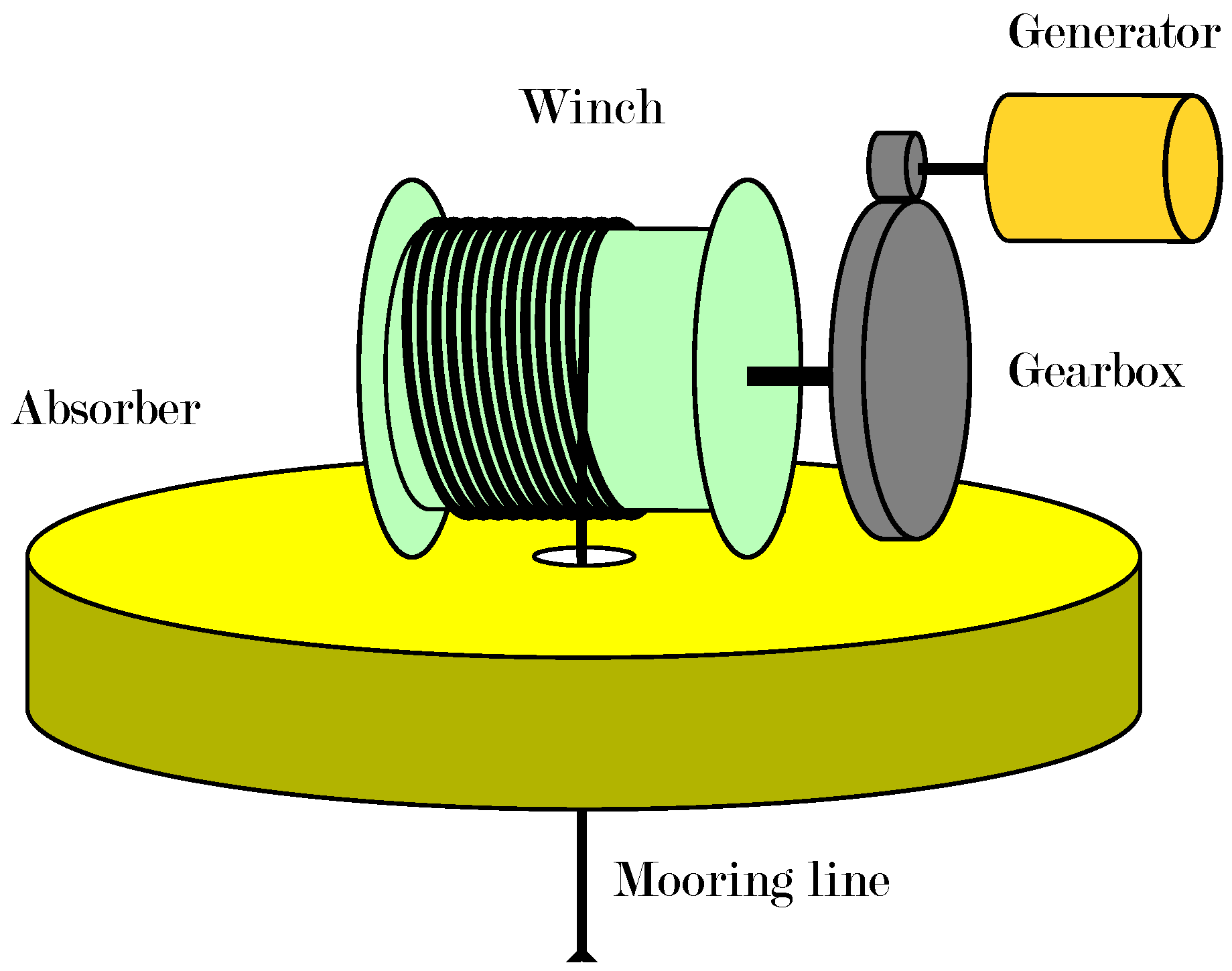
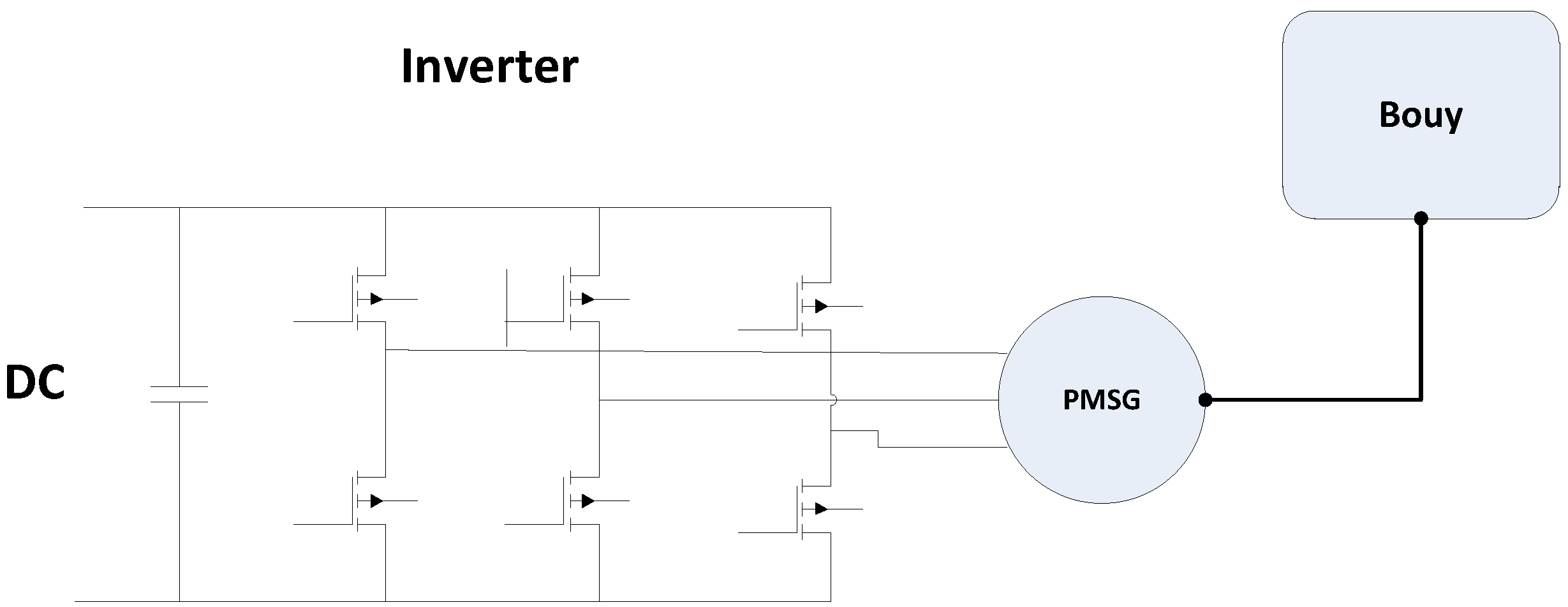
1.1. Description of the Investigated System
2. Hydrodynamic Model
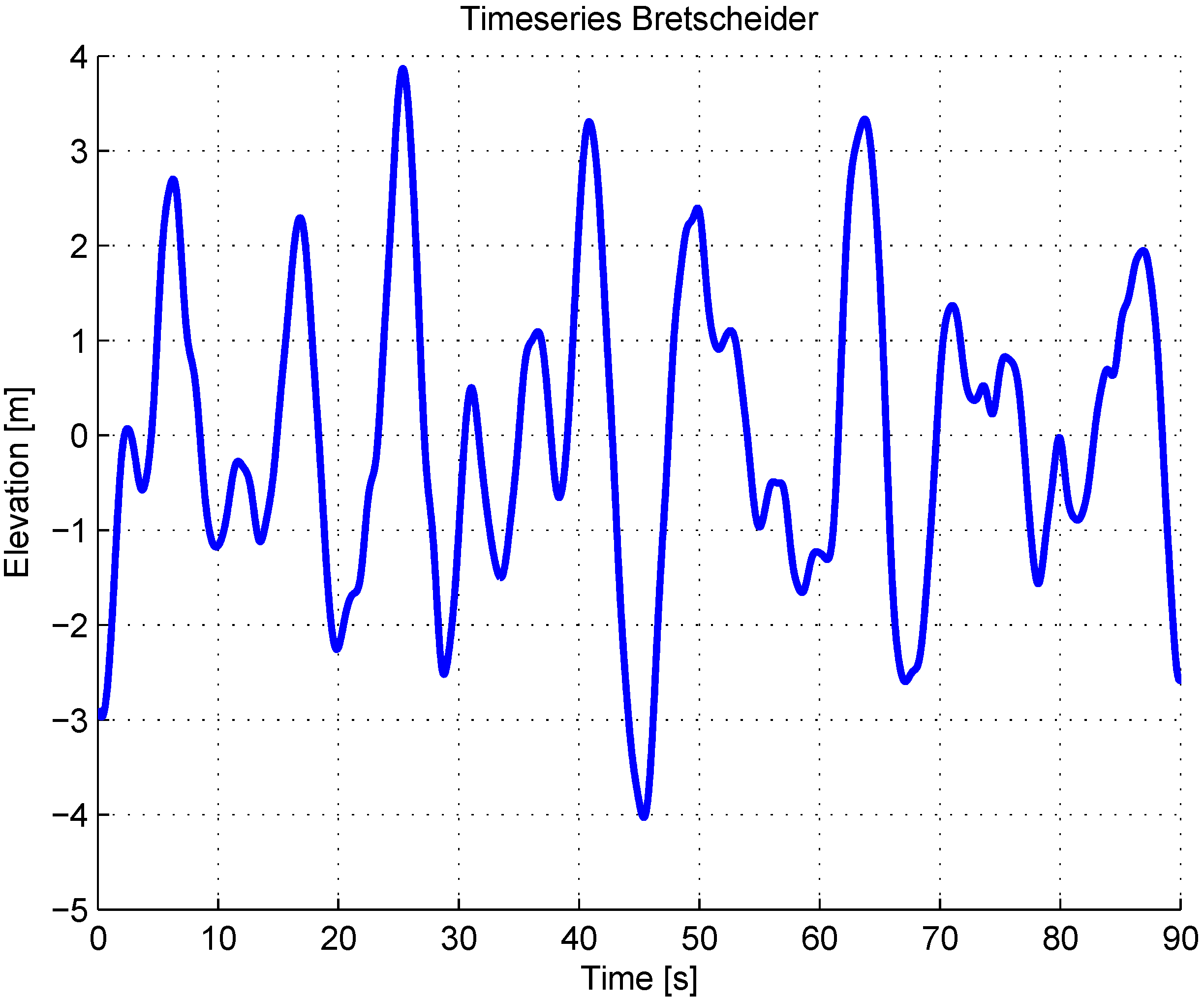
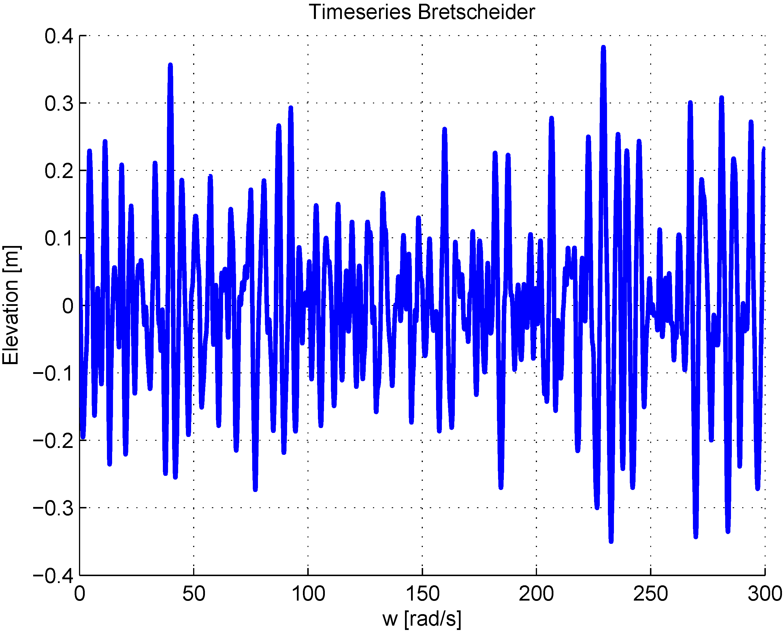
- Wave elevation time-series;
- Load force, , given by the load force parameters, damping, , and added mass, .
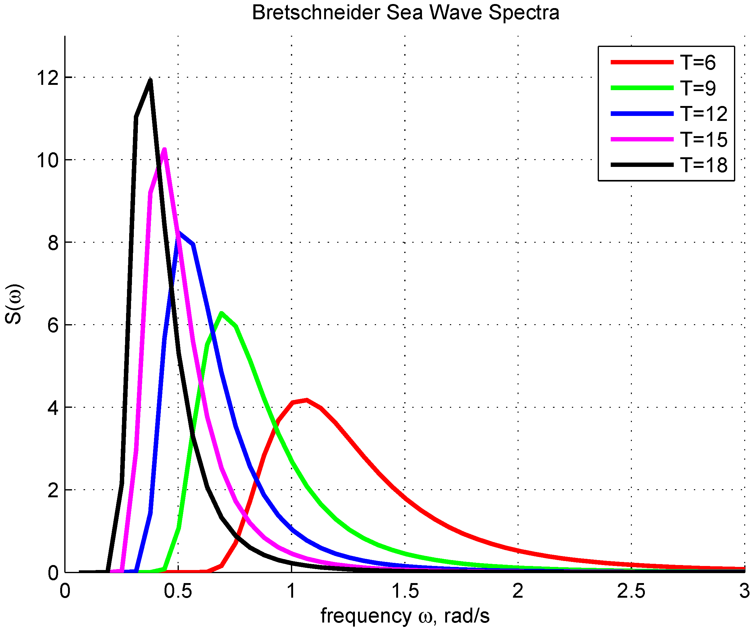
2.1. Generation of Wave Elevation Time Series
2.2. Forces Acting on the WEC System
2.2.1. Hydrostatic Force
2.2.2. Radiation Force
2.2.3. Excitation Force
2.2.4. Load Force
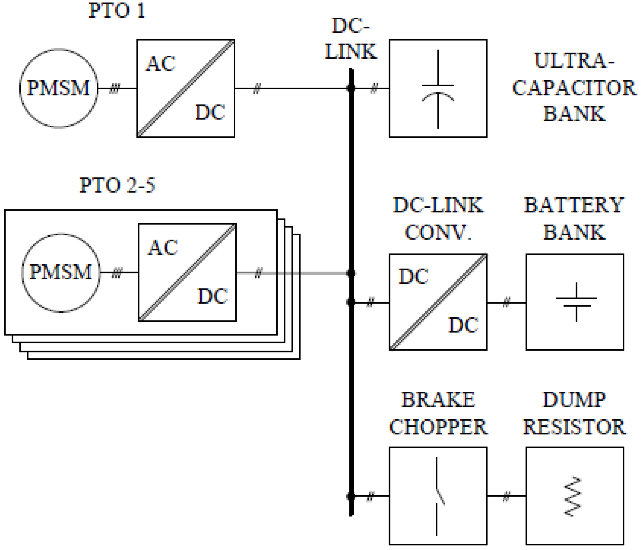
3. Electric Power Take-off System
- Permanent Magnet Synchronous Machine;
- Inverter/Rectifiers;
- Ultra-capacitor Bank;
- DC-link Charger;
- Battery Charger;
- Brake Charger and Dump Resistor.


| Property | Value | Unit |
|---|---|---|
| Generator nominal speed | 400 | rpm |
| Generator maximum torque | 3700 | Nm |
| DC-bus voltage | 600 | V |
| Angular to linear gear ratio | 38.5 | 1/m |
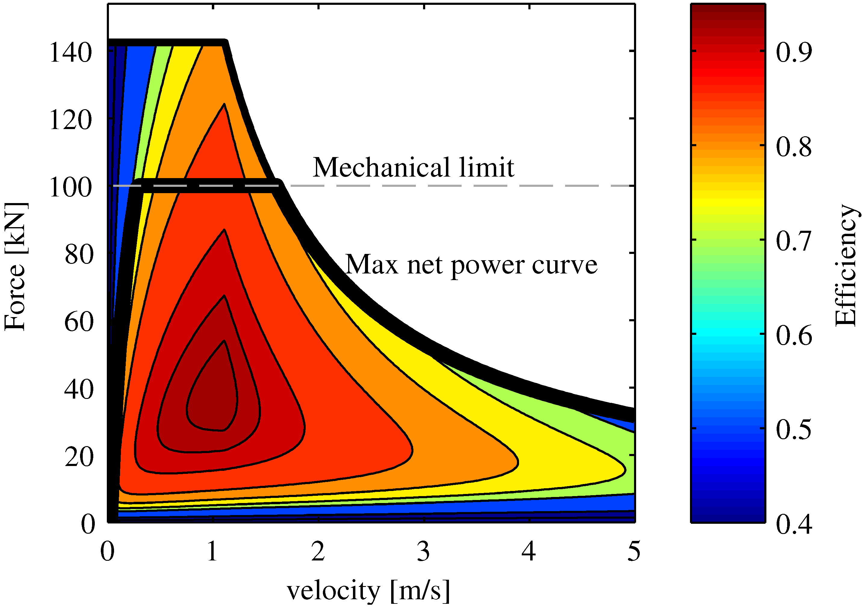
| PTO maximum force | 100 | kN |
| PTO minimum force | 10 | kN |
| PTO nominal speed | 1.1 | m/s |
3.1. PWM Converter Modeling
- Simulation time is significantly reduced. Even for low switching frequencies in the converter bridge, the simulation time becomes tenfold times longer than with the unity block solution;
- No filter is needed in the system in order to evaluate voltage measurements, as the harmonic distortion due to the high frequency switching is not present.
3.2. Modeling and Control of the Permanent Magnet Synchronous Generator
| Property | Value | Unit |
|---|---|---|
| Rated Power, | 83.7 | kW |
| Rated Voltage, | 400 | V |
| Number of poles, | 28 | |
| Torque constant, | 10.8 | Nm/A |
| Winding resistance, | 0.038 | Ω |
| Inductance, L | 1.4 | mH |
| Inertia, | 1.31 | kg |
| Permanent magnet flux, | 0.257 | Wb |
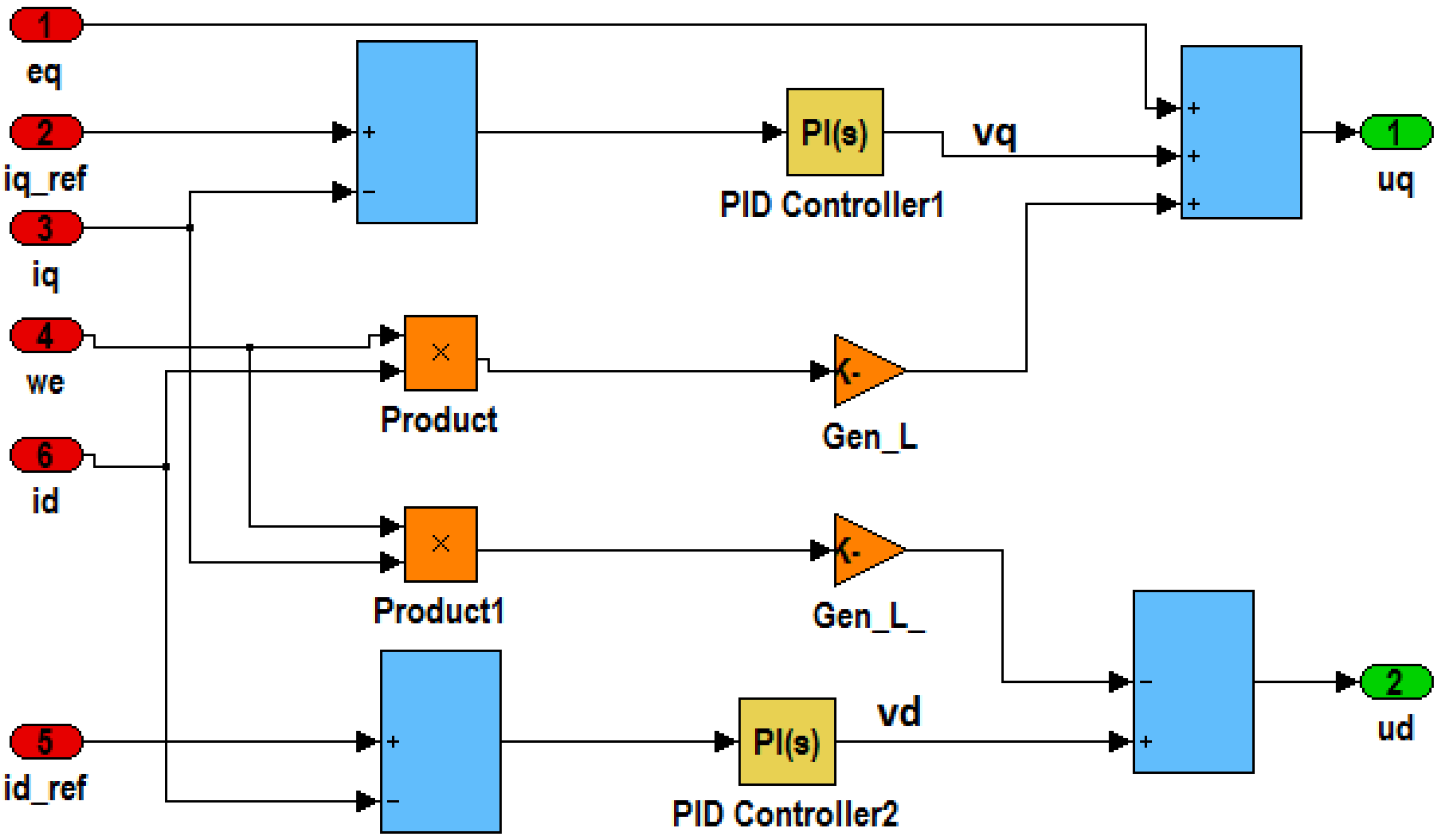
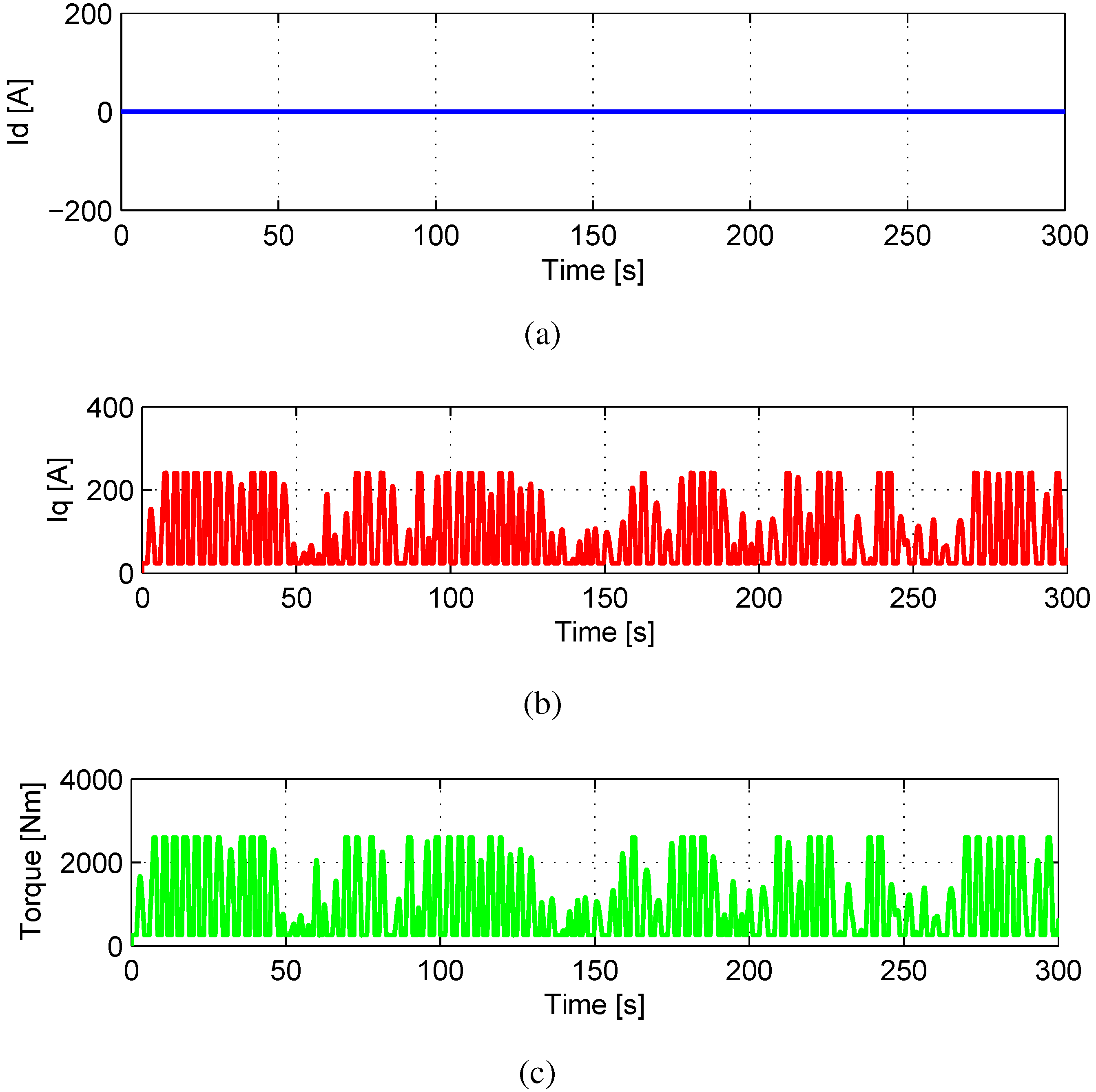
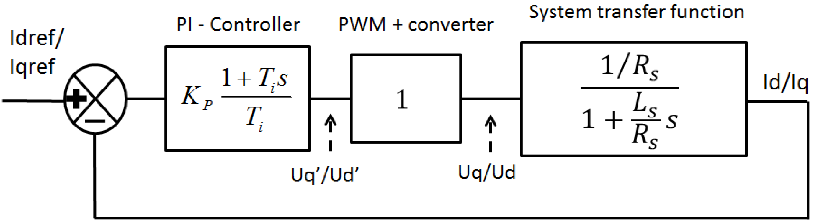
3.2.1. Current Control

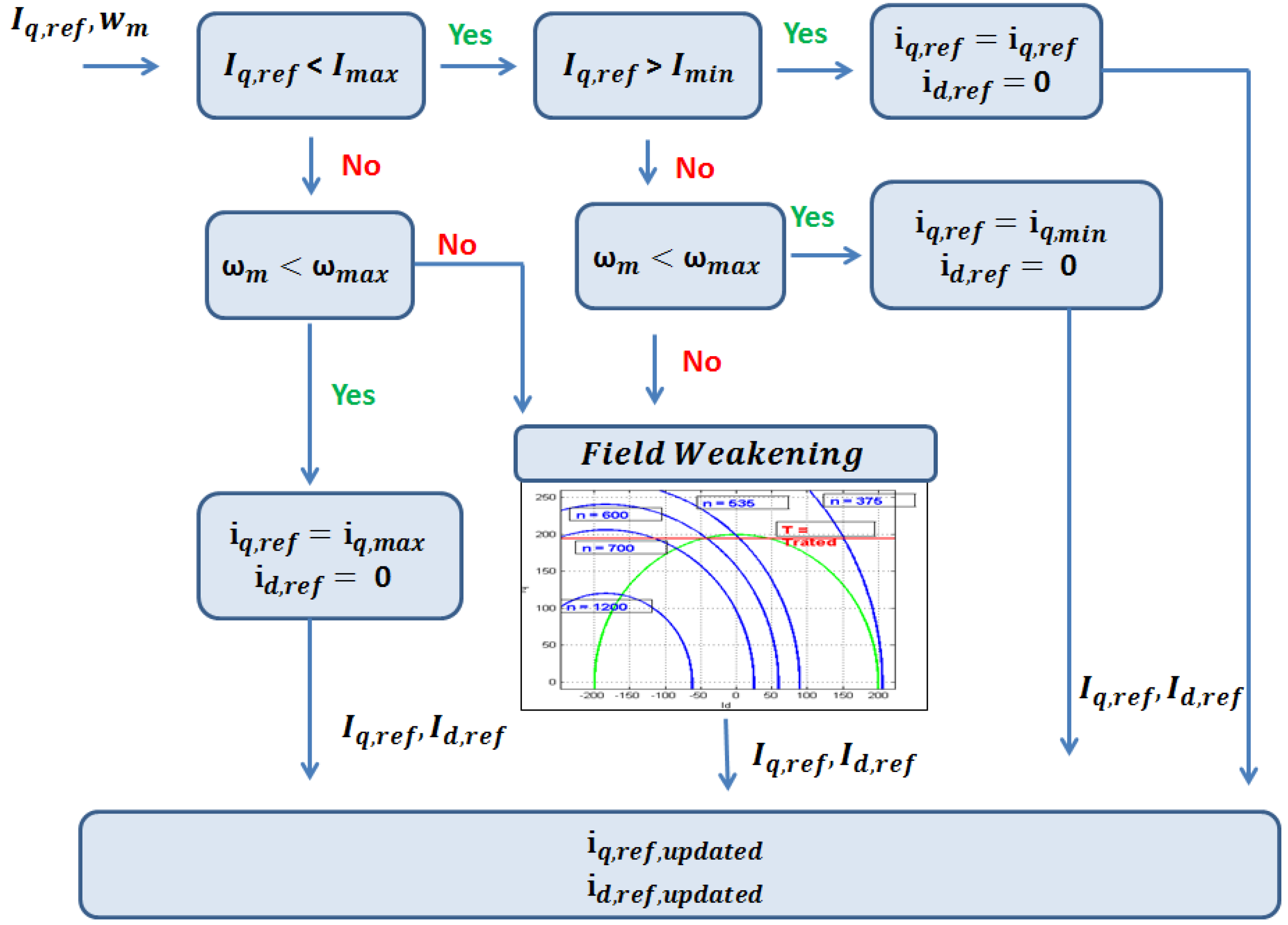
3.2.2. Torque Control

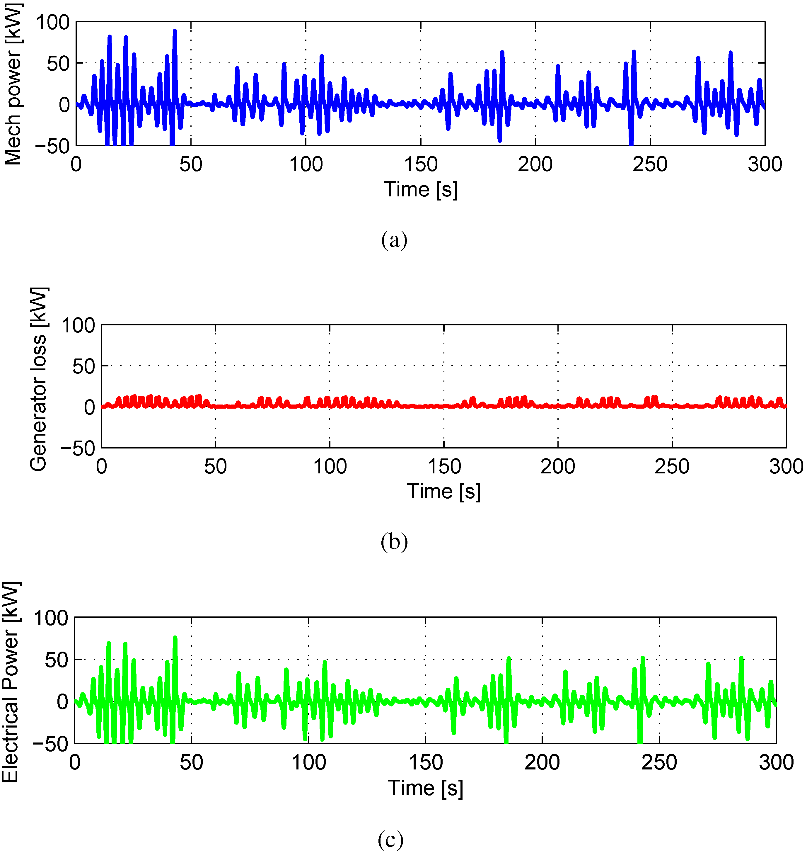
3.3. Generator Efficiency

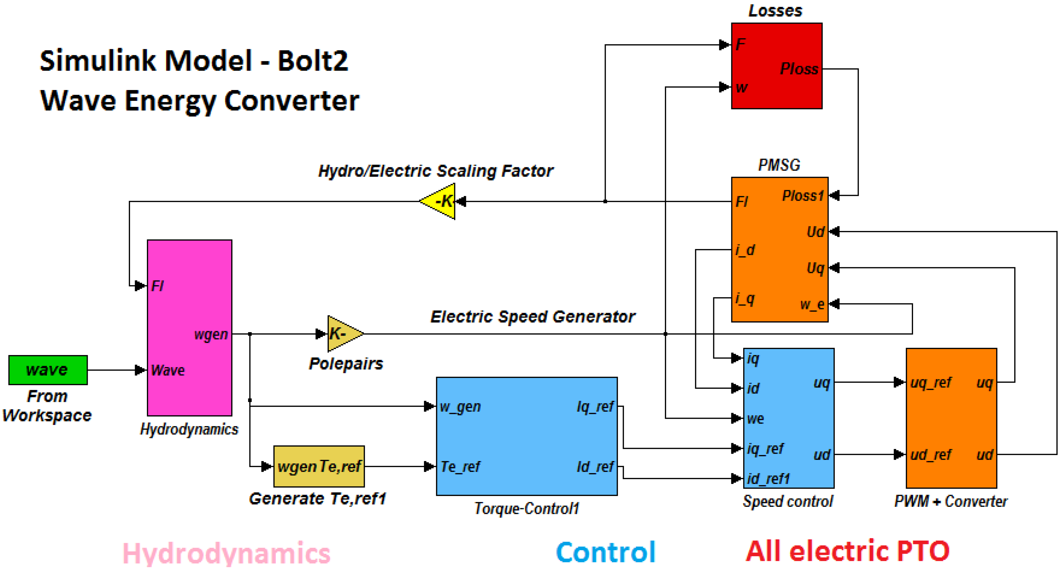
4. Wave-to-Wire Modeling
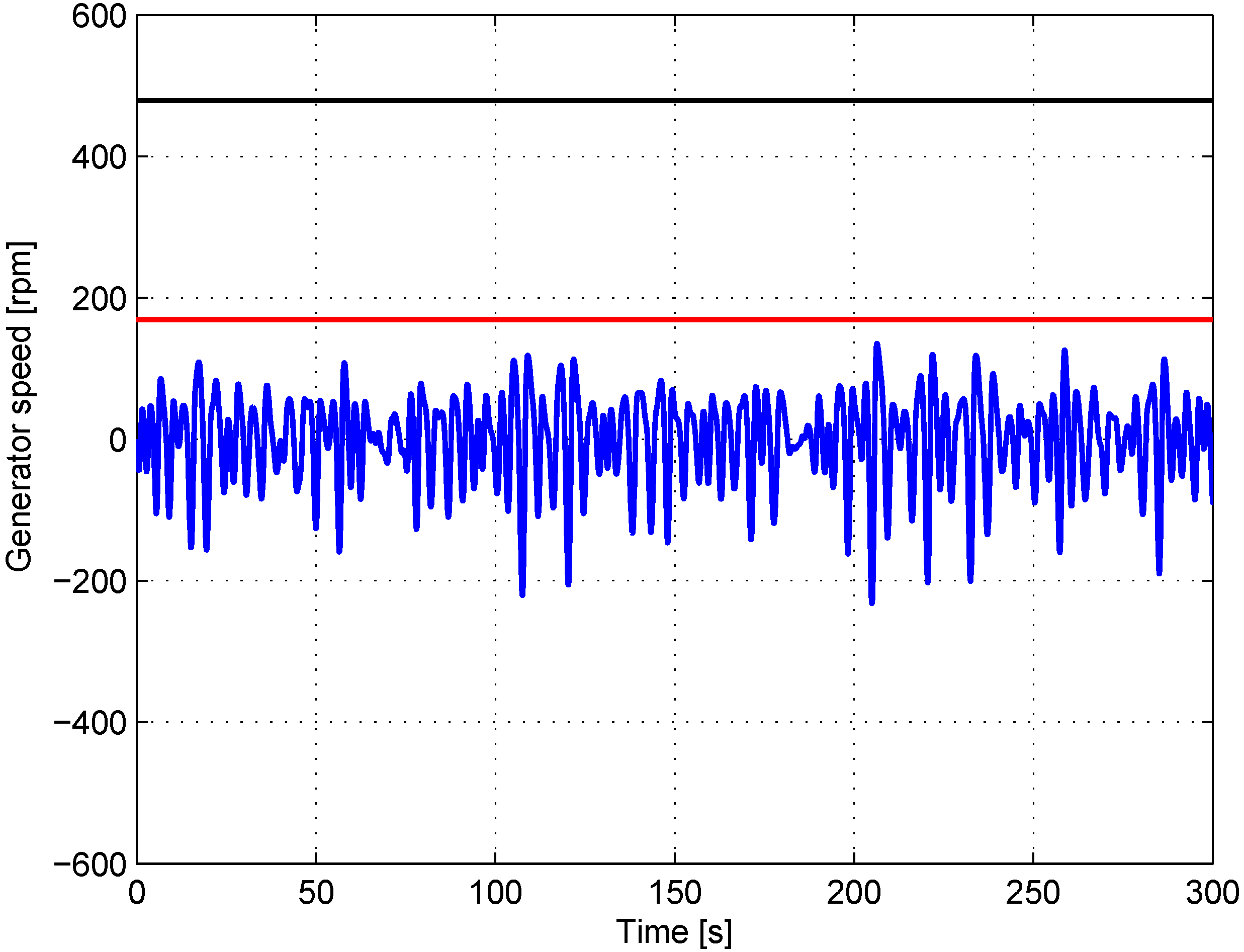
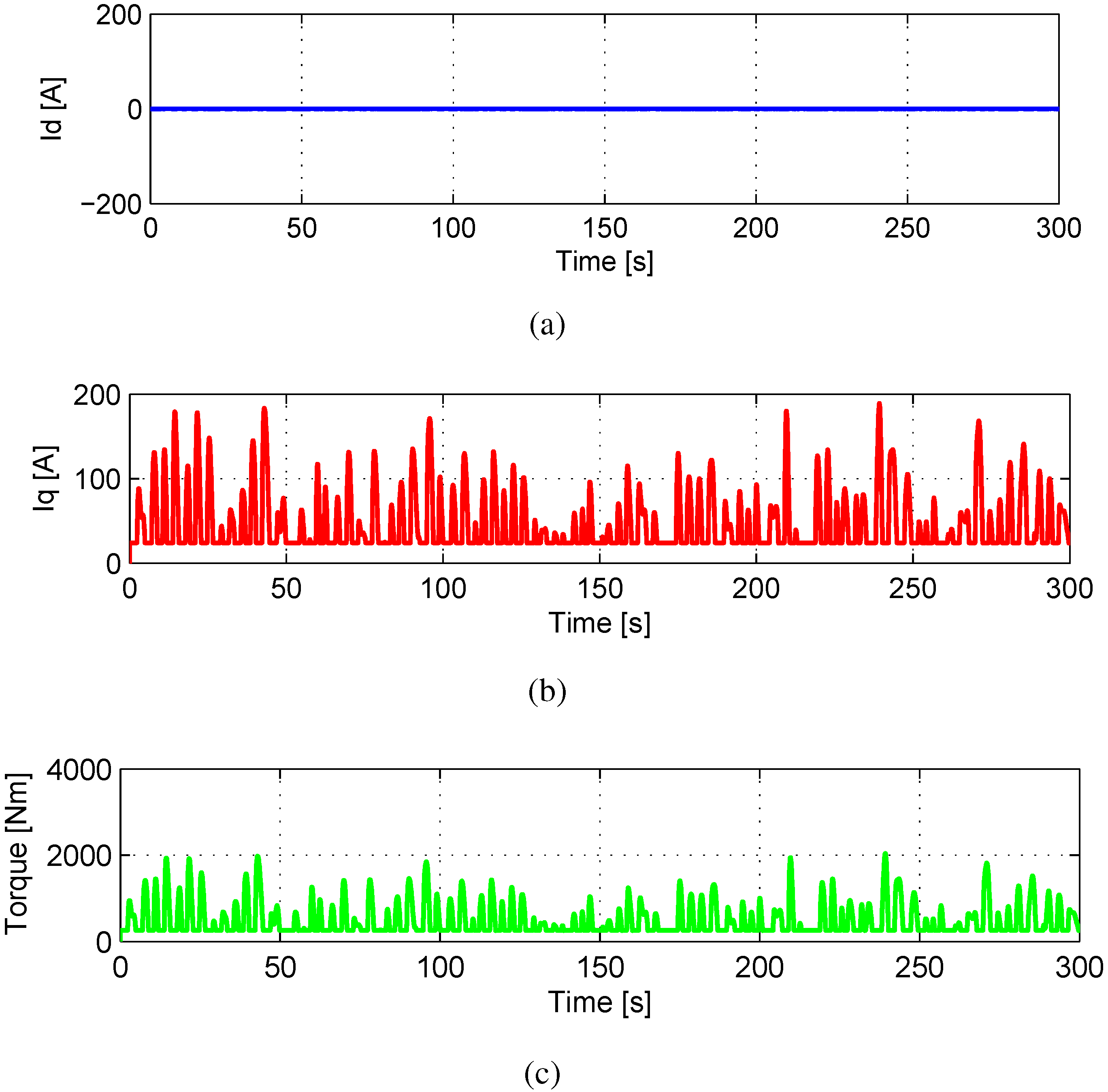
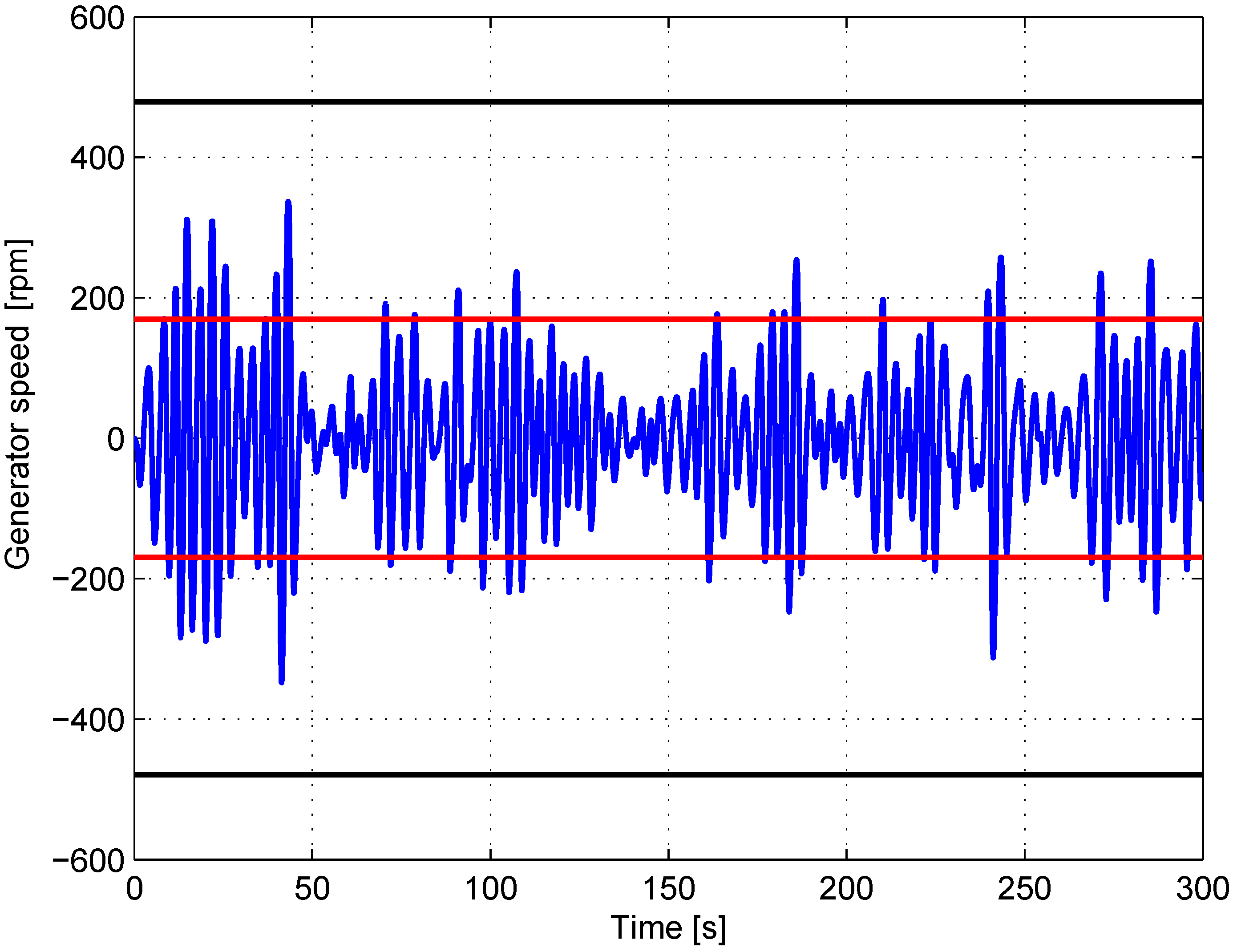
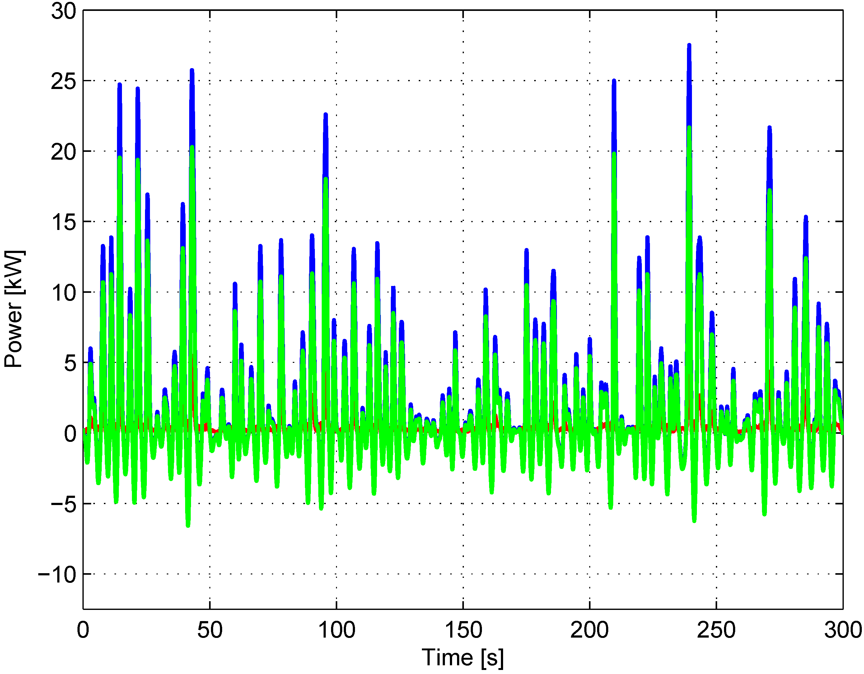
4.1. Simulation Results for a Passive Loaded System


4.2. Simulation Results for a Reactive Controlled System

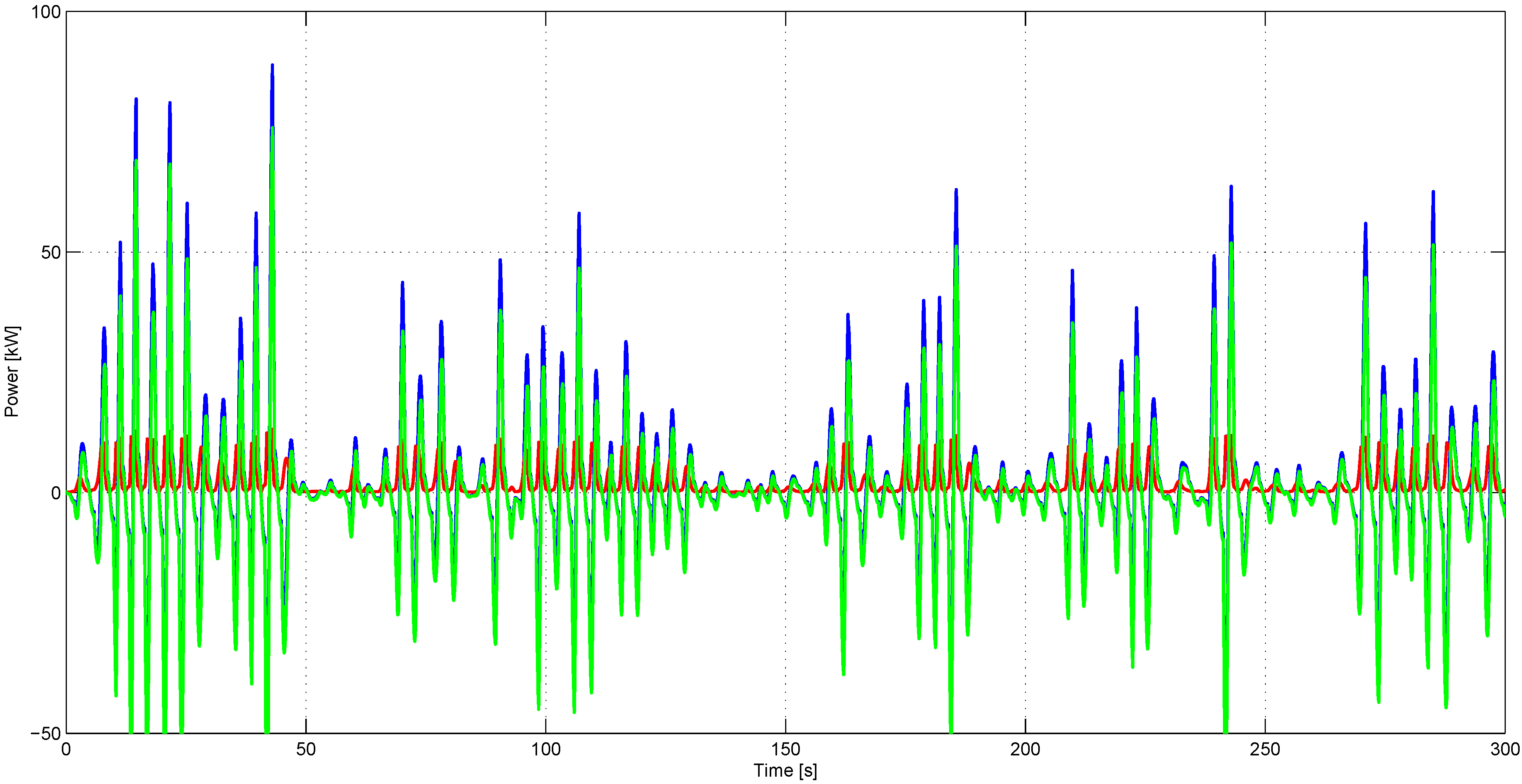
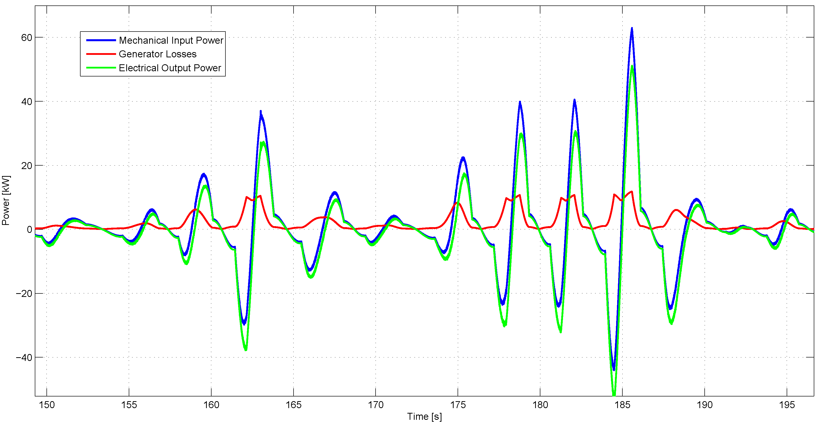
4.2.1. Performance of Passive Loading vs. Reactive Control
- Approximate complex conjugate control leads to increased mechanical power extraction;
- However, the generator efficiency becomes more important, as the bi-directional power peaks both contribute to the average losses;
- As Lifesaver has an average generator efficiency of around 80% in the design wave state and lower efficiency in the lower wave states, the losses can become very large;
- Due to this, approximate complex conjugate control does not give maximum electrical power output.
4.3. Maximizing Electrical Output Power-Table for Sub-Optimal Operation Parameters
4.3.1. Example Identification of Optimal Control Parameters for a Low Wave State


4.3.2. Observations from Mapping of Control Parameters
- Combining the maps of output mechanical power and generator losses, a map of optimal control parameters with respect to electrical output power is made;
- For sea states with low significant wave height, the optimal control parameters have a larger component of added mass and smaller component of added damping;
- For the sea states with low significant height, the average power is increased by a significant factor, i.e., 10% for ;
- When the significant wave height increases, the optimal control parameters shift towards a larger factor of added damping;
- For the sea states with a higher significant wave height, the increase in average power compared with the reference case of passive loading goes towards zero;
- For a sea state with lower peak periods, the optimal control parameters have a larger damping factor;
- For increasing peak periods, the optimal control parameters have larger fraction of added damping. This means that the optimal control moves towards complex conjugate control;
4.4. Energy Calculations-Potential Increase in Annual Energy Production with Optimal Control
- and are the sea states that represents the low energy sea states;
- and represent the medium energy sea states;
- and represent the high energy sea states.

| Low energy | Medium energy | High energy | Total | |
|---|---|---|---|---|
| Hours per wave state | 2182 | 4370 | 2468 | 8760 |
| Av. Pow. Pass. (kW) | 6.70 | 19.04 | 31.40 | - |
| Av. Pow. Opt. (kW) | 7.02 | 19.24 | 31.47 | - |
| Diff (%) | 4.78 | 1.4 | 0.22 | - |
| Ener. Pass. (MWh) | 14.62 | 83.22 | 77.53 | 175.37 |
| Ener. Opt. (MWh) | 15.32 | 84.10 | 77.70 | 177.12 |
| Difference (%) | 4.78 | 1.40 | 0.22 | 1.0 |
5. Discussion
- A full wave-to-wire model of Lifesaver point absorber with all-electric power take off system has been made in Matlab and Simulink;
- The main characteristics of the Lifesaver generator and power take off system have been modeled using classical representation of a Permanent Magnet Synchronous Machine complete with field weakening operation and a simplified model of the inverter and DC-link;
- A control method has been demonstrated that enforces the force, voltages and currents within the different rating constraints of the power take-off system, even for the sea states with high significant wave height;
- Wave-to-wire simulations show that Lifesaver has limited potential for increased power extraction using reactive control, due to the force and efficiency limitations of the generator; Analysis shows that the if the device is optimally controlled, only a 1% increase in annual energy production can be expected compared to the reference case of passive loading.
5.1. Aspects of Practical Implementation in Lifesaver
- Hydrodynamic model of Lifesaver is not completely accurate;
- The validity and accuracy of the simplified PMSM model used;
- The damping coefficients used by Lifesaver in the sea are not the same found to give optimal power extraction in the model.
5.2. Implications for a Generic WEC
6. Conclusions
Acknowledgments
References
- Thorpe, T. 2010 Survey of Energy Resources; Technical Report for World Energy Council: London, UK, 2010. [Google Scholar]
- International Energy Agency (IEA). Electricity in the World; Technical Report; IEA: Paris, France, 2008. [Google Scholar]
- Wave Hub. Available online: http://www.wavehub.co.uk (accessed on 12 July 2013).
- Falnes, J. Ocean Waves and Oscillating Systems, Linear Interaction Including Wave-Energy Extraction; Cambridge University Press: Cambridge, UK, 2002. [Google Scholar]
- Falnes, J. Principles for Capturie of Energy from Ocean Waves: Phase Control and Optimum Oscillation; Technical Report for Norwegian University of Science and Technology: Trondheim, Norway, 1997; Available online: http://folk.ntnu.no/falnes/w_e/index.html (accessed on 12 July 2013).
- Falnes, J.; Hals, J. Heaving buoys, point absorbers and arrays. Philos. Trans. R. Soc. A Math. Phys. Eng. Sci. 2012, 370, 246–277. [Google Scholar] [CrossRef] [PubMed]
- Falnes, J.; Lillebrekken, P.M. Budal’s Latching-Controlled-Buoy Type Wave-Power Plant. In Proceedings of the 5th European Wave Energy Conference, Cork, Ireland, 17–20 September 2003.
- Hals, J. Modelling and Phase Control of Wave-Energy Converters. Ph.D. Thesis, Norwegian University of Science and Technology, Trondheim, Norway, 2010. [Google Scholar]
- Tedeschi, E.; Molinas, M. Tunable control strategy for wave energy converters with limited power takeoff rating. IEEE Trans. Ind. Electron. 2012, 59, 3838–3846. [Google Scholar] [CrossRef]
- Sandvik, C.; Molinas, M.; Sjolte, J. Time Domain Modelling of the Wave-to-Wire Energy Convert Bolt. In Proceedings of the 7th International Conference and Exhibition on Ecological Vehicles and Renewable Energies, Monte Carlo, Monaco, 22–25 March 2012.
- Mitchell, W.H. Sea spectra revisited. Mar. Technol. 1999, 4, 211–227. [Google Scholar]
- Dean, R.; Dalrymple, R. Water Wave Mechanics for Engineers and Scientists; Prentice Hall: Upper Saddle River, NJ, USA, 1984. [Google Scholar]
- Newman, J. Marine Hydrodynamics; Mit Press: Cambridge, MA, USA, 1977. [Google Scholar]
- Cummins, W.E. The Impulse Response Functions and Ship Motions; Department of the Navy, David Taylor Model Basin: Bethesda, MD, USA, 1962. [Google Scholar]
- Taghipour, R.; Perez, T.; Moan, T. Hybrid frequencytime domain models for dynamic response analysis of marine structures. Ocean Eng. 2008, 35, 685–705. [Google Scholar] [CrossRef]
- Kung, S. A New Identification and Model Reduction Algorithm via Singular Value Decompositions. In Proceedings of the 12th Aslilomar Conference on Circuits, Systems and Computers, Pacific Grove, CA, USA, 6–8 November 1978; pp. 705–714.
- Mohan, N. Advanced Electric Drives Analysis, Control and Modeling Using Simulink; Minnesota Power Electronics Research & Education (MNPERE): Minneapolis MN, USA, 2001. [Google Scholar]
- Umland, J.; Safiuddin, M. Magnitude and Symmetric Optimum Criterion for the Design of Linear Control Systems—What Is It and Does It Compare with the others? In Proceedings of the IEEE Industry Applications Society Annual Meeting, Salt Lake City, UT, USA, 2–7 October 1988; pp. 1796–1802.
- Pan, C.T.; Liaw, J.H. A robust field-weakening control strategy for surface-mounted permanent-magnet motor drives. IEEE Trans. Energy Conver. 2005, 20, 701–709. [Google Scholar] [CrossRef]
- Tedeschi, E.; Molinas, M.; Carraro, M.; Mattavelli, P. Analysis of Power Extraction from Irregular Waves by All-Electric Power Take off. In Proceedings of the IEEE Energy Conversion Congress and Exposition (ECCE), Phoenix, AZ, USA, 12–16 September 2010; pp. 2370–2377.
- Sjolte, J.; Bjerke, I.; Hjetland, E.; Tjensvoll, G. All-Electric Wave Energy Power Take off Generator Optimized by High Overspeed. In Proceedings of the Submitted to the European Wave and Tidal Energy Conference (EWTEC11), Southampton, UK, 5–9 September 2011.
- Molinas, M.; Skjervheim, O.; Sørby, B.; Andreasen, P.; Lundberg, S.; Undeland, T. Power Smoothing by Aggregation of Wave Energy Converters for Minimizing Electrical Energy Storage Requirements. In Proceedings of the Submitted to the European Wave and Tidal Energy Conference (EWTEC07), Porto, Portugal, 11–13 September 2007.
- Sjolte, J.; Tjensvoll, G.; Molinas, M. All-Electric Wave Energy Converter Array with Energy Storage and Reactive Power Compensation for Improved Power Quality. In Proceedings of the IEEE Energy Conversion Congress and Exposition (ECCE), Raleigh, NC, USA, 15–20 September 2012; pp. 954–961.
- Tedeschi, E.; Molinas, M. Impact of Control Strategies on the Rating of Electric Power Take off for Wave Energy Conversion. In Proceedings of the IEEE International Symposium on Industrial Electronics, Bari, Italy, 4–7 July 2010; pp. 2406–2411.
© 2013 by the authors; licensee MDPI, Basel, Switzerland. This article is an open access article distributed under the terms and conditions of the Creative Commons Attribution license ( http://creativecommons.org/licenses/by/3.0/).
Share and Cite
Sjolte, J.; Sandvik, C.M.; Tedeschi, E.; Molinas, M. Exploring the Potential for Increased Production from the Wave Energy Converter Lifesaver by Reactive Control. Energies 2013, 6, 3706-3733. https://doi.org/10.3390/en6083706
Sjolte J, Sandvik CM, Tedeschi E, Molinas M. Exploring the Potential for Increased Production from the Wave Energy Converter Lifesaver by Reactive Control. Energies. 2013; 6(8):3706-3733. https://doi.org/10.3390/en6083706
Chicago/Turabian StyleSjolte, Jonas, Christian McLisky Sandvik, Elisabetta Tedeschi, and Marta Molinas. 2013. "Exploring the Potential for Increased Production from the Wave Energy Converter Lifesaver by Reactive Control" Energies 6, no. 8: 3706-3733. https://doi.org/10.3390/en6083706