1. Introduction
Energy is an important aspect of daily life and ongoing human development [
1]. Owing to the associated complexities and uncertainties [
2,
3,
4], decision makers and planners are facing increased pressure to respond more effectively to a number of energy-related issues and conflicts, including conservation voltage reduction (CVR), which is a reduction in energy consumption resulting from a reduction in feeder voltage [
5]. Although CVR leads to out-of-range voltages for some customers [
6], it is widely used on account of its two key benefits: peak load reduction and lower annual energy consumption. In Korea, CVR is mainly used for peak load reduction (for example, five times in the summer of 2012 and twelve times in the winter of 2012). To analyze the effects of CVR at a national level, load modeling should first be carried out. Load modeling is the process of defining load characteristics via mathematical formulas that describe the characteristics of load changes in response to voltage and frequency variations. Load modeling techniques can be classified as either component based [
7,
8,
9,
10,
11] or measurement based [
12,
13,
14,
15,
16,
17,
18,
19,
20,
21,
22,
23,
24], depending on the modeling procedure. In component-based load modeling, measuring devices need not be installed in the field. However, this type of procedure is not efficient for describing the characteristics of rapidly changing loads, as each individual load must be analyzed in the laboratory before aggregating the loads. Component-based load modeling might be appropriate for use as a complement to measurement-based load modeling. On the other hand, measurement-based load modeling can accurately reflect load characteristics by direct measurement of the loads. Therefore, most current research on load modeling is focused on measurement-based methods, even though these methods require installation of an additional measuring device for every load in the power system. Measurement-based load modeling can be sub-classified into static load modeling [
12,
13,
14] and dynamic load modeling [
15,
16,
17,
18,
19,
20,
21,
22,
23,
24]. Although dynamic load modeling can reflect the transient characteristics of loads, it requires high-density data samples on the time axis. In contrast, static load modeling requires relatively low-density data samples. In other words, when the measuring devices have low sampling rates, dynamic load modeling cannot be used, and only static load modeling is feasible. In this study, static load modeling was selected based on the realistic constraint that high-performance measuring devices, such as digital fault recorders and power quality meters, may not be installed on every bus in a modern power system.
The purpose of this paper is to propose a static load model for evaluating the effect of conservation voltage reduction at a national level. The model is defined as a linearized load model based on energy management system (EMS) data. The paper is divided into five sections, including this Introduction.
Section 2 describes the formulation of the linearized load model, and
Section 3 presents PSS/E simulation results for the model. In
Section 4, the linearizing parameters for aggregated loads in an actual Korean power system are estimated. Our conclusions are presented in
Section 5.
2. Linearized Load Modeling Based on EMS Data
Load modeling describes the characteristics of numerous intricately connected loads in a relatively brief way. In particular, static load modeling only includes the steady-state characteristics of the loads. ZIP modeling and exponential modeling are representative static load modeling methods. In contrast, dynamic load modeling includes both transient characteristics and steady-state characteristics. State-variable equation modeling and induction-machine modeling are representative dynamic load modeling methods. Because EMS data are usually sampled every few seconds, they do not include the transient characteristics of loads. For example, in Korea, EMS data are sampled every 4 s. Therefore, it is not appropriate to use EMS data to estimate the parameters of dynamic load modeling. On the other hand, the parameters of static load modeling can be estimated using EMS data because only steady-state characteristics are required for static load modeling. In particular, ZIP modeling has a simple structure, and its parameters can be estimated with only a few data samples. Moreover, since ZIP modeling can represent the physical meaning of loads and it is used by many electrical companies to operate their power systems, it is one of the most appropriate modeling techniques for estimating parameters based on the EMS data. In ZIP modeling, a load is composed of constant impedance (
Z), constant current (
I), and constant power (
P) elements. Assuming that
k denotes the
kth conservation voltage reduction, the active power consumption of a load is given by:
where:
;
: Active power consumption of the load before the kth conservation voltage reduction;
: Active power consumption of the load after the kth conservation voltage reduction;
: Terminal voltage before the kth conservation voltage reduction;
: Terminal voltage after the kth conservation voltage reduction;
: Constant impedance fraction of the active power consumption;
: Constant current fraction of the active power consumption;
: Constant power fraction of the active power consumption.
Similarly, the reactive power consumption of a load is given by:
where:
;
: Reactive power consumption of the load before the kth conservation voltage reduction;
: Reactive power consumption of the load after the kth conservation voltage reduction;
: Constant impedance fraction of the reactive power consumption;
: Constant current fraction of the reactive power consumption;
: Constant power fraction of the reactive power consumption.
For the sake of consistency, Equations (1) and (2) can be normalized as:
where:
: Normalized active power consumption;
: Normalized reactive power consumption;
: Normalized terminal voltage.
Given that the values of , , and can be obtained from EMS data, the active ZIP parameters (, , ) and the reactive ZIP parameters (, , ) are to be estimated.
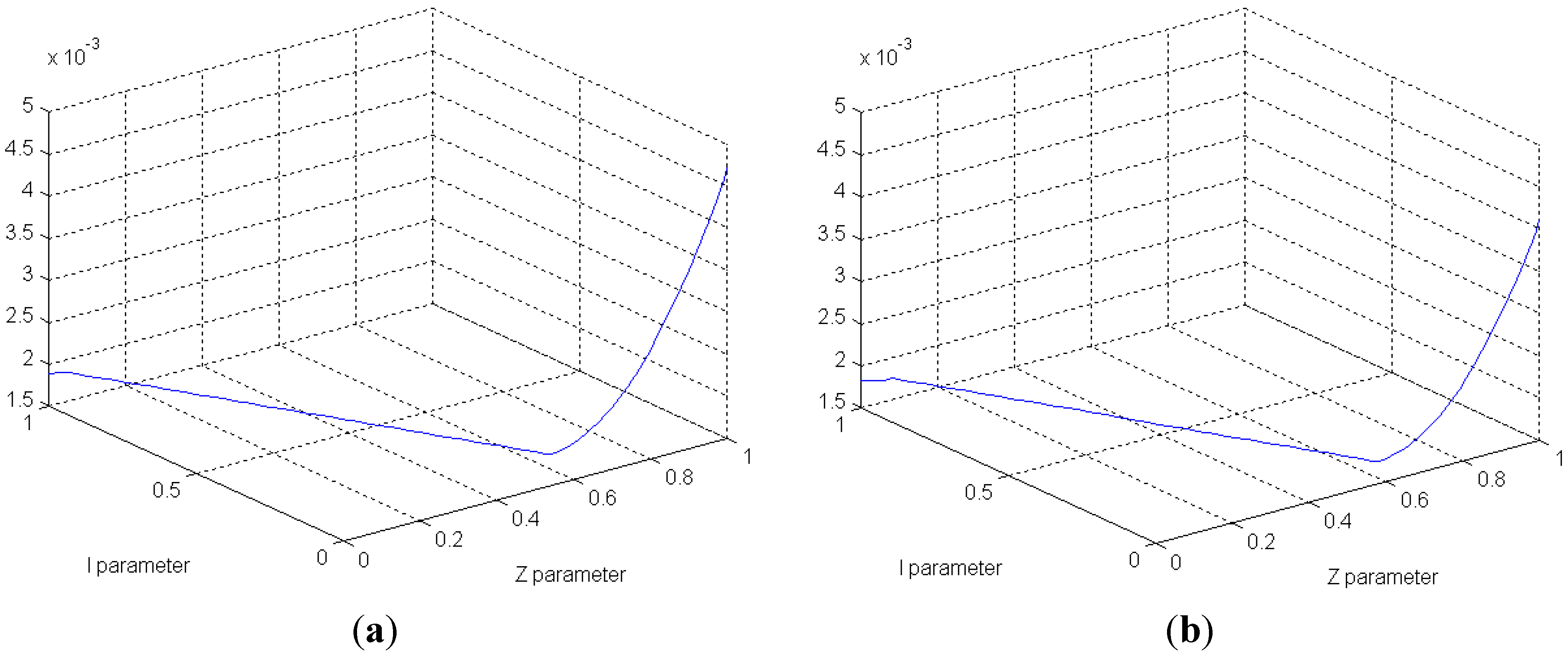
To estimate the active ZIP parameters, the active objective function is defined as:
subject to:
;
,
,
.
If
denotes the voltage variation due to the
kth conservation voltage reduction, Equation (3) can be modified to:
This can be rearranged as follows:
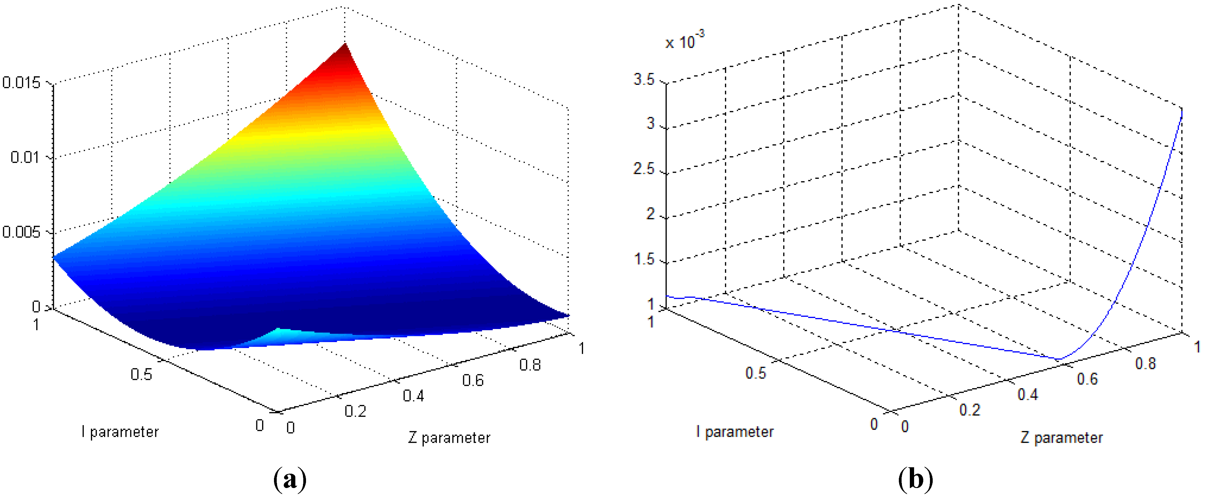
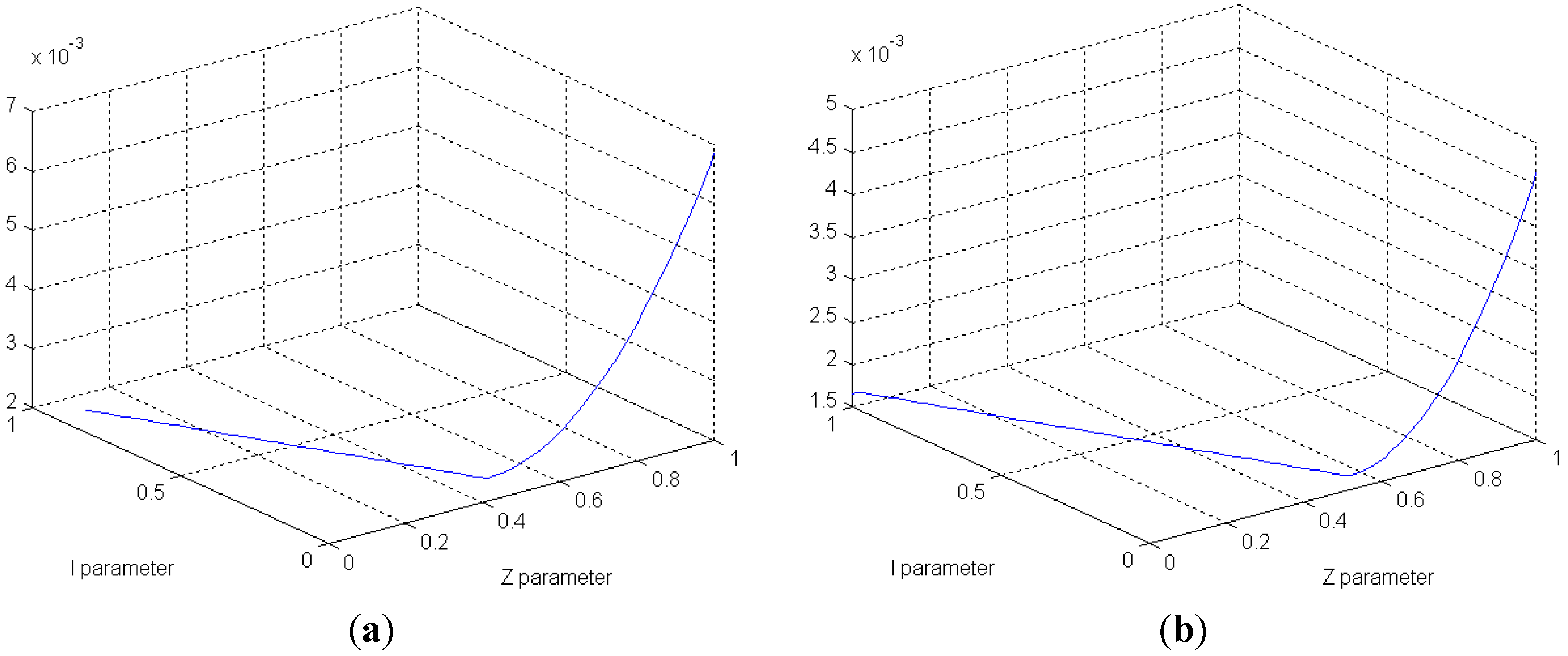
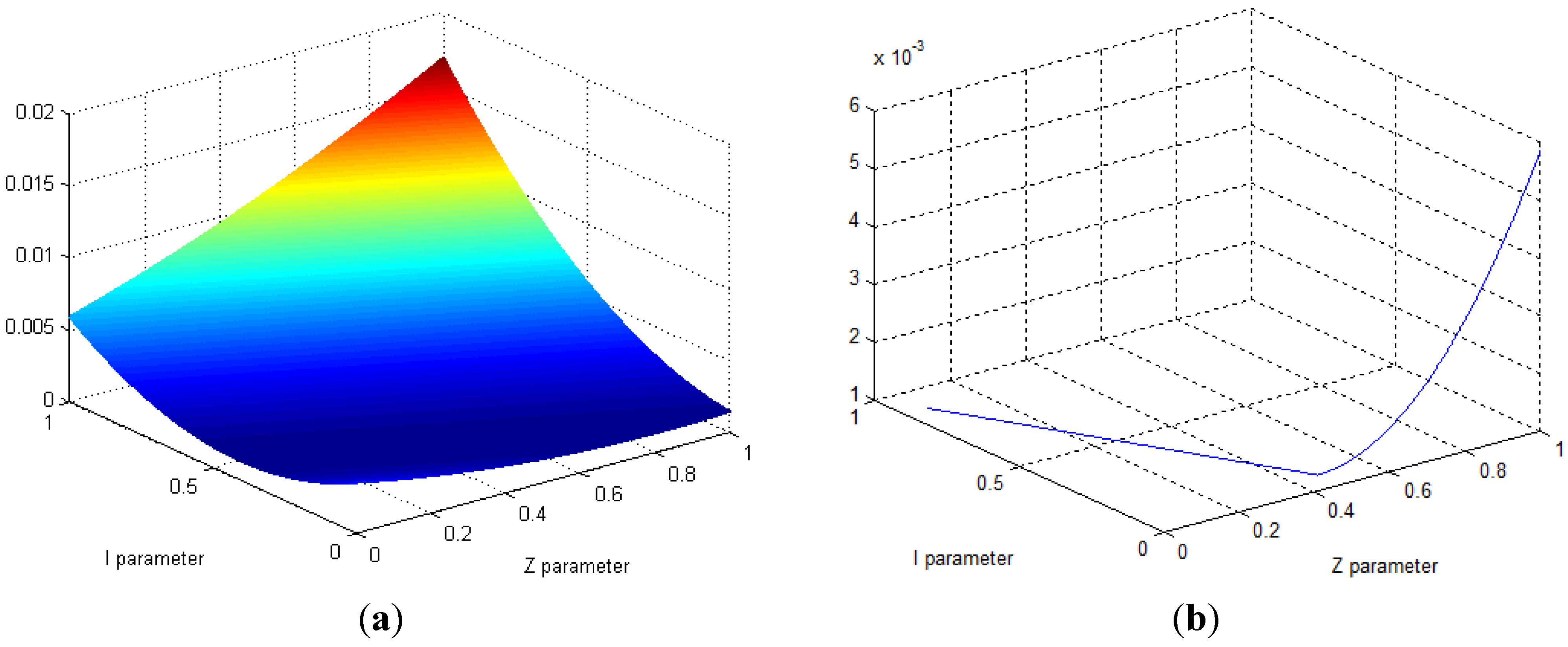
Assuming that the voltage variation is small compared to the nominal voltage, Equation (7) can be simplified to:
Note that Equation (8) is the basic form of linearized load modeling corresponding to the active power consumption of an aggregated load. In Equation (8), pC = 2pZ + pI, and pC is defined as an active linearizing parameter in this paper. Actually, this linearizing parameter can be used as an index to indicate the effect of conservation voltage reduction. When the voltage reduction in Equation (8) is constant, the reduction in normalized active power consumption increases linearly with respect to the active linearizing parameter.
It is reported that conservation voltage reduction is usually executed in the range of 2.0%–5.0% [
25,
26,
27]. Accordingly, in this paper, the upper limit of voltage reduction is assumed to be 5.0%. By comparing Equations (7) and (8), the simplification error is readily seen to be
, and this error is maximized when the load consists entirely of constant impedance,
i.e.,
pZ = 1.0. Therefore, the maximum simplification error is 0.25% for a conservation voltage reduction. Since this error is quite small compared with the normalized active power consumption, it can be neglected, and hence Equation (6) can be simplified to the linearized load model represented by Equation (8). Consequently, the active objective function of Equation (5) can be simplified to:
The equivalence of Equations (5) and (9) means that it is difficult to accurately determine the active ZIP parameters using EMS data resulting from conservation voltage reductions. Instead, only the relationship between the active ZIP parameters (
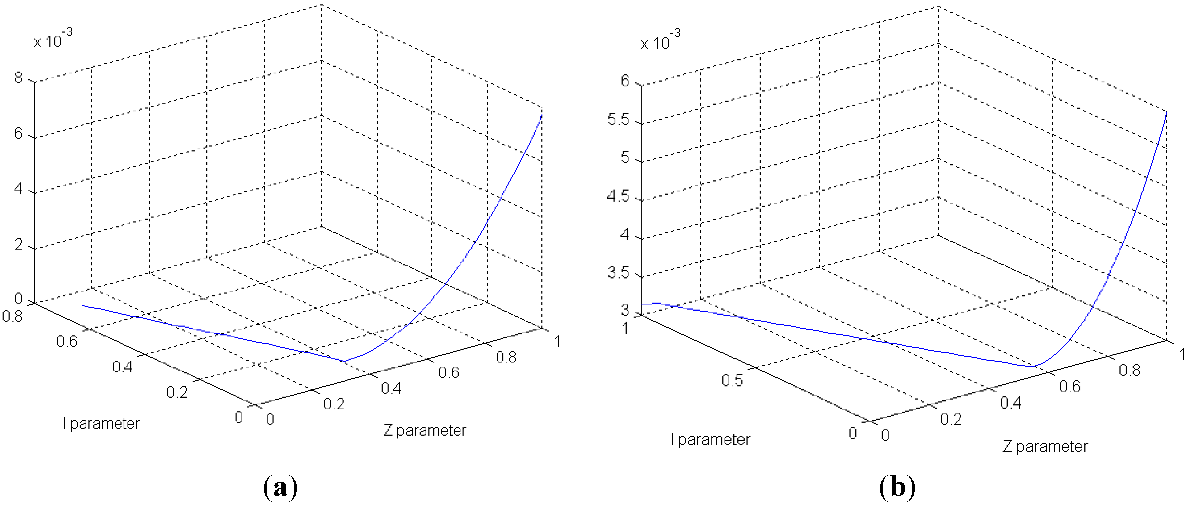
i.e., the active linearizing parameter) can be found. Therefore, when using EMS data resulting from conservation voltage reductions, the active linearizing parameter should be estimated instead of the active ZIP parameters. In a similar manner, the reactive objective function (corresponding to reactive power consumption) can be also simplified to:
where
, and
is defined as a reactive linearizing parameter. Equation (10) is the basic form of linearized load modeling corresponding to the reactive power consumption of an aggregated load. The reactive linearizing parameter should also be estimated using EMS data resulting from conservation voltage reductions.
3. Verification of the Linearized Load Model Using PSS/E Simulations
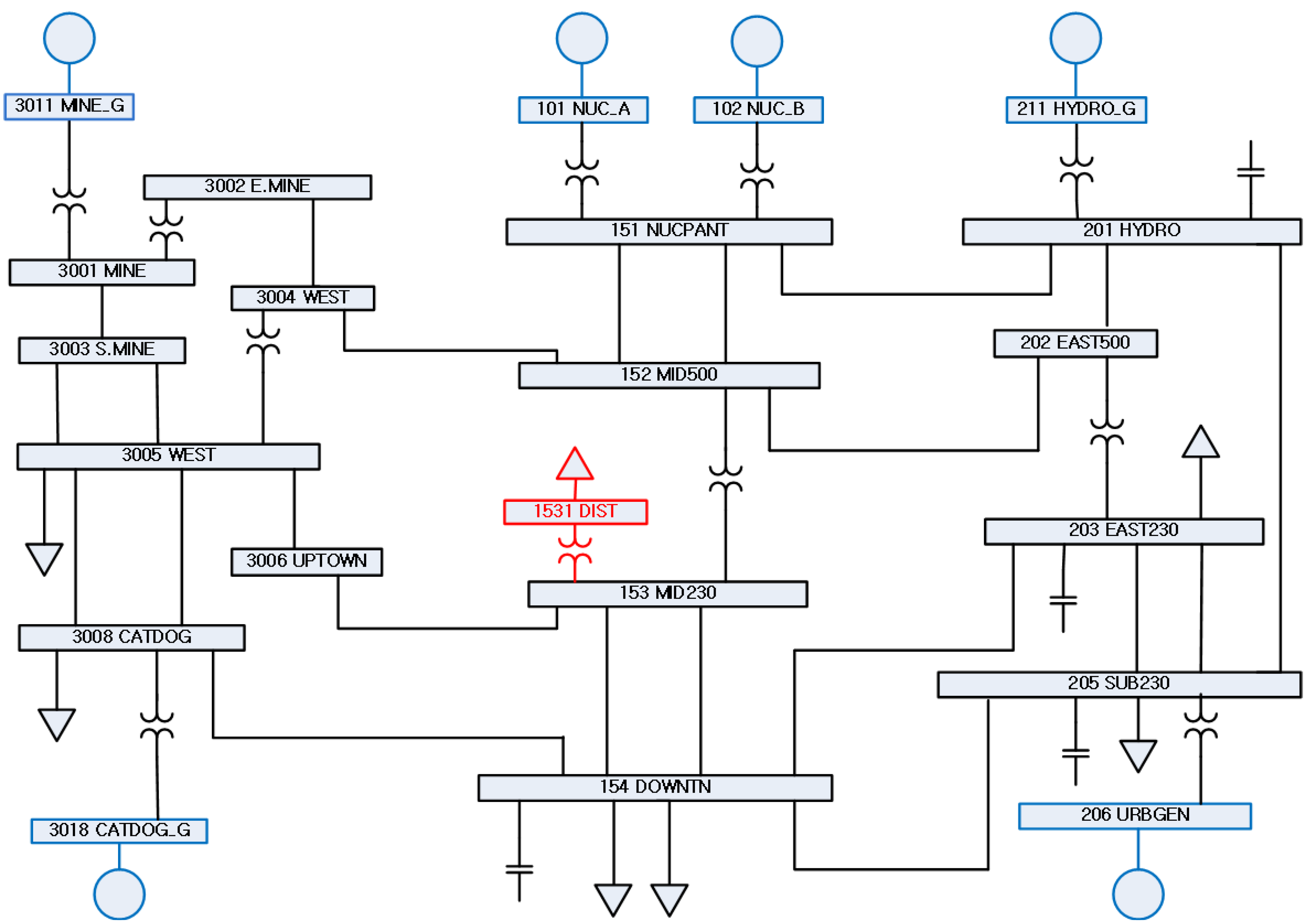
To verify the validity of the linearized load model, PSS/E simulations were performed for a test power system called SAVNW [
28]. The test power system is provided by PSS/E and is depicted in
Figure 1. The base frequency and base capacity were set at 60 Hz and 100 MVA respectively. To evaluate the effect of conservation voltage reduction, the test power system was modified to include a load connected through a distribution transformer. For this purpose, a new distribution bus 1531 was created, and was connected to transmission bus 153 via a distribution transformer with a leakage reactance of 0.1 pu. To preserve the load balance, the original load at transmission bus 153 was moved to the distribution bus 1531.
In the simulations, conservation voltage reductions were executed in two steps. In the first step, a voltage reduction of 2.5% was executed, and an additional voltage reduction of 2.5% was then executed in the second step. At the distribution bus 1531, the initial active power consumption of the load was 200 MW, and its active ZIP parameters were assigned the values , , and , which are typical values used by Korea Electric Power Corporation (KEPCO). To evaluate the effect of the active linearizing parameter on conservation voltage reduction, it was assumed that the active ZIP parameters of the load were unknown, while the active linearizing parameter pC was known to be 0.83. This is because the active linearizing parameter can be estimated using EMS data from conservation voltage reductions, and its value will be 0.83, as pC = 2pZ + pI.
For comparison, two worst cases were considered: the
case (where
pZ has the maximum value) and the
case (where
pI has the maximum value).
Table 1 summarizes the active power variations due to conservation voltage reduction with different active ZIP parameters.
Figure 1.
Test power system.
Figure 1.
Test power system.
Table 1.
Active power variations due to voltage reductions with different active ZIP parameters.
Table 1.
Active power variations due to voltage reductions with different active ZIP parameters.
| Model type | Case | ZIP parameter | Linearizing parameter | Voltage reduction (%) |
|---|
| 0.0 | 2.5 | 5.0 |
|---|
| pZ | pI | pP | pC | Active power (MW) |
|---|
| ZIP Model | KEPCO | 0.350 | 0.130 | 0.520 | 0.830 | 200.0 | 195.9 | 192.0 |
| Linearized Load Model | | 0.000 | 0.830 | 0.170 | 0.830 | 200.0 | 195.9 | 191.8 |
| 0.415 | 0.000 | 0.585 | 0.830 | 200.0 | 195.9 | 192.0 |
In the
case,
pI was set equal to 0.83, as
pC must retain the value 0.83. Consequently,
pZ and
pP were set equal to 0.00 and 0.17, respectively. As
Table 1 indicates, the active power savings in this case were almost identical to those of the actual ZIP model. With a 5.0% voltage reduction, the active power error was only −0.104%. In the
case, the active ZIP parameters were assigned the values
pZ = 0.415,
pI = 0.000 and
pI = 0.585. As in the
case, the active power savings were almost identical to those of the actual ZIP model.
At the distribution bus 1531, the initial reactive power consumption of the load was 100 MVAR, and its reactive ZIP parameters were assigned the values
qZ = 0.56,
qI = 0.08 and
qP = 0.36, which are also typical values used by KEPCO. As in the active power cases, it was assumed that the reactive ZIP parameters were unknown, but the reactive linearizing parameter
qC was known to be 1.20. This is because the reactive linearizing parameter can be estimated using EMS data from conservation voltage reductions, and its value will be 1.20 because
qC = 2
qZ +
qI.
Table 2 summarizes the reactive power variations due to conservation voltage reductions with different reactive ZIP parameters. In the
case,
was set equal to 0.80, as (2
qZ +
qI) must retain the value 1.20, and (
qZ +
qI) should not exceed 1.00. Consequently,
and
were set equal to 0.20 and 0.00, respectively. As
Table 2 indicates, the reactive power savings in the
case were almost identical to those of the actual ZIP model. With a 5.0% voltage reduction, the reactive power error was only −0.106%. In the
case, the reactive ZIP parameters were assigned the values
,
, and
. As in the
case, the reactive power savings in the
case are almost identical to those of the actual ZIP model.
Thus, it was demonstrated that the linearized load model is sufficient to accurately evaluate the effect of conservation voltage reduction.
Table 2.
Reactive power variations due to voltage reductions with different reactive ZIP parameters.
Table 2.
Reactive power variations due to voltage reductions with different reactive ZIP parameters.
| Model type | Case | ZIP parameter | Linearizing parameter | Voltage reduction (%) |
|---|
| 0.0 | 2.5 | 5.0 |
|---|
| qZ | qI | qP | qC | Reactive power (MVAR) |
|---|
| ZIP Model | KEPCO | 0.560 | 0.080 | 0.360 | 1.200 | 100.0 | 97.10 | 94.20 |
| Linearized Load Model | | 0.200 | 0.800 | 0.000 | 1.200 | 100.0 | 97.00 | 94.10 |
| 0.600 | 0.000 | 0.400 | 1.200 | 100.0 | 97.10 | 94.20 |
4. Modeling Aggregated Loads Based on EMS Data
Korean EMS data were used to estimate the linearizing parameters for the loads in an actual power system. These data are sampled every 4 s from 1746 transformer banks at the various substations. Since raw Korean EMS data are saved for each individual transformer bank, aggregated loads were modeled for each of them. To find the linearizing parameters for the aggregated loads, more than two sets of conservation voltage reduction data are required for each transformer bank, and thus it was assumed that the transformer bank loads have the same linearizing parameters for the same season and time of day. The raw EMS data were divided into four groups according to the season: spring (March–May), summer (June–August), fall (September–November), and winter (December–February). Each group was subdivided into three subgroups according to the time of day: daytime (08:00–16:00), evening (16:00–24:00), and night (24:00–08:00).
Details of the data acquisition process are described in [
14]. The voltage, active power, and reactive power are continuously monitored by a data acquisition program connected to the Korean EMS. The data are saved when the voltage variation is greater than 1% (six samples before voltage variation, and 20 samples afterwards). The saved data are periodically checked and are utilized to find the linearizing parameters for the transformer bank loads.
5. Conclusions
This paper proposed an EMS-data-based static load model for evaluating the effect of conservation voltage reduction at a national level. Because EMS data are saved for each transformer bank, an aggregated load model is required to use these data for static load modeling. Although a ZIP model is one of the most appropriate load models due to its simple structure and practicality, it cannot be used for aggregated load modeling based on EMS data resulting from conservation voltage reductions. Given that conservation voltage reductions are usually executed in the range of 2.0%–5.0%, it is difficult to accurately determine ZIP parameters using EMS data obtained from conservation voltage reductions. Therefore, this paper introduced a linearized model for aggregated static loads. In this linearized model, the active and reactive linearizing parameters are estimated for the active and reactive loads, respectively, using EMS data from conservation voltage reductions. Since EMS is widely used in modern power systems, and its data are readily available, the linearized load model can be used to evaluate the effect of conservation voltage reduction without installing additional measuring devices.
To verify the validity of the linearized load model, PSS/E simulations were conducted for a test power system, and the linearized load model was found to be sufficient to accurately evaluate the effect of conservation voltage reduction. Korean EMS data were used to estimate the linearizing parameters for transformer bank loads in an actual power system. Assuming that the transformer bank loads have the same linearizing parameters for the same season and time of day, raw EMS data were divided into four groups according to the season, and each group was subdivided into three subgroups according to the time of day. The linearizing parameters were estimated using EMS data for each subgroup. As expected, the estimation results for the linearizing parameters varied according to transformer bank, season, and time of day. Thus, to evaluate the effect of conservation voltage reduction, linearizing parameters must first be accurately estimated for each transformer bank, season, and time of day. For this purpose, EMS data are continuously being accumulated. Once a sufficient quantity of EMS data has been secured, it will be possible to evaluate and forecast the effect of conservation voltage reduction via linearized load modeling.

 ,
, 


