1. Introduction
Development in Brazil has been paired with an increase in energy and electricity use both
per-capita and overall demand [
1]. While Brazil currently generates 65% of its electricity from hydropower, increasing demand and the diminishing quality of dam sites will likely increase the generation from other sources. All electricity generation options, including additional hydropower, contribute to environmental impacts such as climate change, land transformation, and water quantity/quality. In examining shifts to new generation sources, impacts from construction and fuel production need to be considered at the same time as impacts from generation. While existing models and studies have assessed effects of low-carbon scenarios, they often omit impacts (e.g., emissions from hydroelectric reservoirs) or consider a limited set of impacts or life-cycle stages (e.g., ignoring construction). With the expectation of significant additional generating capacity and the need to consider limited resources such as water and land, a broader approach is required for effective energy or environmental policy.
The goal of this work was to calculate and examine environmental impacts from electricity generation in Brazil as generation sources shift over the coming decades. While previous work has generated life-cycle assessment (LCA) data for electricity sources, and described paths forward for Brazilian electricity, tools to combine these datasets in a region-specific and/or annual manner have not yet been created. In examining impacts, there is particular interest in assessing whether likely scenarios will enable Brazil to meet carbon reduction targets, and how changes in the use of hydropower may affect land and water resources, with the goal of suggesting areas where policies can effect change. This work discusses these questions through developing a robust model for calculating annual environmental impacts under a given generation scenario. This model is generalizable to other regions, energy and water services, and questions than this specific application.
1.1. The Brazilian Electricity Grid
Brazil has 84 GW of installed hydroelectric capacity as of 2012, and 130 GW total installed electrical generating capacity [
2,
3]. However, most high-quality dam sites, particularly in the more populous southern half of the country, have now been developed [
4]. Thermal power plants, mainly from natural gas, coal, nuclear fission, and biomass, represent 28% of the Brazilian power grid—with a large amount of biomass electricity used internally rather than exported onto the main power grid. The remaining 6% of generation imported, primarily from Paraguay. Brazil currently has limited installed solar or wind generation capacity, but is planning to construct 3 GW of wind capacity in the coming years [
2].
Brazil’s population increased by a factor of two between 1971 and 2008, but
per-capita electricity use increased by a factor of five [
5]. 96.6% of the country is connected through the National Interconnection System (SIN), with
per-capita electricity consumption driven by increasing income and available technology. Brazil’s electricity has a lower carbon intensity than that of many countries, with 208 kg CO
2/MWh
vs. the U.S. average of 748 kg CO
2/MWh [
6], but the system will require expansion to meet future demands. Increases in generating capacity are expected to come from four major sources: hydropower in the Amazon River basin, natural gas, biomass, and renewables. New Amazonian dams may flood large forest areas, have less steady water supplies, and have increased emissions from decomposition [
7]. Dam sites are also likely to be further from major population centers, increasing transmission losses. While current dams have ongoing environmental impacts, much of their impacts, such as concrete and steel manufacturing, are embedded from construction, providing time-dependent advantages in cost and energy consumption when compared to new supplies. Greenhouse gas (GHG) emissions, as shown in the LCA data used in this paper, are highly uncertain and variable [
8]. Natural gas (NG), one of the primary large-scale alternatives to hydropower, currently has limited domestic supplies. New supply prospects include associated production from the pre-salt offshore oilfields or shale gas basins, increased pipeline capacity, or increased liquified natural gas (LNG) imports. NG is also an insufficient response to the problem of climate change [
9]. Expanded use of biomass in the form of sugarcane bagasse for electricity production uses a renewable fuel, but requires significant land and is available at a finite annual rate. Questions of which sources to pursue or encourage require new tools to integrate multiple sets of data, particularly when considering future environmental impacts.
1.2. Scenario Analysis
Scenario analysis is distinct from forecasting methods in that scenarios are based on stated assumptions about social, economic, and environmental conditions in the future, rather than extrapolation from present trends. Scenario analysis allows for the examination of specific policies or hypotheses, not only to assess lower costs or impacts, but also to identify key impact drivers or time points. Past scenario-based work focusing on Brazil has examined the impacts of climate change scenarios on effective use of renewable energy sources [
10], the potential for carbon abatement in industry [
11], and scenarios for implementation of solar photovoltaics [
12]. The cost optimization model used in this work, the Model for Energy Supply System Alternatives and their General Environmental Impact (MESSAGE), is managed by the International Atomic Energy Agency (IAEA) and has been used to examine scenarios in many countries [
13,
14,
15,
16,
17,
18], including studies focusing only on low-carbon scenarios for Brazil [
19,
20]. Existing studies, while including land use, did not consider impacts beyond greenhouse gases, and did not incorporate hydroelectric reservoir emissions due to high uncertainty. A broader set of impacts and time-dependence for major impact drivers is necessary for fully informed policymaking and energy planning.
1.3. Life-Cycle Assessment
Life-cycle assessment (LCA) is an established method for quantifying impacts over the entire life cycle of a product, process, or service, including both direct impacts from the use phase (e.g., electricity generation) and indirect impacts from upstream supplies and processes or waste management. LCA has been codified by several organizations including the International Organization for Standardization’s (ISO) 14040 set of standards [
21], and includes four steps: goal and scope definition, inventory collection, impact assessment, and interpretation. Conventions for these steps vary by topic, with significant portions of inventory collection and impact assessment often performed using pre-existing and established databases and tools [
6,
22,
23,
24]. Uncertainty throughout the process is often handled via Monte-Carlo (MC) methods, which sample distributions for key parameters for many trials to generate a final distribution [
25,
26].
2. Methods
The model presented here used LCA data, current regional electrical generation infrastructure and geographic conditions, and information from constructed MESSAGE scenarios to calculate the total environmental impacts of supplying electricity to Brazil from 2010 to 2040 [
27]. The functional unit was the MWh of electricity required for each year, with the system boundaries including all processes up to electricity distribution to the nationwide grid. This boundary was equivalent to calculating producer impacts and costs before taxes and distribution. Efficiency of local distribution and use were not considered, and no systematic regionalization of results was performed.
Data collection, with an emphasis on LCA data, and basic modeling assumptions are discussed in
Section 2.1. The scenarios used in this study were projected with the MESSAGE model based on an existing version developed by [
28]. The base case identified a cost-optimal path to meet predicted demand through 2040, while the four side cases examined the sensitivity of the base case to decreased electricity from biomass or increased solar power production. Background on the MESSAGE model and the various cases considered are discussed in
Section 2.2. The calculation procedure for the model itself is described in
Section 2.3, with an overview of the data structures provided below. The wide variety of data sources introduce uncertainty and variability, calculated via Monte-Carlo (MC) methods. The MC methods and validation of model results for GHGs are discussed in
Section 2.4.
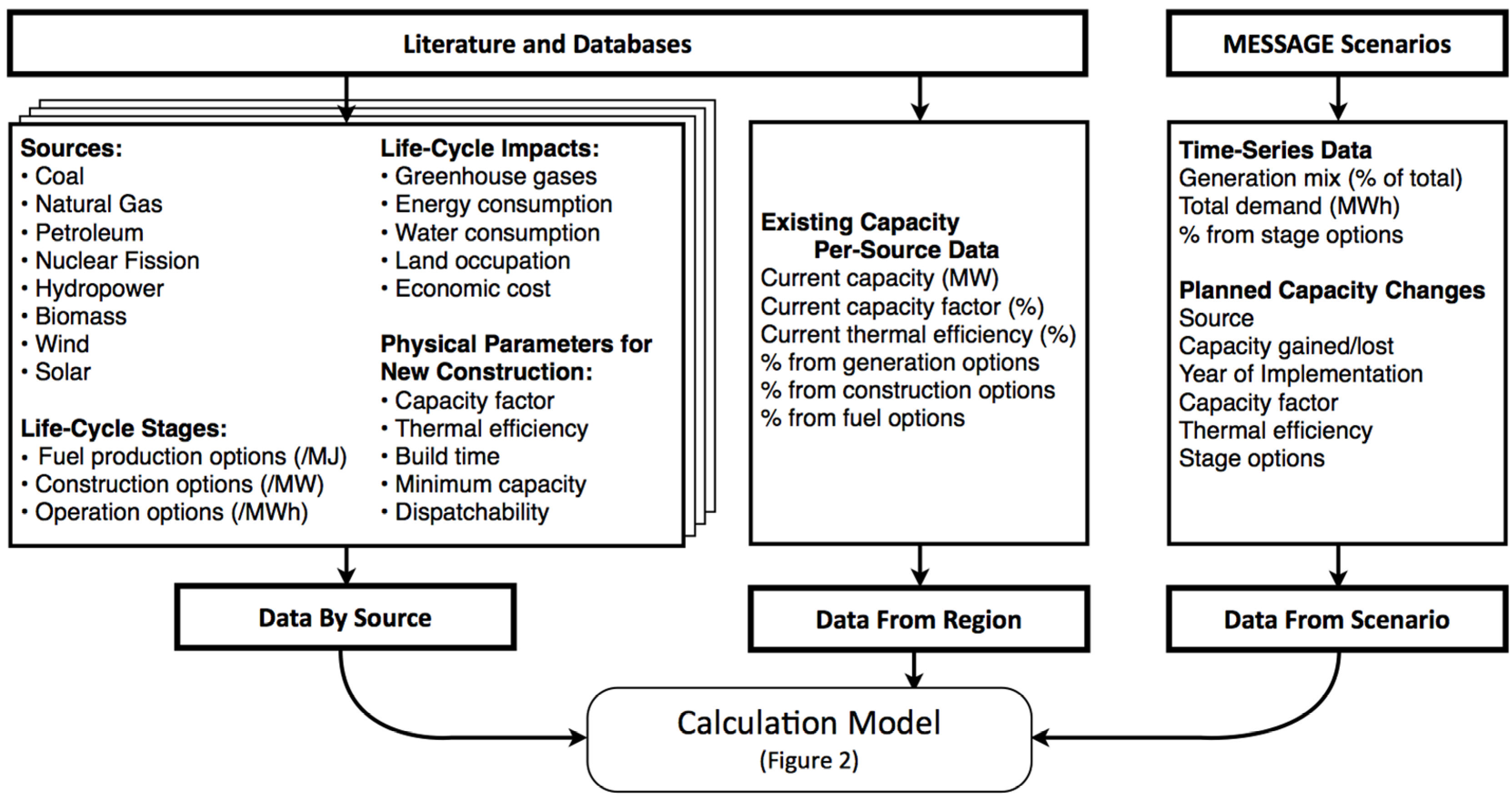
The input data for the LCA model are shown in
Figure 1, with the three categories of data—source, region, and scenario—acting as the starting point for the calculation procedure, which is shown in
Figure 2. The LCA model divided information along four areas: time, eight sources, three life-cycle stages, and five life-cycle impacts. The eight basic electricity sources included were coal, natural gas, petroleum, nuclear fission, hydropower, biomass, wind, and solar (with both photovoltaics and thermal power plants). For each source, we collected data on three life-cycle stages: fuel production, construction of new generation capacity, and operations. Fuel production included impacts for growing or extracting, processing, and delivering fuel for combustion. Construction included production of necessary materials, installation, and total capital costs. Operations included combustion emissions for thermoelectric sources, operations and maintenance requirements, and financing costs. Many sources have multiple options for one or more stages, either different methods—e.g., surface
vs. underground mining, or open
vs. closed loop cooling—or different regions where geographically dependent sources such as hydropower or wind energy will perform differently. We collected information on each option’s unique environmental impacts. The annual percentage of a source or stage from each option was defined by the scenario.
Impacts were calculated in five categories: Greenhouse gases (GHGs), combined using 100-year global warming potential [
29], energy consumption, water consumption, land occupation, and economic cost. Energy consumption considered total primary energy required, not including the energy value of the fuel itself. Water consumption was calculated based on volume of water not returned to a withdrawal source, irrespective of quality. Land occupation was the physical area of land used for a given process, without consideration of changes in quality. Economic cost was calculated in 2010 U.S. Dollars, using the 2010 average conversion rate from Brazilian Reais of 1.838:1 where necessary [
30].
Figure 1.
Model data sources and input requirements. The data sources and inputs were used in the calculation model in
Figure 2.
Figure 1.
Model data sources and input requirements. The data sources and inputs were used in the calculation model in
Figure 2.
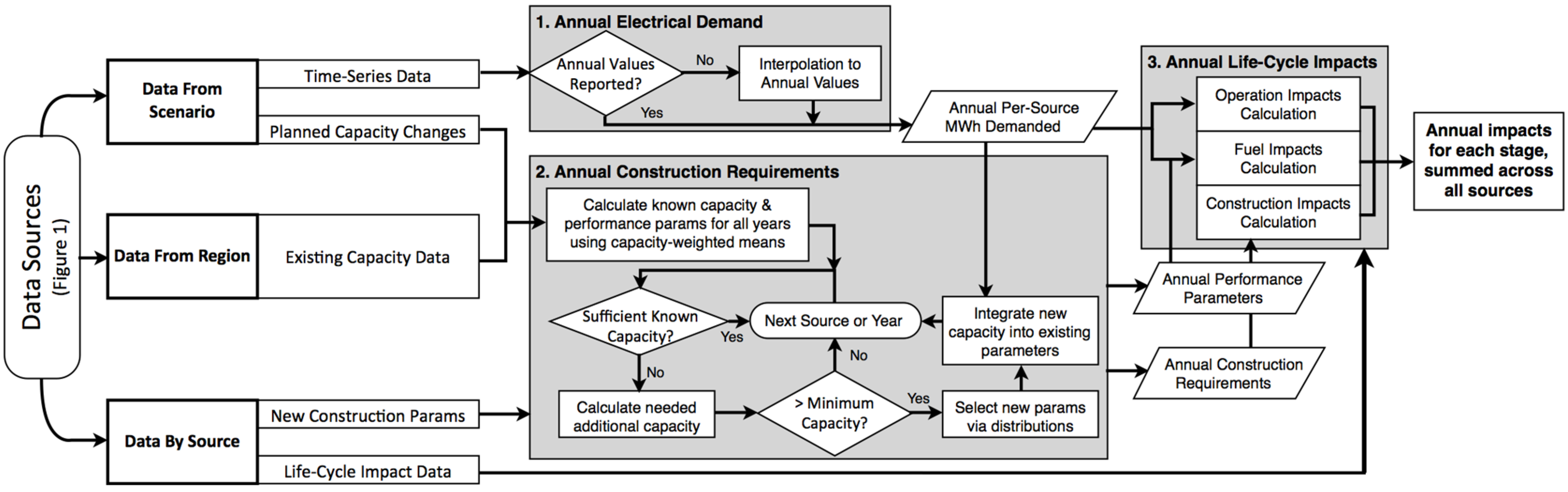
Figure 2.
Calculation model, using data inputs from
Figure 1. Grey areas indicate calculation sections (With calculation Section X described in
Section 2.3.X).
Figure 2.
Calculation model, using data inputs from
Figure 1. Grey areas indicate calculation sections (With calculation Section X described in
Section 2.3.X).
2.1. Life-Cycle Data and Source-Specific Modeling Assumptions
LCA data was collected from existing databases such as ecoinvent 2.1 and U.S. LCI [
6,
22]; government agencies including the Brazilian Ministry of Mines and Energy (MME) and National Electricity Agency (in Portuguese, ANEEL) [
31,
32]; and existing literature [
33,
34,
35,
36]. Databases were used when processes technologically appropriate and contained sufficient information for disaggregating stages. For many newer sources such as biomass, wind, and solar power, literature sources provide more updated information. Data on power plant construction costs were taken from studies by the Electric Power Research Institute (EPRI), National Renewable Energy Laboratory (NREL), and the Energy Information Administration (EIA), and were accessed using the OpenEI tool [
37,
38,
39]. The full listing of LCA data sources can be seen in
Table A1, with a table of median unit impacts and distributions available in
Table A2.
Many data were only available for the United States or Europe and it was assumed that Brazilian plants are—and will continue to be—similar in materials and methods of operation to those in Europe and the U.S., with performance parameters taken from current Brazilian conditions. The power sources with the most variation relative to U.S. or European impacts were hydropower and biomass combustion, as noted by Coelho [
40]. Our general approach to modeling hydropower-related emissions is detailed below, with specific assumptions for all other sources found in
Table A3.
Hydropower
Land Use. Brazilian hydroelectric dams were generally constructed primarily for electricity generation; allocation for co-products such as irrigation, navigation, and flood control is less appropriate than in other countries [
41]. We assigned all impacts from reservoir emissions and dam construction to electricity, consistent with previous studies [
42]. To account for the wide variation in land use, we separated dams into temperate and tropical categories. After collecting information on reservoir size for 31 dams based on Eletrobras and ANEEL information, we calculated distributions in km
2/MW for both regions [
2,
43]. For each new dam, an impact factor was selected from the appropriate distribution based on the dam’s probable location (increasingly weighted towards tropical regions over time), and included in the regional unit impact factor for each year based on capacity-weighted means. This approach separates the natural variability in reservoir size from simple uncertainty in LCA impact factors. Water consumption due to reservoir evaporation was based on Brazilian results from Pfister
et al., with an assumption of 10% uncertainty [
42].
In addition to direct land use by reservoirs, energy projects can also induce further land use changes. For hydropower, this induced change is likely to come from additional development around the dam and reservoir, in addition to replacement of previous cleared and now flooded areas. Hydropower-induced land use changes have not yet seen significant work, and are likely to be site-specific. The magnitude of the reservoirs relative to other uses in the lone available study suggests that extra land cleared for development around hydropower dams will represent a small fraction of the total impact [
44]. For irrigation-focused dams, this ratio may vary. Because of the uncertainty in this area, we did not include induced land use change, but did perform a sensitivity analysis based on the fraction of reservoir land area that was developed as a result of inundation.
Reservoir Emissions. The impacts of hydroelectric dam operations and maintenance were included via data from ecoinvent [
6]. While the powerplant itself does not generate GHG emissions, there are several pathways related to the reservoir and power generation that may release either CO
2 or CH
4. Three major pathways have been described by other researchers [
7,
36,
45,
46]: CH
4 and CO
2 bubbling from decomposed biomass, gases diffusing to the surface, and gas released via the pressure drop when water is pulled through the dam’s turbines (degassing). The studies that have examined CO
2 and CH
4 emissions from Brazilian reservoirs have identified high emissions in several tropical cases, and agree that these emissions are significant and currently excluded from most studies [
33,
36,
45,
46,
47,
48].
However, measurements to date have only managed to assess gross emissions, and information about net emissions for the reservoir area before and after flooding are highly uncertain. Some biomass that decomposes in reservoirs flows from upstream sources, and would have decomposed regardless of the dams’ existence, though more methane may be produced because of a longer and deeper retention. In tropical regions, the lower land gradient and seasonal rainfall can expose and flood large amounts of land, producing annual decomposition within the reservoir area in addition to decomposition of initially flooded material [
49], providing long-term net emission increases. Other changes in net emissions concern land use—while rivers can be net sources of GHGs, surrounding forest land are generally considered to be net carbon sinks [
46], and the reduction in carbon uptake is effectively a net emission.
Impact factors for reservoir GHGs were calculated in the same manner as with land use for infrastructure, with starting values of 29 kg CO
2-eq/MWh and 543 kg CO
2-eq/MWh for temperate and tropical dams, respectively, and distributions for GHGs of future dams based on existing research cited above [
36]. This provides an estimate of gross reservoir emissions. Assuming that net emissions are some fraction of gross emissions but still positive, we calculated and reported reservoir emissions separately from other GHGs impacts for three cases: a low case where net emissions were 10% of gross emissions, a median case where they represented 50%, and a high case where they represent 90% of gross emissions. These bounds give some estimate of a very high uncertainty, which will require additional field-work for characterization.
2.2. MESSAGE Scenarios
The electricity scenarios used in this work were based on the coupling of the IAEA’s demand component (MAED) and MESSAGE models. The two models combine top-down assumptions, such as economic and population growth, bottom-up disaggregated sectoral information, and constraints related to energy resource availability to produce energy demand and optimal energy supply scenarios. The demand component (MAED) provides detailed sectoral energy demand projections while a linear programming energy supply optimization model (MESSAGE) provides the least-cost energy and electricity supply mix scenario. For further information, see [
18]. The MAED-MESSAGE models have been applied in several different energy studies [
17,
18,
20,
27,
50,
51]. The models were used in this study to create future scenarios for the electricity sector in Brazil. The premises for this work, as well as the central structure of the Brazilian implementation of MESSAGE, were derived from Borba [
28].
Five scenarios were developed using MESSAGE: one reference case and four side cases, based on more or less intensive implementations of biomass and solar technology. The reference case has been used in previous work in a different context; the side cases were developed for this study. The reference case was an attempt to simulate a business as usual (BAU) trajectory for the Brazilian energy system, and shows demand rising from 500 TWh in 2010 to 1100 TWh in 2040, with natural gas and biomass generation expanding to meet much of this demand. Increases in these two sources are cost effective and widely expected [
3,
52,
53].
The side cases were developed to represent sensitivity analyses aimed at assessing two specific energy technologies: hydrolysis for ethanol production and solar power. All side cases maintained the same demand growth to 1100 TWh in 2040, shifting only the generation mix to meet demand. Two scenarios were developed for each technology, to examine a basic
vs. intensive approach. The basic side cases were solved using the MESSAGE model, with the more intensive versions produced by magnifying the shift in per-source generation between the base case and the side case by a constant factor. In the first side case (BIO), an increase in second generation ethanol production from hydrolysis of sugarcane bagasse was forced into the model to assess the implications for decreased availability of biomass for electricity generation.
Table A4 depicts the premises about increase in ethanol production from hydrolysis in the BIO scenario. The hydrolysis case was magnified by 1.5 to produce the BIO2 scenario, with use of a higher factor limited by a desire to have zero or positive electricity production from biomass.
The second side case (SOL) evaluated increased participation of solar energy in the electricity generation mix. Wind power, another commonly discussed alternative, is a cost-effective option and expands without assistance in the cost-optimal BAU case. In contrast, solar technologies are not yet low-cost enough to be selected by the MESSAGE model. To examine their potential, a combination of solar electricity generation technologies were forced into the model, with cost optimization for meeting the remaining demand. In 2040, solar technologies were responsible for generating an arbitrarily chosen 4.0% of total demand. The technological alternatives were: concentrating solar power, CSP with 12 or 6 h heat storage (CSP 12 h and CSP 6 h), photovoltaic (Solar PV), solar and bagasse hybrid CSP plants (Solar Hib).
Table A5 shows the penetration of solar energy technologies in the SOL scenario. The SOL case was magnified by 2 to produce the SOL2 scenario, which generates 8.8% of electricity from solar technologies in 2040. Both of the SOL cases represent a policy-driven change without a specifically noted physical boundary.
All three basic scenarios were generated using optimization for economic cost, with the basic side cases optimizing cost for all unforced generation requirements. The more aggressive side cases magnified the effects of the basic ones on per-source generation requirements. The initial and final requirements for all five cases are shown in
Table 1. Both side cases were conducted in order to test alternative pathways for the Brazilian energy sector as the result of directed energy policies. The side cases differ from the reference case in that they were not least cost pathways, since they do not encompass the optimal solution for the evolution of the electricity sector. On the contrary, they were alterations from the least cost scenario built specifically to illustrate the potential and applicability of the LCA methods by providing examples of how this model can be used to evaluate the results of energy policies directed at incentivizing specific technologies.
Table 1.
Demand requirements during 2010 and 2040 for each case. The business as usual (BAU) case was cost-optimal, while the BIO and SOL side cases were cost-optimized outside of forced changes to biomass and solar usage. The BIO2 and SOL2 cases were magnifications of the difference between the BAU case and respective side cases to examine response linearity in the calculation model. Bolded values show major changes between the BAU and side cases.
| Source | All | BAU | BIO | BIO2 | SOL | SOL2 |
|---|
| Year | 2010 | 2040 |
|---|
| Total demand (TWh) | 500 | 1100 | 1100 | 1100 | 1100 | 1100 |
| Coal | 2.4% | 2.9% | 2.8% | 2.8% | 2.9% | 2.9% |
| Natural gas | 15% | 23% | 28% | 31% | 20% | 17% |
| Oil | 0.4% | 0.0% | 0.0% | 0.0% | 0.0% | 0.0% |
| Nuclear | 3.0% | 2.0% | 2.0% | 2.0% | 2.0% | 2.0% |
| Hydro | 76% | 61% | 61% | 61% | 61% | 60% |
| Biomass | 3.2% | 8.1% | 2.9% | 0.3% | 8.1% | 8.1% |
| Wind | 0.3% | 3.2% | 3.2% | 3.1% | 3.1% | 3.1% |
| Solar | 0.0% | 0.0% | 0.0% | 0.0% | 3.7% | 7.5% |
| Total | 100% | 100% | 100% | 100% | 100% | 100% |
2.3. Calculation Procedure
The calculation process for the model is shown in
Figure 2 and consisted of three aggregated steps, outlined in grey: (1) calculation of per-source annual electrical demand; (2) identifying necessary annual construction requirements to meet deman; and (3) combining these two requirements with LCA data to calculate annual life-cycle impacts in the five impact categories. An example of input data, based on the scenarios used in this work, and the fixed parameters for each source can be found in
Table A6 and
Table A7. Specific input data for the calculations are shown in
Figure 1 by scenario, region, and source.
2.3.1. Annual Electricity Demand Requirements
Electricity demand requirements were calculated in two sections: generation mix and total quantity in MWh. The generation mix was defined as the fraction of electrical demand from each source in a given year. The total quantity was defined as the MWh required over the entire country for a given year. The MESSAGE model provided values for both sections for every 5th year, with intermediate values for generation mix and total quantity calculated using linear interpolation. With the annual generation mix and demand, total per-source demand was calculated in MWh.
Two adjustments were made to generation requirements. For solar and wind power, generation was based on installed capacity and capacity factor, with scenario requirements as a minimum amount. Excess generation was offset by reductions in natural gas generation requirements, and at the low penetrations seen in the scenarios, curtailment from excess power production was not expected to be significant. For hydroelectric power, natural variability in river flow was included by adjusting hydropower generation requirements by a random percentage selected from a normal distribution with standard deviation varying between 5.4% and 12%, depending on the ratio of temperate and tropical capacity. These values are based on annual per-generator MWh from the Itaipu and Tucuruí dams since 1995. Excess or insufficient generation was assumed to be offset by natural gas.
No adjustments were made to generation requirements to account for daily or seasonal variation in electrical demand or renewable energy sources. The widespread use of hydropower and natural gas offer the capacity to balance these variations, even at higher penetration rates for wind and solar power. Time-balancing is below the temporal resolution of this work, but is an important topic for future work (see
Section 4).
2.3.3. LCA Impacts Calculation
LCA data were collected for each source, stage and option, forming 160 independent points (8 sources × 3 stages × 5 impact categories + options). Distributions were developed for each point, with unit values (impacts per MWh of generation, MW of capacity, or MJ of fuel) selected once for each point and held constant for all years. See
Section 2.4 for details on the development and use of the distributions.
Using Equation (2), unit impacts for each option
j were combined into a single unit value for each source
s, year
t and stage
g, with
I as the vector of unit impacts and
f as the fraction from each option of a source and stage, and in a given year. Fractions were defined starting from current practice, with new construction adjusting them proportional to capacity.
To calculate final environmental impacts, each year’s 24 output vectors from Equation (2) (eight sources with three stages each) were combined with annual generation and construction requirements for each source. Operational impacts were calculated from required per-source demand. Construction impacts were calculated based on constructed capacity for each source. Fuel production impacts were calculated based on per-source demand, and adjusted for annual thermal efficiency relative to a reference value used for collecting LCA data. Land occupation from existing infrastructure was calculated during the first year of the scenario, with future construction impacts added to this initial value as land is occupied but not consumed. Combining the cumulative land occupation from infrastructure with occupation from operational impacts produced total annual land occupation.
2.4. Uncertainty and Validation
To incorporate uncertainty and variability, Monte-Carlo methods were applied to two sets of data during calculations: performance parameters and unit life-cycle impacts for each stage and source. Capacity factors, thermal efficiencies, and stage options were selected from distributions or probabilities when new power plants were added. The distributions were developed from current practices and future technology characterizations; sources are shown in
Table A1. Although capacity factor is normally a function of demand, dispatch order, and operational cost, this model assumed that new construction will contribute capacity operating at a selected capacity factor as part of a wider set of power plants.
While performance parameters vary year to year for the same source within a trial, unit LCA values for all sources, stages, and options were chosen once for all years of a given trial. The distributions for all values were either normal, lognormal, triangular, or uniform, depending on data availability—for values from ecoinvent and some literature sources, more robust distribution data were available and normal or lognormal values were used. In the case of ranges, uniform distributions were used, and for sources that reported a range with a central value, triangular distributions were used as a conservative approach. Many estimates remain as point estimates due to a lack of harmonized data in several impact categories, particularly energy consumption. The use of MCA with LCA data was largely to assess uncertainty in LCA data rather than variability between power plants, resulting in the use of the same LCA impact values for the entire trial.
The two-part Monte-Carlo approach targeted two separate sources of variability: uncertainty in the life-cycle impact data that would affect all years in a similar manner, and variability in the implementation of technology that changed impacts every time a new power plant was built. For hydroelectricity, both uncertainty in LCA impacts and variability for new plants were included by adjusting the unit LCA impacts for each new hydroelectric dam.
Annual impacts for each of the five categories were combined from a per-source basis into both overall impacts and per-stage impacts for operations, construction, and fuel production impacts for each trial. After 4000 trials were calculated, the 5th, 50th, and 95th percentiles for each year and stage were reported. This approach reports the median rather than the mean, eliminating the effect of high-impact trials skewing results upwards, with the side effect of minimizing worst-case scenarios. The use of 4000 trials was found to have variation between model runs of <0.1% for all categories.
Results were validated by comparing 2010 model results for GHGs to World Bank data on GHG emissions from energy [
5] and to GHG emissions calculated from the Brazilian Government’s National Energy Balance (BEN) [
54]. Values for both methods and model results are visible in
Table 2; World Development Indicator data is available through 2008 and was extrapolated to 2010. The 2010 total value is from a World Bank report on low-carbon Brazilian land use and energy scenarios, and matches the sum of the three independent categories [
19]. For a second reference/validation point, energy-related GHGs were calculated using emission factors and 2010 energy usage from the BEN. Electricity’s GHGs were calculated using EIA combustion factors, which exclude any impacts from reservoirs. Finally, model results for electricity were reported with the average of the heating and transportation values from the two methods so that total energy-related GHGs could be compared.
Table 2.
Comparison of business as usual (BAU) results to existing data for validation. Italics are used to show calculated or extrapolated values, while non-italic values are directly from sources. All values are in million metric tons (Mt) of CO2-eq. The model factors for this work do not include impacts from hydropower reservoirs.
| Source | Year | Electricity | Heating | Transport | Total |
|---|
| World Bank [5] | 2005 | 59 | 34 | 136 | 229 |
| World Bank LU, [5,19] | 2010 | 64 | 39 | 152 | 256 |
| BEN calculations [54] | 2010 | 58 | 40 | 168 | 266 (EIA) |
| 2010 BAU model results (this work) | 2010 | 50%: 66; 5%: 45; 95%: 86 | 39 | 160 | 286 |
The model results include indirect non-combustion emissions, increasing electricity GHGs from our results in comparison to the two validation datasets. While reservoir emissions were included in the model, they were not compared during this validation phase, and were separated out for results reporting due to high uncertainty. The inclusion of separate values for the GHGs of tropical and temperate reservoirs produces a per-MWh value for hydropower of 50 kg CO2-eq/MWh and gross emissions from reservoirs of 18 Mt CO2-eq in 2010. There is a clear need for further study of reservoir emissions (see Section for further discussion), but not including some estimate of these emissions would be inappropriate due to their importance. Outside of hydropower’s contribution, the model results are in close agreement with existing data for GHGs.
3. Results
3.1. Base Case Annual Results
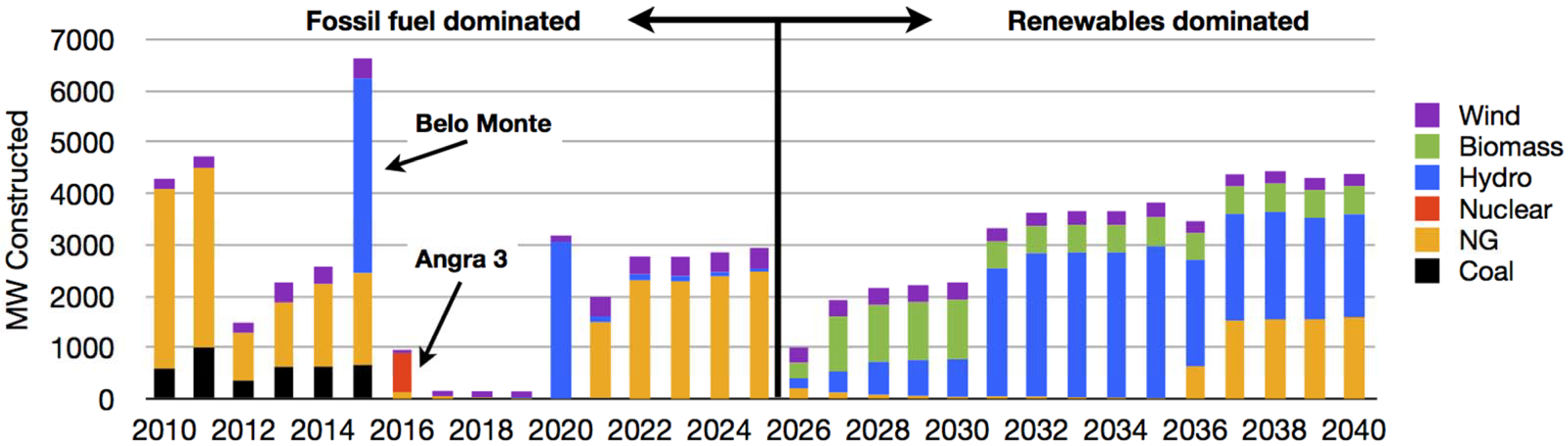
The initial output of the model is the expected per-source construction.
Figure 3 shows capacity additions for an average trial, divided into two distinct patterns. The first decade primarily expands natural gas, with some known construction of nuclear and hydro and a small expansion of coal-fired generating capacity. Natural gas is currently used as a peaking fuel to allow optimized hydropower generation. Going forward, an increasing amount of NG capacity is expected to be used for dedicated base load power. The small amount of additional coal capacity is a primary driver of GHG intensity—a problem discussed further in
Section 4. The hydropower capacity added during this time is from projects in progress such as Belo Monte. The known projects provide enough supply that little extra capacity is required from 2016 to 2020, resulting in a decrease before another round of NG additions. Small amounts of wind are added throughout the entire scenario as the demand increases continually on both an absolute and percentage basis.
Figure 3.
Capacity constructed by year under a representative case for the BAU scenario.
Figure 3.
Capacity constructed by year under a representative case for the BAU scenario.
The second half of the scenario shifts from adding NG to adding hydropower and more biomass capacity. It is expected that simple conversions of existing capacity will enable biomass generation up to 2025, but afterwards new capacity is required in our model. The hydropower capacity is expected to be built primarily in the Amazon, as high-quality dam sites outside of the tropical zones have mostly been utilized. The lower capacity factor of these tropical dams requires more capacity for the same amount of generation, along with a higher propensity for methane bubbling from annually flooded biomass. The higher per-MWh GHGs from these dams relative to southern temperate dams has the potential to double the fraction of GHGs from hydropower and increase the per-MWh intensity by a factor of four by 2040 when reservoir emissions are included. Dams are also responsible for the peaks in 2015 and 2031 seen in
Figure 4 under energy consumption. The two peaks correspond to initial construction of Angra 3 and Belo Monte during the mid-2010s, and a large addition to hydroelectric capacity in the 2030s. Long term increases in non-construction energy intensity are attributable to increased use of natural gas, which has the highest individual MJ/MWh intensity [
55]. Increased use of LNG would further increase energy consumption/MWh, a case not examined in this work.
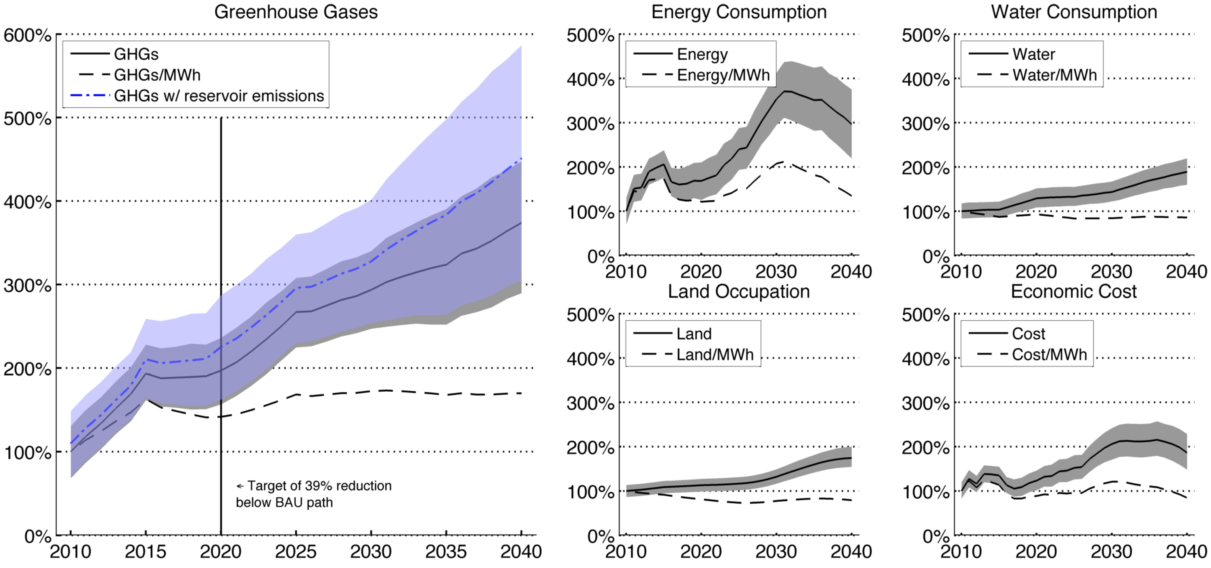
The final outputs of the model are the annual impacts, shown for all five impact categories (GHGs, energy, water, land, and cost) under the reference case (BAU) scenario in
Figure 4. Values are shown on both an absolute and per-MWh basis, normalized to the 2010 values from the first year of model results. With total electrical demand increasing by a factor of two, impacts in all categories rise on an absolute basis by 2040. The largest increases are in GHGs and energy, with slower rises in absolute water consumption, land occupation, and economic cost, and decreases in the per-MWh values of these later three impact categories.
GHGs are shown with emissions from hydroelectric reservoirs as additional impact, along with their large uncertainty. The midpoint shown including reservoir emissions assumes that 50% of gross emissions from reservoirs are natural, leaving 50% as net emissions, while the shaded region demonstrates net emissions from 10% to 90% of gross. This additional source of emissions represents a potentially large addition to existing impacts, but is associated with high uncertainty. The bulk of the emissions are from non-reservoir sources, with increases driven by fossil fuels, rising demand, and occasionally construction. With reservoir emissions included, there is the potential for later increases in GHGs to be driven by tropical hydropower.
Figure 4.
Annual results for the base case (BAU) scenario, for both absolute impacts and impact per unit energy. Results are normalized by respective values calculated for 2010, with shading denoting a 90% confidence interval. Energy consumption refers to primary energy without the energy included in fuels. The line and interval for GHGs including reservoir emissions shows net emissions as 10%, 50%, and 90% of gross emissions.
Water consumption and land use follow similar paths, driven by inertia from and changes to hydroelectric generation, particularly in the latter half of the time period studied. The impact factors for water consumption and land use are an order of magnitude higher for hydroelectricity than for other sources, and the existing dominance of hydropower dampens impacts shifts that result from the use of a more diverse generation mix. Both impact categories show a decrease in per-MWh impacts over the course of the scenario as a more diverse generation mix allows new generating capacity without significant increases in water consumption or new flooded land. The slightly larger increases in land occupation during the final decade are associated with the late build-out of Amazonian hydroelectricity, which will likely create larger reservoirs and associated increases in evaporation. Increased construction of tropical dams does not prohibit meeting 2020 deforestation reduction targets, but other forms of deforestation have less breathing room if targets are met.
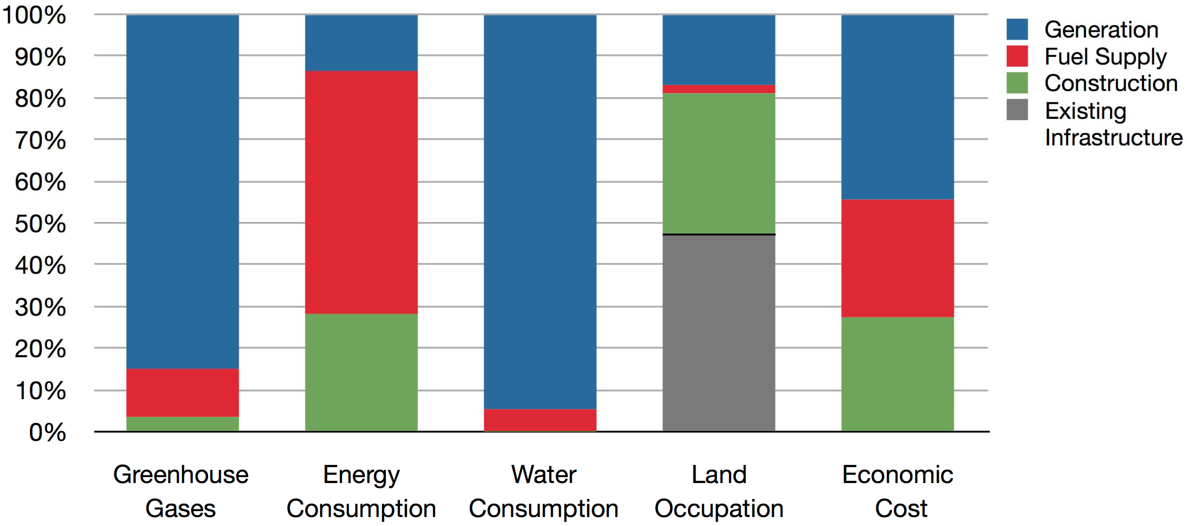
Energy consumption and cost are driven primarily by construction, which results in intermittent peaks throughout the course of the scenario. Much of this construction is again driven by hydropower, but alternative sources such as nuclear or solar power can also result in peaks due to expensive or intensive building requirements. From a cumulative perspective, these two impact categories, as well as the monotonic increase in land occupation, have a high fraction of impacts from construction, as seen in
Figure A1. This dependence is related to interest rates for initial capital, and the apparent decrease towards the end of the scenario represents the completion of a large build-out of tropical hydropower. The construction and associated impacts end because no future demands past 2040 are included to retroactively initiate advance construction, and a real-world continued expansion would likely not show these decreases in cost or energy consumption.
3.2. Climate Commitments
Total GHG emissions from electricity rise to 360% of its 2010 value by 2040. This rise is driven by several factors, as described above, and may make existing and potential carbon reduction commitments more difficult to meet, even though electricity is currently a small fraction of the country’s overall carbon footprint. Brazil has a national goal of reducing its national carbon footprint by 39% relative to a BAU pathway by 2020, and a target of reducing deforestation to 3925 km
2/year, down from historic rates of 1 × 10
4–2 × 10
4 km
2/year [
56,
57]. The BAU pathway, designated in 2007, is based on potential increases from 2005 emissions, and allows an increase of ~33% over actual 2010 emissions while still meeting the 39% reduction goal. This increase, from ~1500 Mt CO
2-eq to 2080 Mt CO
2-eq, will be dominated by increases in emissions from energy, industry, and agriculture, with additional space provided by continuing decreases in deforestation. With 2010 deforestation of 6450 km
2 [
57], meeting the 2020 deforestation target will result in a decrease of 39% in land cleared, and a 27% reduction in carbon emissions overall relative to 2010, assuming average per-acre impacts. This provides space for a 60% increase in emissions from sectors aside from deforestation.
The results of this work suggest, however, that increases in electricity-related emissions will increase by 104% from 2010 levels by 2020, without considering emissions from hydropower plants’ reservoirs. As electricity currently represents 6.7% of GHG emissions [
58], meeting the overall emissions target with this increase in electricity-related GHGs will require slower growth in emissions from other sectors such as transportation, industry or agriculture. The results suggest that meeting Brazil’s carbon targets may require additional effort beyond current plans [
59]. In addition, current estimates of carbon footprint do not take reservoir emissions into account because of the large inherent uncertainties [
60]. Resolving these uncertainties will require additional field work to gather more robust data from additional sites.
If reservoir impacts are included, electricity’s cumulative GHGs may increase by 3%–28% in our model (10%–90% of cumulative gross emissions). The rise in electricity-related GHGs is expected with national development and an associated increase in
per-capita energy use, but would make it more difficult to find sufficient reductions to meet stated greenhouse gas emissions targets. The continued rise in the second half of the scenario support a cautious view of the achievability of future carbon emissions targets by Brazil, particularly as deforestation declines as a percentage of emissions while energy and electricity increase. Identifying the best approaches to avoiding these issues is done using a decomposition approach in
Section 4.
3.3. Tradeoffs from Renewables
Brazil’s low GHG intensity for electricity has been enabled by use of its plentiful renewable resources, which have been assumed to have no to low emissions—both hydropower and biomass. The move towards increased use of natural gas and tropical hydroelectric dams will unavoidably increase GHG emissions. Recent evidence around tropical reservoir emissions continues to support this claim though, as discussed below, much more work is still needed [
7,
46].
Hydropower has provided Brazil with a large amount of energy and the ability to grow its economy, all with lower GHGs than the fossil fuels used to energize development in much of the rest of the world. These benefits have come at the cost of significant and often unmeasured ecosystem impacts. Water consumption is used as an ecosystem metric in this model, and is understandably high for hydropower, but evaporation is only a small piece of overall impacts. Land occupation helps to capture impacts to potential or existing communities, but is again a proxy for more complex impacts. Issues such as biodiversity, and species migration, or social impacts to surrounding communities lack comprehensive or widely accepted methods for measurement and incorporation into life-cycle studies. Further, though reservoirs are acknowledged as a net source of methane relative to the ecosystem present before the dam’s construction, the connection between gross and net emissions is unknown, and, along with land occupation, is likely to have significant variation from dam to dam. While tropical dams have the potential to flood more land per unit of capacity, environmental regulations make it unlikely that they will be built as such. The information used in this model is the best available but still represents less than 15 dams. The use of Monte Carlo methods incorporate this uncertainty, but better information is still necessary to refine estimates or include more direct impacts. The lack of information shows a need, particularly for Brazil, for increased measurements and work so that models such as this one can be more inclusive and inform better decisions about including hydropower and other sources as part of powering sustainable development. Particularly alarming in light of these higher impacts from tropical reservoirs and their role in our results is the inclusion of hydro projects in Clean Development Mechanism (CDM) projects aimed at reducing carbon emissions [
61]. The tradeoffs between GDP, GHGs, and ecosystems must be considered in light of sustainable development goals, balancing additional electricity off of ecosystem and community damage and likely increases, rather than savings, in GHGs.
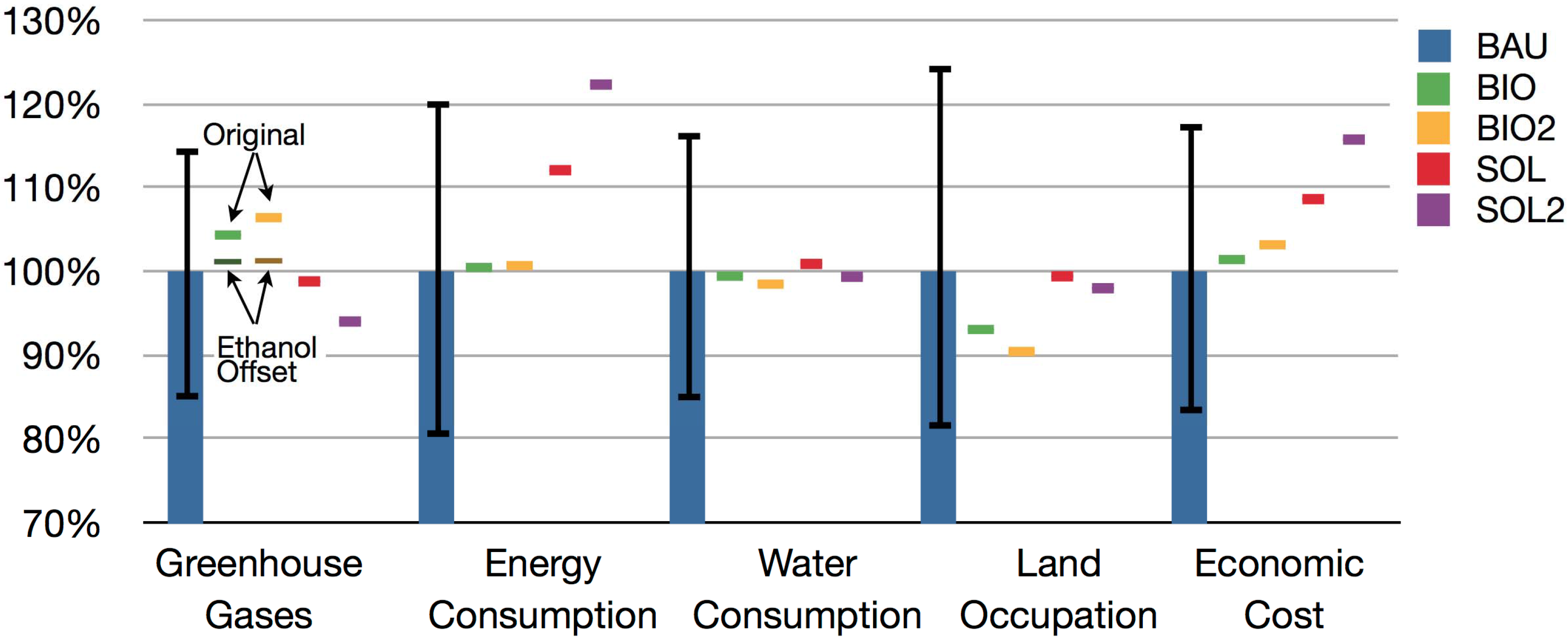
One proposed alternative to hydropower would be an expansion in solar power in addition to the wind power expected by the MESSAGE scenarios, or the production of additional ethanol from biomass via hydrolysis rather than producing electricity, possibly as a more effective utilization. These alternatives were explored via the side cases from the BAU case, and cumulative results can be found in
Figure A2. The results show limited change and more tradeoffs. Switching the use of biomass from electricity to additional ethanol has negligible changes to GHGs when the avoided emissions from oil are considered. The other categories show drops in land occupation and water consumption, similar energy consumption, and higher cost, none of which include offsets from ethanol. Although the savings from not producing oil may reduce the extra cost of the biomass side cases, processing biomass to hydrolysis will require more water and energy than combusting it for electricity, possibly outweighing any gains in those areas. In the solar cases, overall GHGs are reduced at the price of higher—but uncertain—energy consumption during construction, and likely higher costs. Some land savings occur, but the low energy density of solar minimizes savings over hydropower.
The side cases show that, regardless of the sources chosen, attempting to maintain a low per-MWh GHG intensity through the use of other renewables will incur impacts in other categories, and continuing to rely on hydropower may result in higher impacts in all categories. In many ways, even with high uncertainty, GHGs are one of the best studied impact categories. While our results show that scenarios and existing data can help examine impacts and future trends, these tools will remain incomplete until more data exists on net emissions from reservoirs, and some data exists for broader ecosystem impacts from all renewable sources. This information is necessary to guide good policy-making for more sustainable development.
4. Conclusions
Brazil has different power generation characteristics from most ‘developed’ countries because of the amount of hydropower and the use of on-site sugarcane bagasse. Brazil’s future development will require additional electricity, which is likely to come from a more diverse set of generation types. With the supply-side trajectory projected for this work, the results indicate that Brazil may have more difficulty meeting carbon targets because of increased electricity-related GHG emissions. Identifying ways to change GHG emissions requires factoring impacts into metrics such as
per-capita electricity use or impacts per unit electricity. Emissions intensity per MWh at the start of the BAU scenario is 159 kg CO
2-eq/MWh, significantly lower than the U.S. average of 748 kg CO
2-eq/MWh [
6].
Per-capita electrical demand is also much lower for Brazil than the U.S., at 2.4
vs. 14.2 MWh/
capita in 2010 [
5]. Going forward, the BAU scenario shows GHG emissions intensity growing by 47% by 2020 and 82% by 2040, with
per-capita electricity demand growing by 28% by 2020 and 89% by 2040, after adjusting for projected population growth [
62]. Other impact categories show smaller increases or decreases in intensity, but grow on an absolute basis because of increases in population and
per-capita consumption.
Maintaining a relatively low-carbon electricity supply requires efforts on both supply-side emissions intensity and
per-capita demand. In the short term, addressing emissions intensity suggests avoiding growth in coal-fired generation, as increases in the use of coal are a primary factor in the early rise in carbon intensity during the mid 2010s (
Figure 3 and
Figure 4). Avoiding additional infrastructure and use of coal while it remains a small portion of the generation mix prevents future challenges in shifting away from coal. Over longer time scales, avoiding natural gas through increased hydroelectric generation may enable emissions intensity to remain low—though there is large uncertainty in this area—at the cost of increased water and land related impacts, as well as increasing public protest. Avoiding natural gas in general may be difficult due to a lack of easily scaled generation options—there is a finite supply of bagasse, and nuclear plants likely cannot be constructed in time to meet 2020 goals, though they may be an expensive option for longer-term objectives. Solar and wind remain as possibilities for reducing emissions intensities, though they will incur larger capital costs than NG and are similarly low-density in land occupation as hydropower. Brazil’s efforts to expand wind are ongoing and may be key to maintaining low GHG emissions intensity.
In addition to supply-side policies and changes, reductions in demand—beyond the MAED model predictions that this work is based on—may be sensible. Without compromising quality of life, there are likely efficiencies that can be implemented in industrial processes, as identified by the World Bank [
19]. If these efficiencies are insufficient and climate change goals hold enough significance, reductions in
per-capita demand through conservation would be required. Because of variations in development between major cities and some rural areas, conservation in some regions could allow others to continue increasing consumption while still reducing
per-capita electricity consumption for the country as a whole. Combinations of supply- and demand-side approaches, based on perceived feasibility, can easily be tested using the model presented in this work.
Hydropower plays a central role in Brazilian electricity, but the impacts of future dams are very uncertain. Data on ecosystem impacts beyond GHGs is sparse, and uncertainty about net GHG emissions and land usage from tropical hydroelectric reservoirs may reduce viability of expanding hydroelectricity. Hydropower in Brazil is an excellent example of model outputs as well as the absence of data informing a need for future work. Of particular concern is the ratio between net and gross emissions, and the long-term trends in reservoir emissions. Additional measurements are needed around seasonal and multi-year emission measurements, as well as assessments of sites before and after dams are built to estimate net emissions. While all major emissions mechanisms—bubbling, degassing, and diffusion—would benefit from improved data and a wider array of test sites, tracking methane emissions and anaerobic decomposition of biomass are of particular interest due to methane’s high GWP. Efforts to reduce Brazil’s GHG emissions should start by assessing the current impacts of its largest electricity source.
The underlying model in this work allows the examination of life-cycle impacts, major impact drivers, and infrastructure construction on an annual basis, rather than at scenario endpoints. While the annual resolution offers additional clarity to planners, future work could match this model with one that uses time slices to include daily or seasonal variations in electrical supply and demand for a more detailed feasibility assessment.
The presented results discuss electricity for a single region, with a focus on GHG emissions, but the model has the potential to assess broader questions in other regions. Future work could expand upon this model, adding data and calculations for energy use in transport and heating, as well as impacts from water and wastewater treatment. These additional classes of demand can allow the examination of questions about the use of new energy sources such as shale gas, interconnections between energy and water supplies, or the lowest-impact options for shifting away from non-renewable sources. With an increasing set of jurisdictions around the world investigating the environmental impacts stemming from energy supplies, quantitative tools such as this model can play a critical role in understanding and developing policies and scenarios to meet both environmental and economic goals.


